Inside–Out Method for Simulating a Reactive Distillation Process

1
Institute for Process System Engineering, Qingdao University of Science and Technology, Qingdao 266042, China
2
Petro-Cyber Works Information Technology Company Limited Shanghai Branch, Shanghai 200120, China
*
Author to whom correspondence should be addressed.
Processes 2020, 8(5), 604; https://doi.org/10.3390/pr8050604
Submission received: 30 March 2020
/
Revised: 11 May 2020
/
Accepted: 13 May 2020
/
Published: 19 May 2020
(This article belongs to the Special Issue Chemical Process Design, Simulation and Optimization)
Abstract
:Reactive distillation is a technical procedure that promotes material strengthening and its simulation plays an important role in the design, research, and optimization of reactive distillation. The solution to the equilibrium mathematical model of the reactive distillation process involves the calculation of a set of nonlinear equations. In view of the mutual influence between reaction and distillation, the nonlinear enhancement of the mathematical model and the iterative calculation process are prone to fluctuations. In this study, an improved Inside–Out method was proposed to solve the reaction distillation process. The improved Inside–Out methods mainly involved—(1) the derivation of a new calculation method for the K value of the approximate thermodynamic model from the molar fraction summation equation and simplifying the calculation process of the K value, as a result; and (2) proposal for an initial value estimation method suitable for the reactive distillation process. The algorithm was divided into two loop iterations—the outer loop updated the relevant parameters and the inside loop solved the equations, by taking the isopropyl acetate reactive distillation column as an example for verifying the improved algorithm. The simulation results presented a great agreement with the reference, and only the relative deviation of the reboiler heat duty reached 2.57%. The results showed that the calculation results were accurate and reliable, and the convergence process was more stable.
1. Introduction
Reactive distillation combines the chemical reaction and distillation separation process in a single unit operation [1]. As reactive distillation has the advantages of improving reaction conversion rate and selectivity and reducing costs, the research on design and optimization of the reactive distillation processes has increased rapidly in recent years [2]. Now reactive distillation technology has been successfully applied to the areas of esterification, etherification, hydrogenation, hydrolysis, isomerization, and saponification [3].
The production of methyl tert-butyl ether (MTBE), methyl tert-pentyl ether (TAME), and ethyl tert-butyl ether (ETBE), etc., adopts the reactive distillation technology, and the reaction conversion rate was significantly higher than the fixed-bed reactors [4]. Using the reactive distillation technology to produce methyl acetate can reduce investment and energy costs to one-fifth, and the reaction conversion rate is close to 100% [5]. Zhang et al. proposed a novel reaction and extractive distillation (RED) process and used it for the synthesis of isopropyl acetate (IPAc). The results showed that the purity of IPAc reached 99.5% [6].
As distillation and reaction take place simultaneously, there are complex interaction effects between them [7]. Therefore, it is very important to use mathematical methods to model and simulate the reactive distillation process, and optimize the operating conditions and equipment parameters [8]. The traditional algorithms for simulating reactive distillation include the tridiagonal matrix method, the relaxation method, the simultaneous correction method (Newton–Raphson), and the homotopy method.
Zhang et al. proposed a mathematical model of the heterogeneous catalytic distillation process. For the boundary value problem solved by the model, the multi-target shooting method and the Newton–Raphson iteration were used. The calculation results were consistent with the experimental data [9]. The partial Newton method proposed by Zhou et al. used the results from a repeated relaxation method as the initial value of the iteration variable, and then used the Newton–Raphson method to solve the MESHR equation (material balance, phase equilibrium, molar fraction summation, enthalpy balance, chemical reaction rate) [10]. Qi et al. aimed at the equilibrium reactive distillation process and transformed the physical variables such as the stage composition, flow, and enthalpy, such that the transformed mathematical model of the reactive distillation was completely consistent with the ordinary distillation and the modified Newton–Raphson method was used to solve it [11]. Juha introduced the homotopy parameters in the phase equilibrium, the enthalpy equilibrium, and the chemical reaction equilibrium equations, to establish a homotopy model of reactive distillation, and successfully simulated an MTBE reactive distillation column [12]. Wang et al. used the relaxation method to calculate the methyl formate hydrolysis catalytic distillation column. The simulation results were compared with the experimental ones and showed great agreement [13]. Steffen and Silva divided the reactive distillation model into several smaller sets of equations based on the equation tearing method, and obtained a set of linear and nonlinear equations each, which simulated chemical reactions [14].
Boston and Sullivan first proposed the Inside–Out method to simulate a multi-component ordinary distillation process [15,16]. Compared to other algorithms, two thermodynamic property models are used. The approximate thermodynamic models are used for frequent inside loop calculations to solve the MESH equation (material balance, phase equilibrium, molar fraction summation, enthalpy balance). The strict thermodynamic models are used for outer loop calculations of the phase equilibrium constant K and the approximate model parameters. This saves a lot of time when calculating thermodynamic properties. The inside loop uses a stripping factor (Sb) as an iterative variable, which integrates the effects of the stage temperature and the vapor and liquid flow rates, reduces the number of iterative variables, and improves the stability of convergence.
Russell further improved the Inside–Out method by solving the sparse tridiagonal matrix and applying the improved Thomas Chase method, and applied it to the calculation of crude oil distillation [17]. The modified Inside–Out method was proposed by Saeger, who added a two-parameter model for liquid composition, representing the effect on phase equilibrium constant, improving the convergence stability of highly non-ideal systems, and improving the convergence rate [18]. Jelinek simplified the Inside–Out method proposed by Russell; the simplified method could solve the distillation process specified by any operation and did not use an approximate enthalpy model in the inside loop, reducing the complexity of the calculation process [19].
Basing the Inside–Out method on simulating ordinary distillation process, increased the chemical reaction rate equation and established a mathematical model of the reactivedistillation. In view of the obvious enhancement of the nonlinearity of the mathematical model, it was more difficult to solve the problem than ordinary distillation [20]. This study used the Inside–Out method to solve the reactive distillation process, simplified the calculation of the K value of the approximate thermodynamic model, and proposed an initial value estimation method. This is an in-house model.
2. Mathematical Model
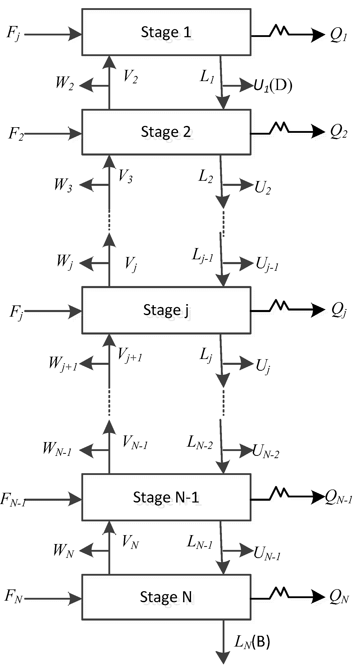
The schematic diagram of the reaction distillation column is shown in Figure 1. The whole column is composed of N stages. The condenser is regarded as the first stage and the reboiler is regarded as the last stage. There can be a liquid phase product, a vapor phase product, and a free water product at the top of the tower, and a liquid phase product at the bottom of the column. Chemical reactions can take place anywhere in the column. The general model of the jth theoretical stage is shown in Figure 2, where Fj is the feed flow rate of stage j, Lj is the liquid flow rate outputting stage j, and inputting stage j + 1, Vj is the vapor flow rate outputting stage j and inputting stage j − 1, Uj is the liquid side flow rate outputting stage j, Wj is the vapor side flow rate outputting stage j, Qj is the heat duty from stage j, Rr,j is the reaction extent of the rth reaction on stage j. The schematic representation from Figure 2 to represent all stages are shown in Figure 3.
The stages of the column are assumed to be in equilibrium conditions, the vapour and liquid phases leaving the stage are assumed to be in thermodynamic equilibrium, the stage pressure, temperature, flow, and composition are assumed to be constant at each stage. Five sets of equations are used to describe the equilibrium state of the stage—the material balances, the phase equilibrium, the molar fraction summation, the enthalpy balance, and the chemical equilibrium equations.
A set of highly nonlinear equations was obtained by modeling the steady state process of the reactive distillation column. The non-linearities were in the phase equilibrium, enthalpy balances, and chemical equilibrium equations. The solution of model equations is very difficult and the convergence depends strongly on the goodness of the initial guesses. After choosing appropriate iterative variables and providing the initial value of variables, the iterative calculation process can start. When the iterative calculation converges, the stage temperature, flow, and composition profiles can be obtained.
The mathematical model of reactive distillation [21]:
(1) Material balance Equation (M):
(2) Phase equilibrium Equation (E):
(3) Molar fraction summation Equation (S):
(4) Enthalpy balance Equation (H):
(5) Chemical reaction rate Equation (R):
3. Algorithm
3.1. Inside–Out Method
The Inside–Out method divides the mathematical model into an inside and outer loop for iterative calculation, and uses two sets of thermodynamic models, a strict thermodynamic model and an approximate thermodynamic model (K value model and enthalpy value model). The simple approximate thermodynamic model was used for frequent inside loop calculations to reduce the time it takes to calculate the thermodynamic properties. The strict thermodynamic model was used for the outer loop calculations, and the parameters of the approximate thermodynamic model were corrected at the outer loop.
Defining the inside loop variables—relative volatility αi,j, stripping factors Sb,j of the reference components, liquid phase stripping factors RL,j, and the vapor phase stripping factors RV,j.
The inside loop uses the vapor and liquid phase flow rates of each component instead of the composition, for the calculations. Their relationship with the vapor and liquid phase composition and flow is as follows:
According to the inside loop variables defined by the mathematical model of the Inside–Out method, the material balance Equation (M) and the phase equilibrium Equation (E) can be rewritten into the following relationship.
Material Balance:
Phase balance:
3.1.1. Strict Thermodynamic Model
The strict model is mainly used for the outer loop to correct the parameters in the approximate thermodynamic model, including the calculation of the phase equilibrium constant K value, and the vapor-liquid enthalpy difference, as follows:
3.1.2. Approximate Thermodynamic Model
① K-value model
Define a new variable for the K value of the reference component, Kb,j, and the reference component b is an imaginary component. Kb,j was calculated by the following formula, where ωi,j is a weighting factor.
The relationship between Kb,j and the stage temperature Tj is related using Equation (17), T* is the reference temperature.
The value of the parameter Bj can be obtained by the differential calculation of 1/T by the Kb, and the temperatures Tj−1 and Tj+1 of the two adjacent stages are selected as T1 and T2.
② Enthalpy model
The calculation of the enthalpy difference is the main time-consuming part of the entire enthalpy calculation, so the calculation of the enthalpy difference was simplified in the approximate enthalpy model, and a simple linear function was used to fit the calculation of the enthalpy difference.
3.1.3. Improved K-Value Model
The K-value model was improved by simplifying the calculation of the weighting factor. This was derived from the molar fraction summation equation. The derivation process is shown below.
The relationship between the K value of the reference component Kb,j and the K value of the common component is:
The weighting factors need to satisfy:
The stage temperature needs to satisfy the following relationship:
The introduction of new variables ui,j was defined as:
The new relationship is:
Since Kb,j was calculated by Ki,j through a weighting function, the trend with temperature changes was the same, so uj,i is a temperature-independent parameter, so at the stage temperature:
The derivative of and at the stage temperature was equal to:
The weighting function used the new calculation method:
3.2. Initial Value Estimation Method
The system of equations obtained from the modeling of the steady-state reactive distillation process was non-linear and was very difficult to solve. Therefore, it was important to provide good initial estimates, otherwise it would not be possible to reach a solution.
Before providing good initial estimates, all feed streams were mixed to perform chemical reaction equilibrium calculations to obtain a new set of compositions and flow rate, which were used to calculate the initial value of the variable.
Temperature: Calculate the dew and bubble point temperature by flash calculation, which was used as the initial temperature at the top and at the bottom of the tower. The initial temperature of the middle stages was obtained by linear interpolation.
Composition: The composition calculated by isothermal flash calculation was used as the initial value of the vapor-liquid composition of each stage.
Flow: According to the constant molar flow rate assumption and the total material balance calculation, the initial value of the vapor–liquid flow rate of each stage was obtained
Reaction extent: The reaction extent calculated by the chemical reaction equilibrium was taken as the maximum value of the reaction extent in the reaction section. According to the feeding condition of the reaction section, the position with the maximum reaction extent was selected. If there was only one feed in the reaction section, the position of the feed stage was selected. If there were multiple feeds in the reaction section, the position of the feed stage near the reboiler was chosen. If there was no feed in the reaction section, the position of the reaction stage closest to the feed was selected. The initial value of the reaction extent of the other stages were calculated according to the maximum value and a certain proportion of attenuation. The calculation is shown below.
Between the first reaction stage and the stage with the maximum reaction extent:
Between the stage with the maximum reaction extent and the last reaction stage:
where Rmax is the maximum value of the reaction extent in the reaction section, jm is the stage position where the maximum reaction extent occurs; j1 is the first stage position in the reaction section; and jn is the last stage position in the reaction section.
3.3. Calculation Steps and Block Diagram
The reactive distillation column adopts an improved Inside–Out method for calculation. The main working idea is that the the outer loop used a strict thermodynamic model to calculate the phase equilibrium constant and the vapor–liquid phase enthalpy difference, and the results were used to correct the approximate thermodynamic model parameters and update the reaction extents of each stage. The inside loop uses an approximate thermodynamic model to solve the MESHR equation to obtain the stage temperature, flow rate, and composition. After the inside loop calculation converges or reaches the number of iterations, the model returns to the outer loop to continue the calculation. When the inside and outer loop converges at the same time, the calculation ends.
The calculation steps are shown below:
1. Given initial value
(1) According to the feed, pressure, and operation specifications, the initial values of the temperature, flow rate, composition, and the reaction extent are provided (Section 3.2).
2. Outer loop iteration
(2) Calculate the phase equilibrium constant Ki,j with a strict thermodynamic model, and then calculate parameters Kb,j, A, and B in the K-value model.
(3) Calculate the vapor–liquid phase enthalpy difference using a strict thermodynamic model, and fit the parameters cj, dj, ej, and fj in the approximate enthalpy model.
(4) Calculate the stripping factors Sb,j, relative volatility αi,j, liquid phase stripping factors RL,j, and vapor phase stripping factors RV,j.
(5) Calculate the reaction extent according to the reaction conditions. The chemical reaction can be a specified conversion rate or a kinetic reaction, and the kinetic reaction rate is calculated by a power law expression.
Power law expression:
T0 is not specified:
T0 is specified:
(6) Outer convergence judgment conditions:
3. Inside loop iteration
(7) According to the material balance Equation (13), a tridiagonal matrix was constructed, and then the liquid flow rate li,j of each component was obtained by solving the matrix. Using the phase equilibrium Equation (14), the vapor phase flow rate vi,j of each component was obtained.
(8) The vapor–liquid flow rates Vj and Lj can be calculated by Equation (9), the vapor–liquid phase composition xi,j and yi,j can be calculated by Equation (8).
(9) Combining the bubble point equation with Equation (9) to obtain Equation (39), a new set of K values Kb,j of the reference components can be calculated.
According to Equation (40), a new set of stage temperature can be calculated using the new Kb,j values.
Now, the correction values of the vapor–liquid flow rate, composition, and temperature are obtained. They satisfy the material balance and phase equilibrium equation, but does not satisfy the enthalpy equilibrium equation. In the following, the iterative variable of the inside loop should be modified according to the deviation of the enthalpy balance Equation (10). Select lnSb,j as the inside loop iteration variable. If there are side products, the side stripping factors lnRL,j and lnRV,j should be added as the inside loop iteration variables. Taking the enthalpy balance equation as the objective function, the enthalpy balance equation of the first and last stage should be deleted and replaced with two operation equations of the reactive distillation column.
(11) Calculate the vapor–liquid phase enthalpy according to the simplified enthalpy model.
(12) Calculate the partial derivative of the objective function to the iterative variable and construct the Jacobian matrix. The Schubert method was used to calculate the modified value of the inside iteration variable [22,23]. Damping factors can be used if necessary.
(13) Using the new inside iteration variable value, repeat steps (7) to (9) to obtain the new stage flow, composition, and temperature, and calculate the error of the objective function. If the error was less than the convergence accuracy of the inside loop, return to the outer loop to continue the calculation, otherwise repeat the calculation from Step (11) to Step (13). The calculation block diagram of the improved Inside–Out method is shown in Figure 4.
4. Results
4.1. Example 1: Isopropyl Acetate
Taking the process of synthesizing isopropyl acetate (IPAc) with acetic acid (HAc) and isopropanol (IPOH) as an example, the esterification reaction is a reversible exothermic reaction, and the conversion rate is limited by the chemical equilibrium. Zhang et al. proposed reactive and extractive distillation technology for the synthesis of IPAc, and the extraction agent dimethyl sulfoxide (DMSO) was added in the tower to obtain high-purity IPAc [6]. Zhang et al. conducted a steady-state simulation of the reactive distillation column, and performed dynamic optimization control, based on the results. In this work, the improved Inside–Out method was used to solve the esterification process, and the steady-state simulation results were compared with that of Zhang et al. [6]. The chemical reaction equation of this esterification reaction was as follows:
Kong et al. determined the kinetic model of the esterification reaction through kinetic experiments [24]. The kinetic expressions and parameters are as follows:
where r is the reaction rate, mol·L−1·min−1; Ci is the molar volume concentration of the i component, mol·L−1; k+, and k– are the forward and reverse reaction rate constants; R is the gas constant, with avalue of 8.314 J·mol−1·K−1; and T is the temperature, in K.
The improved Inside–Out method was used to simulate the isopropyl acetate process. The property method was non-random two liquid (NRTL). The operating conditions of the isopropyl acetate reactive distillation column is shown in Table 1.
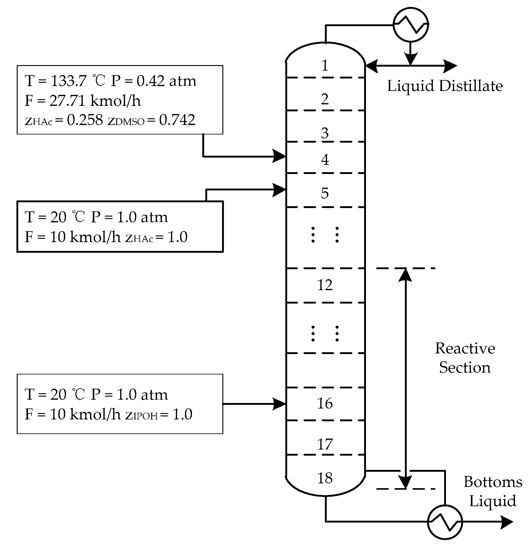
The schematic diagram of the isopropyl acetate reactive distillation column and the parameters of the feed stream are shown in Figure 5.
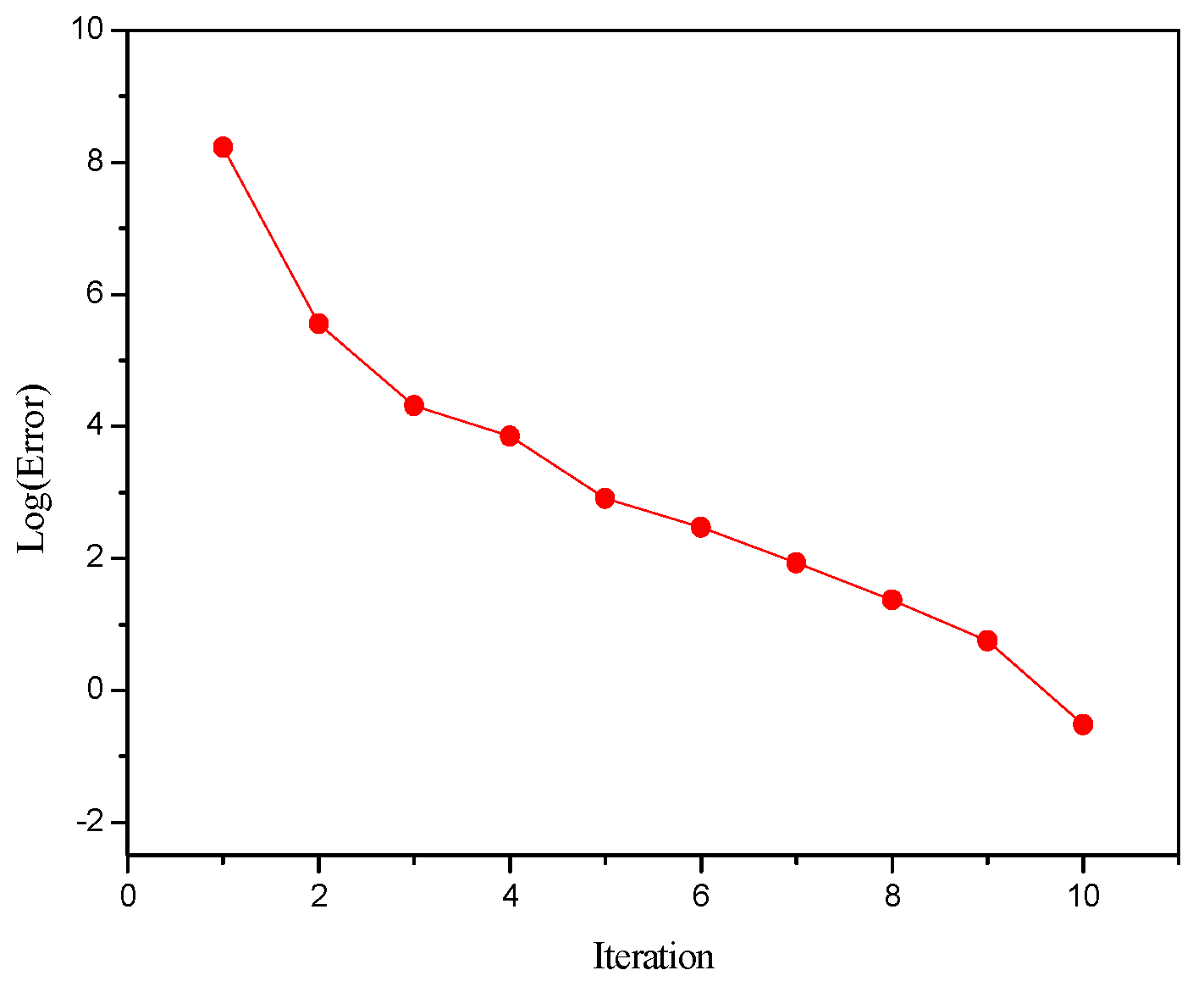
Figure 6 is a comparison between the initial value of the reaction extent and the simulation result. It can be seen that the initial value and the simulation results were relatively close, which increased the possibility of convergence. The error behavior at each iteration, calculated by Equation (38), for the program using the improved Inside–Out method is shown in Figure 7. The outer loop calculation reached the convergence through 10 iterations, and the error decreased steadily, without oscillation.
Table 2 shows the comparison between the simulation results of the isopropyl acetate reactive distillation column and the literature. It can be seen that the temperatures at the top and bottom of tower obtained in this work were similar to that in the literature, and the relative deviation was within 1%. The relative deviation of the condenser heat duty was 1.82% and the relative deviation of the reboiler heat duty was 2.47%.
Table 3 shows the comparison between the simulation results of the molar composition of the top and bottom products and the literature. It can be seen that the molar composition of the top and bottom product obtained in this work presented a great agreement with the literature, except for the smaller part, and the simulation results were accurate and reliable.
4.2. Example 2: Propadiene Hydrogenation
Taking the depropanization column in the propylene recovery system of the ethylene production process as an example. The Inside–Out method was used to simulate the depropanizer column, and the results were compared with the measured values. The top of the depropanizer column was equipped with a catalyst. In the reaction section, propadiene was hydrogenated into propylene and propane. The conversion rate of the first reaction was 0.485, the conversion rate of the second reaction was 0.015. The chemical reaction equation were as follows:
The improved Inside–Out method was used to simulate the depropanization column. The property method was Soave–Redlich–Kwong (SRK). The depropanizer column had 3 feeds, and the feed stream parameters are shown in Table 4. The operating conditions of the depropanization column are shown in Table 5.
Table 6 shows the comparison between the simulation results of the depropanization column and the measured value. It can be seen that the temperatures in the top and bottom products, as calculated by the Inside–Out method were close to the measured value, and the relative error was about 1%. The liquid product flow rate at the top and bottom of the tower coincided with the measured value, only the relative deviation of the vapor product flow at the top of the tower was 2.74%. Table 7 shows the comparison between the mass composition of the top and bottom liquid products and the measured value. The simulation results of the product mass compositions were basically consistent with the measured value, except for the smaller composition values.
5. Conclusions
Based on the process principle of reactive distillation, a mathematical model of reactive distillation process was established. The improved Inside–Out method was provided in this work for the solution of a reactive distillation process. In view of the nonlinear enhancement of the reactive distillation mathematical model and the difficulty of convergence, the calculation of the K value of the approximate thermodynamic model was improved to simplify the calculation process. The initial value estimation method suitable for the calculation of reactive distillation was proposed, which increased the possibility of convergence.
The algorithm was verified by using an isopropyl acetate reactive distillation column and a depropanization column as examples. In Example 1, the reaction extent calculated by the initial value estimation method was close to the simulation results, it facilitated the convergence process of the solution algorithm. The simulation results obtained in this work were compared with Zhang et al. [6], presenting great agreement with the reference, only the relative deviation of the reboiler heat duty reached 2.57%. In Example 2, the simulation results of the depropanization column presented a good agreement with the measured value, except for the smaller composition value. The results showed that the improved Inside–Out method calculation results were accurate and reliable.
Author Contributions
Conceptualization, X.S.; Data curation, J.W.; Formal analysis, S.X.; Project administration, L.X.; Writing—original draft, L.W.;Writing—review & editing, L.W. All authors have read and agreed to the published version of the manuscript.
Funding
This research was funded by Major Science and Technology Innovation Projects in Shandong Province, grant number [2018CXGC1102]; and The APC was funded by the Science and Technology Department of Shandong Province.
Conflicts of Interest
The authors declare no conflict of interest.
Abbreviations
| A:B | Parameters of the Approximate K-Value Model |
| C | Molar volume concentration |
| c,d,e,f | Parameters of the approximate enthalpy model |
| DMSO | Dimethyl sulfoxide |
| ETBE | Ethyl tert-butyl ether |
| E | Activation energy, J·mol−1 |
| F | Feed flow, mol·s−1 |
| vapor phase enthalpy, J·mol−1 | |
| Liquid phase enthalpy, J·mol−1 | |
| Vapor phase enthalpy difference,J·mol−1 | |
| Liquid phase enthalpy difference, J·mol−1 | |
| HAc | Acetic acid |
| IPAc | Isopropyl acetate |
| IPOH | Isopropanol |
| k+ | Forward reaction rate constants |
| k- | Reverse reaction rate constants |
| Phase equilibrium constant | |
| Phase equilibrium constant of reference component b | |
| Liquid flow, mol·s−1 | |
| MESH | Material balance, Phase equilibrium, Molar fraction summation, enthalpy balance |
| MESHR | Material balance, Phase equilibrium, Molar fraction summation, enthalpy balance, Chemical reaction rate |
| MTBE | Methyl tert-butyl ether |
| N | The number of distillation stages |
| NRTL | Non-random two liquid |
| Reaction extents, mol·s−1 | |
| Liquid stripping factor | |
| Vapor stripping factor | |
| r | Reaction rate |
| Stripping factor for reference component b | |
| T | Temperature, K |
| T* | Reference temperature, K |
| TAME | Methyl tert-pentyl ether |
| Liquid side product flow, mol·s−1 | |
| Vapor flow, mol·s−1 | |
| Vapor side product flow, mol·s−1 | |
| Liquid mole fraction | |
| Vapor mole fraction | |
| Feed mole fraction | |
| Stoichiometric coefficient | |
| Liquid holdup, m3 | |
| Relative volatility | |
| Tolerance | |
| Weighting factor | |
| i | Component i |
| j | Stage j |
References
- Gao, X.; Zhao, Y.; Li, H.; Li, X.G. Review of basic and application investigation of reactive distillation technology for process intensification. CIESC J. 2018, 69, 218–238. [Google Scholar]
- Li, C.L.; Duan, C.; Fang, J.; Li, H. Process intensification and energy saving of reactive distillation for production of ester compounds. Chin. J. Chem. Eng. 2019, 27, 1307–1323. [Google Scholar] [CrossRef]
- Ling, X.M.; Zheng, W.Y.; Wang, X.D.; Qiu, T. Advances in technology of reactive dividing wall column. Chem. Ind. Eng. Prog. 2017, 36, 2776–2786. [Google Scholar]
- Ma, J.H.; Liu, J.Q.; Li, J.T.; Peng, F. The progress in reactive distillation technology. Chem. React. Eng. Technol. 2003, 19, 1–8. [Google Scholar]
- Steffen, V.; Silva, E.A. Numerical methods and initial estimates for the simulation of steady-state reactive distillation columns with an algorithm based on tearing equations methodology. Therm. Sci. Eng. Prog. 2018, 6, 1–13. [Google Scholar] [CrossRef]
- Zhang, Q.; Yan, S.; Li, H.Y.; Xu, P. Optimization and control of a reactive and extractive distillation process for the synthesis of isopropyl acetate. Chem. Eng. Commun. 2019, 206, 559–571. [Google Scholar] [CrossRef]
- Tao, X.H.; Yang, B.L.; Hua, B. Analysis for fields synergy in the reactive distillation process. J. Chem. Eng. Chin. Univ. 2003, 17, 389–394. [Google Scholar]
- Lee, J.H.; Dudukovic, M.P. A Comparison of the Equilibrium and Nonequilibrium Models for a Multi-Component Reactive Distillation Column. Comput. Chem. Eng. 1998, 23, 159–172. [Google Scholar] [CrossRef]
- Zhang, R.S.; Han, Y.U. Hoffmann. Simulation procedure for distillation with heterogeneous catalytic reaction. CIESC J. 1989, 40, 693–703. [Google Scholar]
- Zhou, C.G.; Zheng, S.Q. Simulating reactive-distillation processes with partially newton method. Chem. Eng. (China) 1994, 3, 30–36. [Google Scholar]
- Qi, Z.W.; Sun, H.J.; Shi, J.M.; Zhang, R.; Yu, Z. Simulation of distillation process with chemical reactions. CIESC J. 1999, 50, 563–567. [Google Scholar]
- Juha, T.; Veikko, J.P. A robust method for predicting state profiles in a reactive distillation. Comput. Chem. Eng. 2000, 24, 81–88. [Google Scholar]
- Wang, C.X. Study on hydrolysis of methyl formate into formic acid in a catalytic distillation column. J. Chem. Eng. Chin. Univ. 2006, 20, 898–903. [Google Scholar]
- Steffen, V.; Silva, E.A. Steady-state modeling of reactive distillation columns. Acta Sci. Technol. 2012, 34, 61–69. [Google Scholar] [CrossRef]
- Boston, J.F.; Sullivan, S.L. A new class of solution methods for multicomponent multistage separation processes. Can. J. Chem. Eng. 1974, 52, 52–63. [Google Scholar] [CrossRef]
- Boston, J.F. Inside-out algorithms for multicomponent separation process calculations. ACS Symp. Ser. 1980, 9, 135–151. [Google Scholar]
- Russell, R.A. A flexible and reliable method solves single-tower and crude-distillation-column problems. Chem. Eng. J. 1983, 90, 53–59. [Google Scholar]
- Saeger, R.B.; Bishnoi, P.R. A modified “Inside-Out” algorithm for simulation of multistage multicomponent separation process using the UNIFAC group-contribution method. Can. J. Chem. Eng. 1986, 64, 759–767. [Google Scholar] [CrossRef]
- Jelinek, J. The calculation of multistage equilibrium separation problems with various specifications. Comput. Chem. Eng. 1988, 12, 195–198. [Google Scholar] [CrossRef]
- Lei, Z.; Lu, S.; Yang, B.; Wang, H.; Wu, J. Multiple steady states analysis of reactive distillation process by excess-entropy production (I) Establishment of stability model on steady state. J. Chem. Eng. Chin. Univ. 2008, 22, 563–568. [Google Scholar]
- Fang, Y.J.; Liu, D.J. A reactive distillation process for an azeotropic reaction system: Transesterification of ethylene carbonate with methanol. Chem. Eng. Commun. 2007, 194, 1608–1622. [Google Scholar] [CrossRef]
- Schubert, L.K. Modification of a quasi-Newton method for nonlinear equations with a sparse Jacobian. Math. Comput. 1970, 24, 27–30. [Google Scholar] [CrossRef]
- Liu, S.P. Compact Representation of Schubert Update. Commun. Appl. Math. Comput. 2001, 1, 51–58. [Google Scholar]
- Kong, S. The New Technology of Isopropyl Acetate Using Catalytic Distillation; Yantai University: Yantai, China, 2014; pp. 39–42. [Google Scholar]
Figure 1.
Schematic representation of the reactive distillation column.
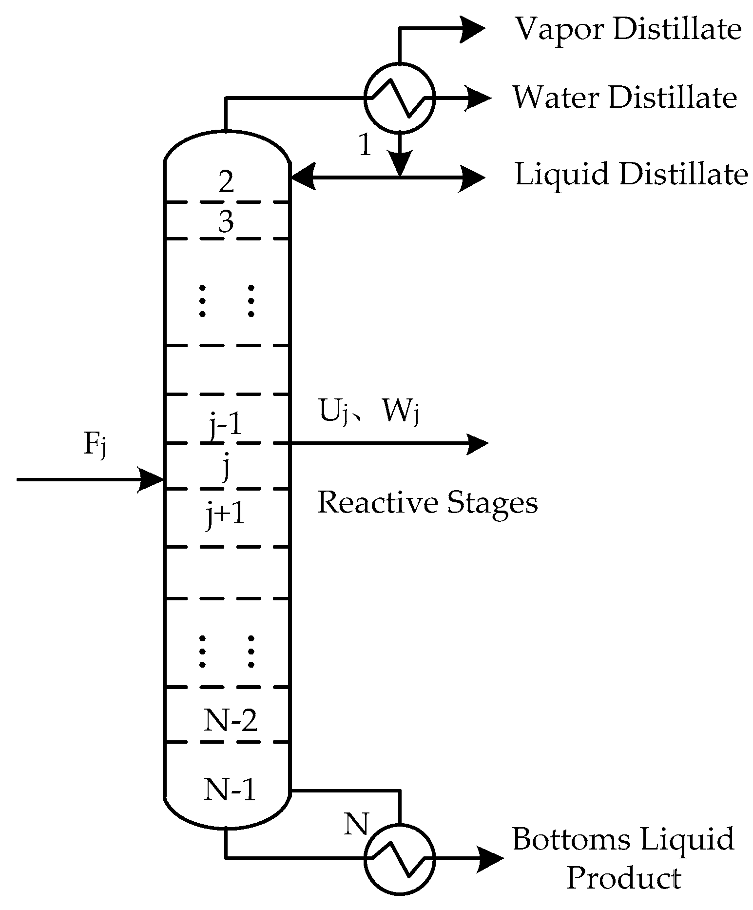
Figure 2.
The jth equilibrium stage of the reactive distillation column.

Figure 3.
Schematic representation of input and output streams in all stages of a distillation column.
Figure 3.
Schematic representation of input and output streams in all stages of a distillation column.

Figure 4.
Calculation of the block diagram of the improved Inside–Out method.
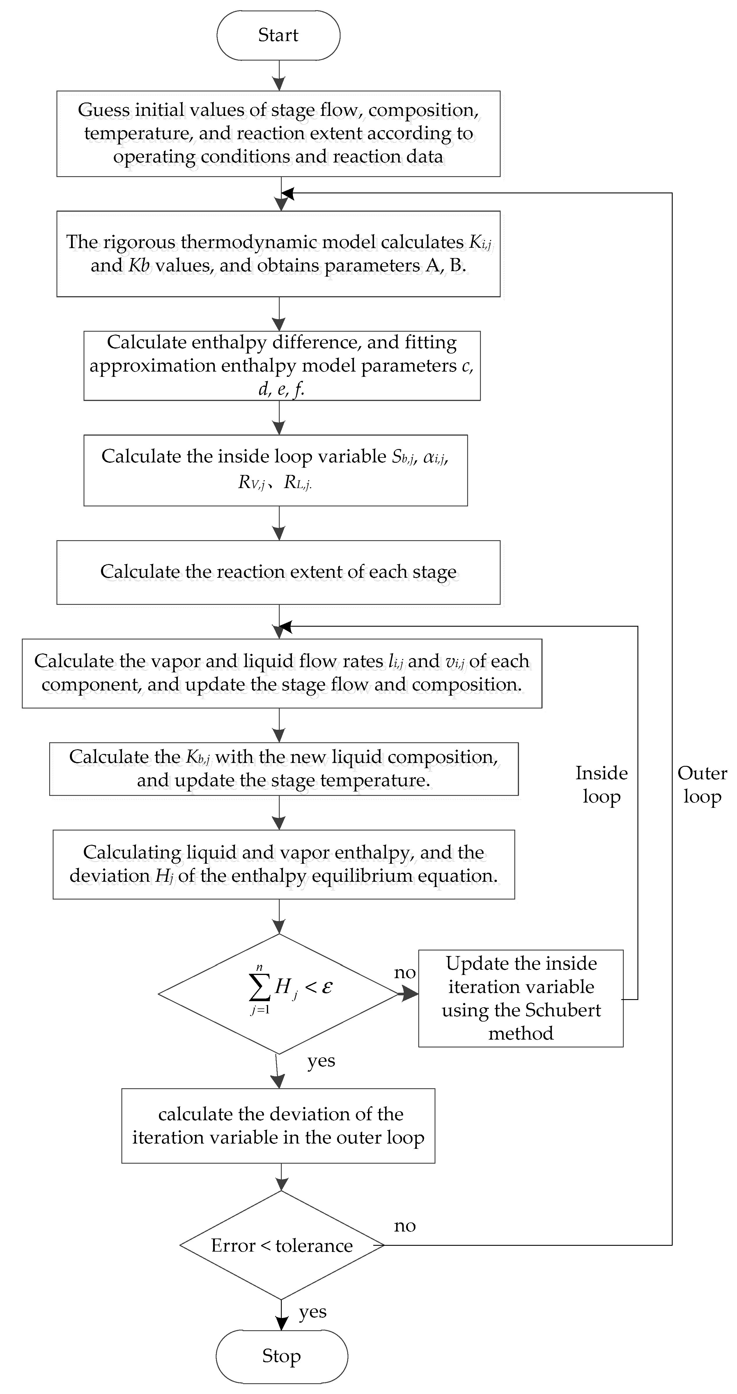
Figure 5.
Schematic diagram of the isopropyl acetate reactive distillation column.

Figure 6.
Comparison of the initial values of the extent of reaction and simulation results.

Figure 7.
Error at each iteration for the simulation of isopropyl acetate reactive distillation column.
Figure 7.
Error at each iteration for the simulation of isopropyl acetate reactive distillation column.


Table 1.
Operational conditions of the reactive distillation column.
| Variables | Specifications |
|---|---|
| Reaction section | 1218– stages |
| Condenser pressure | 0.4 atm |
| Stage pressure drop | 0.689 kPa |
| Distillate rate | 9.78 kmol·h−1 |
| Reflux ratio | 2.98 |
| Liquid holdup | 0.2 m3 |
| Condenser type | Total |
| Reboiler type | Kettle |
Table 2.
Comparison of the simulation results of Example 1.
| Variables | Simulated | Zhang et al. [6] | δ1% |
|---|---|---|---|
| Temperature of top tower/°C | 61.58 | 62.00 | 0.68 |
| Temperature of bottom tower/°C | 112.92 | 112.57 | 0.31 |
| Condenser heat duty/kW | −382.71 | −375.88 | 1.82 |
| Reboiler heat duty/kW | 312.11 | 304.58 | 2.47 |
| Distillate of top tower/kmol·h−1 | 9.78 | 9.78 | 0.00 |
Table 3.
Comparison of product composition of Example 1.
| Simulated | Zhang et al. [6] | δ1% | ||
|---|---|---|---|---|
| Mole Fraction (top tower) | IPOH | 0.0022 | 0.0023 | 4.35 |
| HAc | 0.0048 | 0.0047 | 2.13 | |
| IPAc | 0.9905 | 0.9907 | 0.02 | |
| H2O | 0.0023 | 0.0022 | 4.55 | |
| DMSO | 0.0001 | 0.0001 | 0.00 | |
| Mole Fraction (bottom tower) | IPOH | 0.0016 | 0.0017 | 5.88 |
| HAc | 0.1886 | 0.1898 | 0.63 | |
| IPAc | 0.0060 | 0.0057 | 5.26 | |
| H2O | 0.2628 | 0.2609 | 0.73 | |
| DMSO | 0.5410 | 0.5419 | 0.17 | |
Table 4.
The parameters of feed stream for the depropanization column.
| Variables | Feed 1 | Feed 2 | Feed 3 |
|---|---|---|---|
| Temperature/°C | 21.0 | 45.0 | 56.5 |
| Pressure/kPa | 3043.32 | 2200.32 | 2333.32 |
| Feed stage | 31 | 33 | 37 |
| Flow/kmol·h−1 | 42.01 | 1329.96 | 706.03 |
| Mole fraction | |||
| H2 | 0.9574 | 0.0000 | 0.0000 |
| N2 | 0.0010 | 0.0000 | 0.0000 |
| CH4 | 0.0416 | 0.0000 | 0.0000 |
| C2H6 | 0.0000 | 0.0005 | 0.0001 |
| C3H6 | 0.0000 | 0.7031 | 0.7025 |
| C3H8 | 0.0000 | 0.0266 | 0.0551 |
| C3H4-1 | 0.0000 | 0.0257 | 0.0694 |
| C4H8-1 | 0.0000 | 0.0874 | 0.0763 |
| C4H6-4 | 0.0000 | 0.1194 | 0.0950 |
| C4H10-1 | 0.0000 | 0.0025 | 0.0014 |
| C5H10-2 | 0.0000 | 0.0256 | 0.0002 |
| C6H12-3 | 0.0000 | 0.0012 | 0.0000 |
| C6H6 | 0.0000 | 0.0069 | 0.0000 |
| C7H14-7 | 0.0000 | 0.0007 | 0.0000 |
| C7H8 | 0.0000 | 0.0003 | 0.0000 |
Table 5.
Operational conditions for the depropanization column.
| Variables | Specifications |
|---|---|
| Numbers of stages | 42 |
| Reaction section | 13–stages |
| Condenser pressure | 20.2 atm |
| Stage pressure drop | 1.325 kPa |
| Bottoms rate | 854.8 kmol·h−1 |
| Reflux ratio | 0.98 |
| Condenser type | Partial-Vapor-Liquid |
| Reboiler type | Kettle |
Table 6.
Comparison of the simulation results of Example 2.
| Variables | Simulated | Measured | δ1% |
|---|---|---|---|
| Temperature of top tower/°C | 49.0 | 48.5 | 1.03 |
| Temperature of bottom tower/°C | 79.4 | 79.0 | 0.51 |
| Condenser heat duty/kW | −12,167.0 | ||
| Reboiler heat duty/kW | 11,486.7 | ||
| Distillate rare of liquid/kg·h−1 | 49,515.5 | 49,625.0 | 0.22 |
| Distillate rare of vapor/kg·h−1 | 248.7 | 255.7 | 2.74 |
| Bottoms product flow/kg·h−1 | 42,523.3 | 42,507.0 | 0.04 |
Table 7.
Comparison of the mass compositions of the product flow of Example 2.
| Component | Mass Fraction (Distillate Liquid) | Mass Fraction (Bottom) | ||||
|---|---|---|---|---|---|---|
| Simulated | Measured | δ1% | Simulated | Measured | δ2% | |
| H2 | 0.0002 | 0.0002 | 1.53 | 0.0000 | 0.0000 | 0.00 |
| N2 | 0.0000 | 0.0000 | 0.00 | 0.0000 | 0.0000 | 0.00 |
| CH4 | 0.0005 | 0.0005 | 3.42 | 0.0000 | 0.0000 | 0.00 |
| C2H6 | 0.0004 | 0.0004 | 1.57 | 0.0000 | 0.0000 | 0.00 |
| C3H6 | 0.9575 | 0.9596 | 0.22 | 0.3225 | 0.3204 | 0.66 |
| C3H8 | 0.0413 | 0.0392 | 5.36 | 0.0313 | 0.0322 | 2.80 |
| C3H4-1 | 0.0001 | 0.0000 | 0.00 | 0.0521 | 0.0502 | 3.78 |
| C4H8-1 | 0.0000 | 0.0000 | 0.00 | 0.2263 | 0.2243 | 0.89 |
| C4H6-4 | 0.0000 | 0.0000 | 0.00 | 0.2854 | 0.2873 | 0.66 |
| C4H10-1 | 0.0000 | 0.0000 | 0.00 | 0.0054 | 0.0060 | 10.00 |
| C5H10-2 | 0.0000 | 0.0000 | 0.00 | 0.0546 | 0.0564 | 3.19 |
| C6H12-3 | 0.0000 | 0.0000 | 0.00 | 0.0030 | 0.0032 | 6.25 |
| C6H6 | 0.0000 | 0.0000 | 0.00 | 0.0162 | 0.0170 | 4.71 |
| C7H14-7 | 0.0000 | 0.0000 | 0.00 | 0.0022 | 0.0022 | 0.91 |
| C7H8 | 0.0000 | 0.0000 | 0.00 | 0.0009 | 0.0009 | 7.12 |
© 2020 by the authors. Licensee MDPI, Basel, Switzerland. This article is an open access article distributed under the terms and conditions of the Creative Commons Attribution (CC BY) license (http://creativecommons.org/licenses/by/4.0/).
Share and Cite
MDPI and ACS Style
Wang, L.; Sun, X.; Xia, L.; Wang, J.; Xiang, S. Inside–Out Method for Simulating a Reactive Distillation Process. Processes 2020, 8, 604. https://doi.org/10.3390/pr8050604
AMA Style
Wang L, Sun X, Xia L, Wang J, Xiang S. Inside–Out Method for Simulating a Reactive Distillation Process. Processes. 2020; 8(5):604. https://doi.org/10.3390/pr8050604
Chicago/Turabian StyleWang, Liang, Xiaoyan Sun, Li Xia, Jianping Wang, and Shuguang Xiang. 2020. "Inside–Out Method for Simulating a Reactive Distillation Process" Processes 8, no. 5: 604. https://doi.org/10.3390/pr8050604
Note that from the first issue of 2016, this journal uses article numbers instead of page numbers. See further details here.