MobileNetV2 Ensemble for Cervical Precancerous Lesions Classification

Abstract

Women’s cancers remain a major challenge for many health systems. Between 1991 and 2017, the death rate for all major cancers fell continuously in the United States, excluding uterine cervix and uterine corpus cancers. Together with HPV (Human Papillomavirus) testing and cytology, colposcopy has played a central role in cervical cancer screening. This medical procedure allows physicians to view the cervix at a magnification of up to 10%. This paper presents an automated colposcopy image analysis framework for the classification of precancerous and cancerous lesions of the uterine cervix. This framework is based on an ensemble of MobileNetV2 networks. Our experimental results show that this method achieves accuracies of 83.33% and 91.66% on the four-class and binary classification tasks, respectively. These results are promising for the future use of automatic classification methods based on deep learning as tools to support medical doctors.

1. Introduction

It is estimated that every year, at least two million women are diagnosed with breast or cervical cancer [1]. Cervical cancer is the fourth most common women’s cancer worldwide, both in incidence and mortality, while it is the most common cancer in 38 countries [1]. Global inequities (both geographical and socio-economical) in cervical cancer incidence and mortality have long been observed [2], and they persist to this day. Consequently, women’s cancers are still a major challenge for global healthcare, especially in low and middle-income countries (LMIC) where approximately 90% of deaths from cervical cancer occur, according to the World Health Organization (WHO). In [1], it was estimated that approximately 85% of women diagnosed and 88% of women who die from cervical cancer live in an LMIC. For example, a large proportion of cervical cancers in Ethiopia are diagnosed at an advanced stage [3].

For 2020, 1,806,590 new cancer cases and 606,520 cancer deaths are projected to occur in the United States alone [4]. The three most common cancers for women in the United States are breast, lung, and colorectal. The cancer death rate in the United States rose until 1991. It then fell continuously through 2017 [4] for all common cancer types, excluding uterine cervix and uterine corpus cancers. These stagnant rates for these two types of women’s cancers can be attributed to the lack of major treatment advances [5,6]. This critical aspect, together with the fact that cervical cancer is a largely preventable disease with a known causative agent (i.e., human papillomavirus (HPV) with several major oncogenic subtypes) [7] call for the development of the early reliable detection of cervical precancerous lesions and cancer and for age-appropriate screening strategies [8].

WHO indicates that global mortality from cervical cancer can be reduced by actively applying a number of measures, including prevention, vaccination, early diagnosis, effective screening, and treatment. The screening tests to detect precancerous lesions include HPV DNA testing, cytology (Papanicolaou (Pap) testing), and visual inspection of the cervix. HPV testing is more frequently used as the primary cervical cancer screening test [9], while cytology-based screening is expensive and requires complicated training [10]. The Bethesda system (which was originally proposed in 1988 [11] and further revised in 1991, 2001, and 2014) is the most commonly accepted nomenclature for Pap smears [7].

Abnormal cells can be found after a routine Pap smear. CIN (cervical intraepithelial neoplasia, also called cervical dysplasia) is a precancerous lesion characterized by abnormal growth of the cells on the surface of the cervix. According to how much epithelial tissue is affected, CIN may be characterized [12] as:

• CIN1 (low-grade neoplasia), which is about one-third of the thickness of the epithelium.
• CIN2, which is one-third to two-thirds of the thickness of the epithelium.
• CIN3, which affects more than two-thirds of the thickness of the epithelium.

One of the goals of clinical diagnosis is to discern between normal/CIN1, and CIN2/CIN3 (or CIN2+). In [13], the authors proposed to change the terminology for HPV-associated squamous lesions of the anogenital tract to LSIL (low-grade squamous intraepithelial lesion) or HSIL (high-grade squamous intraepithelial lesion), as follows:

• CIN1 is referred to as LSIL.
• CIN2 (p16 negative, which is a high-risk HPV marker) is referred to as LSIL.
• CIN2 (p16 positive) is referred to as HSIL.
• CIN3 is referred to as HSIL.

The visual inspections of the cervix with acetic acid (VIA) and Lugol’s iodine (VILI) are an alternative to cytology, especially in LMIC. VIA is a visual inspection of the cervix after the application of 3–5% acetic acid [10]. Following the application, a precancerous lesion becomes white (acetowhite). However, an acetowhite area may also be a benign lesion, which needs to be excluded before considering a VIA-positive lesion as precancerous or cancer. VILI follows VIA and the precancerous lesions (tissues with low glycogen concentration), and cancer turn yellow after the application of Lugol’s iodine. Benign lesions need to be excluded, such as in the case of VIA. Colposcopy involves the examination of the cervix and surrounding areas under a microscope (colposcope), which is the most common procedure for visualization of the cervix before and after the application of acetic acid.

The present study applies the deep learning methodology to a cervical image dataset of 477 colposcopy cases (each case is composed of five pictures after the VIA procedure, one taken using a green lens and one after VILI) and proposes a precancerous lesion diagnosis method that is based on an ensemble of MobileNetV2 networks, which represents the first use of these networks for the automated classification of precancerous lesions. After a section dedicated to the evolution and advances in the computer-aided diagnosis of colposcopy images, this paper continues with details on the actual implementation of the proposed method and the obtained results. It ends with a section on future possible developments.

2. Related Work

In the early years of computer-aided diagnosis applied in medical imaging, there were presented several studies on the use of traditional image analysis techniques for cervical cancer diagnosis. A statistical texture analysis approach focusing on six different vascular patterns that relate to cervical lesions was shown to demonstrate a classification accuracy of over 95% [14]. A multispectral imaging system for the in vivo detection of cervical precancer and cancer, after the application of acetic acid (to enhance the reflectance differences between normal and pathologic epithelium), was developed and presented in [15] where improved sensitivity and specificity was demonstrated. ColpoCAD (a Computer-Aided-Diagnosis (CAD) system for colposcopy) was introduced in [16] as a multi-sensor, multi-data, and multi-feature colposcopy images analysis tool. For example, ColpoCAD features algorithms to assess the smoothness of a lesion margin and to detect mosaic and punctuation vessel patterns. Segmentation of macro-regions in colposcopy images was at the basis of a unified model-based image analysis framework reported in [17]. Again, the classification of vascular abnormalities was modeled as a problem of texture classification, and the major contribution of that paper was to address the detection of all vascular abnormalities in a unified framework.

In the age of data-driven machine learning techniques, biomedical imaging and analysis have been attracting a largely increasing interest from the scientific community. The application areas are very diverse, and they target various organs. For example, the use of 3D convolutional neural networks (CNNs) to discriminate between primary and metastatic liver tumors from MRI data was proposed and evaluated in [18]. In [19]; a deep CNN-based method and transfer learning were proposed for breast MRI tumor classification; and in [20], transfer learning was used for the diagnosis of lung diseases, including cancer and tuberculosis. Recently, an entire issue of the Proceedings of the IEEE was dedicated to diverse computational strategies based on deep learning for the analysis of medical images [21]. In [22], a survey on using deep learning techniques (mainly CNNs) for medical images analysis was given and presented over 300 contributions to the field (mainly in image classification, but also in object detection, segmentation, and registration). Cervical dysplasia diagnosis was included in the application areas.

Multimodal deep learning for cervical dysplasia diagnosis was presented in [23] where the results of using a CNN indicated 87.83% sensitivity at 90% specificity on a large dataset. Another CNN-based method for localized classification of uterine cervical cancer histology images was presented in [24], where the accuracy of 77.25% was reported.

In [25], from a total of 485 images in the dataset (from 157 patients), a total of 233 were captured with a green filter, and the remaining 252 were captured without a green filter. Of the total number of images, 142 images were of severe dysplasia, 257 of CIS (carcinoma in situ), and 86 of invasive cancer. The training was performed using Keras and TensorFlow. The accuracy obtained was approximately 50%.

In [26], images from 330 patients who underwent colposcopy were analyzed (97 patients were diagnosed with LSIL and 213 with HSIL). A CNN with 11 layers was used, and the accuracy and sensitivity for diagnosing HSIL were 0.823 and 0.797, respectively.

A mobile phone application to be used in low-income settings, dedicated to the preliminary analysis of the digital images of the cervix (after VIA), was presented in [27].

Cell morphology was combined with cell image appearance for the classification of cervical cells in Pap smear in a CNN-based approach in [28]. The dataset used was the Herlev benchmark Pap smear on which four CNN models (AlexNet, GoogLeNet, ResNet, and DenseNet) pretrained on the ImageNet dataset were fine-tuned. For the two-class and the seven-class classification tasks, GoogLeNet obtained the best accuracies, 94.5% and 64.5%, respectively.

The first study to use transfer learning with the DenseNet model (ImageNet and Kaggle) for the classification of colposcopy images was presented in [29] where the accuracy of 73.08% in 600 test images was reported.

Other machine learning techniques have been used for cervical disease diagnosis as well. In [30], several cervigram images from the U.S. National Cancer Institute were collected and further enhanced to evaluate image-based cervical disease classification algorithms. Further, to differentiate between high-risk and low-risk patients, seven classic machine learning algorithms (random forest (RF), gradient boosting decision tree (GBDT), AdaBoost, support vector machines (SVM), logistic regression (LR), multilayer perceptron (MLP), and k-nearest neighbors (kNN)) were trained and tested on the same datasets on a ten-round ten-fold cross-validation. The RF algorithm was shown to yield the best results with accuracy, sensitivity, and specificity of 80%, 84.06%, and 75.94%, respectively. RF was also used in [31] where image segmentation for cervigrams was the first step of the approach. The method’s next steps were the extraction of color and texture features for the interpretation of uterine cervix images. Next, the Boruta algorithm was applied for feature selection. The final step involved the use of RF.

The present paper is the first to propose the use of MobileNetV2 [32] networks for the automatic classification of colposcopy images. We used a diverse input composed of three different types of images: from VIA, from a green lens, and from VILI. Another contribution of this paper is the modeling of the ensemble, which is built from several MobileNetV2 sub-networks and an inverted residual unit (a stack of convolutional layers specific to the MobileNetV2 architecture). The sub-networks transform the different images into three-dimensional embeddings that capture the discriminative features for the problem of CIN classification. The inverted residual unit processes the embeddings from multiple images in order to find distinctive patterns. Apart from the network modeling, we directed our research towards handling class imbalance, which is common in this domain, and manipulated the loss function, to be more robust to this phenomenon. Last, to better understand the functioning of the network, we visualized its activations and identified problem areas.

3. Materials and Methods

3.1. Dataset Description and Data Augmentation

We used the IEEE Dataport cervigram image dataset [33], which consists of images from colposcopy procedures. As mentioned in the Introduction, during the procedure, an acetic acid solution is applied to the cervix area to help the doctor to better visualize abnormal regions. After the application of the solution, the areas of interest will change color, becoming white. There are seven images for each medical visit: five of them contain sequential pictures of the cervix after applying the acetic acid solution, one views the cervix through a green lens, and one displays the cervix after applying iodine solution [33], a solution of a dark red color. The images are ordered as follows: the five involving acetic acid solution are first; next is the image through the green lens; and last is the image having iodine solution, as presented in Figure 1. The dataset was constructed in such a way that if we sorted the image files alphabetically, then in each folder, we obtained this ordering of images. However, there were a few exceptions to this rule, and in those cases, we renamed the files so that they were sorted properly. The data were classified into four categories [33]: normal cervix (class label 0), CIN1 (class label 1), CIN2/3 (class label 2), and cervical cancer (class label 3).

The dataset available at [33] contained a training set and a test set. We used the same train/test images as proposed by the authors in [33]. The dataset contained 3339 images of a size of $480\times 640$ pixels, of which 3003 belonged to the training set and 336 belonged to the test set. However, the data variety was limited because the pictures belonged to only 477 medical visits, and many of the images were similar. The images were grouped per visits, so we knew to which visit each image belonged. The training set and test set contained separate patient visits; thus, images from the same visit would never get mixed into both the training set and the test set. This was an important observation since we needed a model that generalized well to novel patients.

Data augmentation plays a very important role in combating overfitting, especially when dealing with lower volumes of data.

Table 1. Image transformations used for dataset augmentation.

Transformation	Parameters
Rotation	random between $0^{°}$ and ${45}^{°}$
Scale	random between 100 and 200%
Shear	random between $0^{°}$ and ${30}^{°}$
Resize	$224\times 298$ pixels
Horizontal flip	random 50%
Normalization	mean = [0.485, 0.456, 0.406];   std = [0.229, 0.224, 0.225];  tensors represent RGB dimensions

presents the image transformations that we used for augmentation. The parameters for each transformation were picked randomly between established bounds; therefore, each training sample was unique.

3.2. Model Description

3.2.1. MobileNetV2 Architecture and Concepts

In the current work, we propose an ensemble of MobileNetV2 [32] networks as a solution to the problem of colposcopy images’ classification. The choice of the MobileNetV2 architecture was motivated by several reasons. The dataset in use was relatively small for training a network on the task of visual recognition, making it prone to overfitting, while using a smaller, but expressive network such as the MobileNetV2 countered this effect. The MobileNetV2 is an architecture that optimizes memory consumption and execution speed at a low cost in terms of error [32]. The fast execution speed makes experimenting and parameter tuning much easier, while the low memory consumption is a desirable quality in the context of an ensemble of networks. Two of the most important concepts describing the MobileNetV2 architecture are the depthwise separable convolution [32] and the inverted residual [32], which will be further discussed.

As described in [32], the depthwise separable convolution is used in other efficient models, such as MobileNets [34], Xception [35], and ShuffleNet [36]. Depthwise separable convolution substitutes conventional convolution with two operations [32]. The first operation is a feature map-wise convolution; that is, a separate convolution is applied to each feature map [32]. The resulting feature maps are stacked together, and they are processed by the second operation, which is a pointwise convolution [32]. The pointwise convolution has a $1\times 1$ kernel, and it is applied to all of the feature maps at the same time [32]. A conventional convolution processes the image across the width, height, and channel dimensions at the same time. Meanwhile, the depthwise separable convolution processes the image by the width and height dimensions during the first operation and across the channel dimension during the second operation, being a factorization of the conventional convolution [32]. As described in [32], the computational costs of conventional convolution $C_{normal}$ and depthwise separable convolution $C_{separable}$ are:

$$C_{normal}=h_i·w_i·d_i·d_j·k^2.$$

(1)

$$C_{separable}=h_i·w_i·d_i(d_j+k^2).$$

(2)

$C_{normal}$	cost of conventional convolution;
$C_{separable}$	cost of depthwise separable convolution;
i	input layer index;
j	output layer index;
$h_i$	height of input feature maps;
$w_i$	width of input feature maps;
$d_i$	number of input feature maps;
$d_j$	number of output feature maps;
k	filter size.

By dividing (1) with (2), one can quantify the computational advantage of using depthwise separable convolutions over conventional convolutions [32]:

$$\frac{C_{normal}}{C_{separable}}=\frac{d_j·k^2}{d_j+k^2}.$$

(3)

In [32], the inverted residuals were described and compared to residual blocks [37], which are an important component of the ResNet model [37]. Both blocks use bottlenecks and residual connections [32], and both use three convolutional operators [32,37]. The first and last operators use $1\times 1$ filters [32,37], which transform data from the input domain to an intermediate representation and the intermediate representation to the output domain. The intermediate representation is processed by a $3\times 3$ filter [32,37]. In the residual block, the first and last convolutions have more feature maps (channels) compared to the inner convolution of the block [37]; in contrast, the inverted residual uses the first and last convolutions with a smaller number of feature maps compared to the inner convolution [32]. In both cases, the residual connection is between the first and last feature maps, which are less in the case of MobileNetV2 [32] when compared to ResNet [37]. In both architectures, if we stack multiple units, it results an alternation of larger and smaller layers. The essential difference lies in the placement of the residual connections, which brings an advantage in terms of memory consumption in the MobileNetV2 architecture [32].

We used a publicly available implementation of the MobileNetV2 network from the PyTorch Hub [38]. All the MobileNetV2 network implementation details are found at [38] and in the MobileNetV2 paper [32], while the source code is also publicly available at the GitHub link [39].

Table 2. Generic information related to the MobileNetV2 architecture [32]. In the details below, we took into account the implementation in [38].

Network depth	The network contains 17 inverted residual units stacked between two convolutional layers and a single fully connected layer. Given that each inverted residual block is implemented using three convolutional layers, we can conclude that the network has a depth of 53 convolutional layers and a single fully connected layer.
Filter size	All depthwise separable convolutions are implemented using two convolutions; the first has a $3\times 3$ filter size, while the second has a $1\times 1$ filter size. The depthwise separable convolutions are better explained in Section 3.2.1. The other two regular convolutional layers that act as adapters for the input and output representations have a filter size of $3\times 3$ and $1\times 1$.
Spatial downsampling	The spatial downsampling is achieved through increasing the stride to a value of two in some of the convolutional layers, while all other layers keep a stride of one. There is no maximum pooling involved.
Convolution padding	The implementation employs the padding scheme of $padding=(filter-1)/2$, as can be noted in the source code [39]. This scheme preserves the size of the layer for odd filter sizes (in our case, the network utilizes only filters of sizes of one and three).
Nonlinearities	Unlike other networks, the nonlinearity used in the MobileNetV2 network is ReLU6 instead of ReLU (rectified linear unit). While the ReLU function equals $f\left(x\right)=max(0,x)$, the ReLU6 function equals $f\left(x\right)=min(6,max(0,x\left)\right)$. According to the MobileNetV2 paper [32], the reason for using ReLU6 is that it is more robust to low precision computation.
Normalization	All convolutional operations are followed by per channel batch normalization, that is, for each batch, the layer activations are standardized to zero-mean and unit variance and then go through a linear transform parameterized by learnable scale and shift parameters.
Dropout	The network presented at [38] uses dropout only for the fully connected layer with a 20% probability of ignoring connections.

documents additional high-level features related to the MobileNetV2 network used. In the next subsection, we present an essential structural modification that we performed to this network for adapting it to our problem.

3.2.2. MobileNetV2 Tuning

The MobileNetV2 network is a series of inverted residual blocks stacked between two convolutions [32], which we can view as adapters transforming the input to an intermediary representation and the intermediary representation to output. The convolution’s final output is passed through a global average pooling layer and through an inference layer [32]. The MobileNetV2 network is adapted to the ImageNet classification challenge [40], which is a classification problem having 1000 classes. For this reason, the last convolutional layer (just after the last inverted residual block) is larger, having 1280 feature maps and a filter size of $1\times 1$ [32]. However, the cervical lesion classification problem has only four classes. Consequently, it makes sense to use a smaller representation of the image. In Section 4.1, we show that using a smaller representation achieved a better accuracy of the network regardless of being used in the context of an ensemble or alone. To constrain the size of the representation, we modified the last convolutional layer, just after the last inverted residual block, to output 32 or 64 feature maps instead of 1280. If used inside the ensemble, then this layer becomes the final layer, and the resulting feature maps are joined by those from other models and processed by the ensemble network. If the model is used alone, then the feature maps of this layer pass through global average pooling and result in a vector of 32/64 elements. The vector is further processed by a fully connected layer to calculate the result. Because the original MobileNetV2 model was pretrained on ImageNet [40], we kept all other layers unchanged to preserve the already trained parameters, and we fine-tuned the whole network during training.

3.2.3. MobileNetV2 Ensemble

The main contribution of this study is the creation of the MobileNetV2 ensemble and the tuning of the MobileNetV2 architecture to be better used in the context of the ensemble. As described in Section 3.1, the dataset could be split according to three categories: images after applying the acetic acid solution, images viewed through a green lens, and images after applying the iodine solution. In Section 4.2, we will show that training a single MobileNetV2 model on a single category of images yields better results than training on all of the categories at the same time. Based on this observation, we trained a separate model on each of the image categories. In the final step, we joined the trained models in an ensemble that yielded superior results to any of the separately trained models. We used the model described in Section 3.2.2 as the building block of our ensemble. We trained three models of this kind on the three categories of images. Each model was trained in isolation on its specific image category, and the model parameters remained fixed when the ensemble was trained. From each of the three models, we dropped the last inference layer and the average pooling, the restricted size convolution becoming the output layer. All of the feature maps resulting from the three networks were stacked and then processed by an inverted residual block that analyzed and related all images at the same time. Finally, the feature maps went through global average pooling and through a fully connected layer that calculated the result.

3.3. Network Forward Pass

This section describes a forward pass of the data through the ensemble. The network input consisted of seven images, which represented a specific colposcopy procedure. The first five images displayed the cervix after applying the acetic acid solution, while the last two displayed the cervix through a green lens and after applying the iodine solution. The ensemble contained three models, each being specialized in a certain type of image. The steps below describe the ensemble forward pass; the tensor sizes will be displayed in the form: $feature$$maps\times height\times width$.

• Every image was processed by the appropriate specialized network. The network trained on acetic acid solution images would process five images, while the other two networks would process one image each. Images were fed to the network as tensors of size $3\times 224\times 298$. The network specialized in green lens images output tensors of size $64\times 7\times 10$. The other two networks output tensors of size $32\times 7\times 10$.
• All resulted feature maps were stacked, forming a tensor containing $32\times 5+64+32=256$ feature maps; that is, a tensor of size $256\times 7\times 10$.
• The tensor was processed by an inverted residual block, as described in Section 3.2.1. The result had the shape: $32\times 7\times 10$.
• Next, global average pooling was performed, transforming the tensor of size $32\times 7\times 10$ into a tensor of size 32; that is, each feature map was averaged.
• To calculate the final result, the vector was passed through a fully connected layer, yielding a tensor of size 4.

These steps are shown in pseudocode in Algorithm 1. The pseudocode is similar to the actual PyTorch implementation. Figure 2 illustrates the forward pass and the architecture of the ensemble. The tensor transformations are summarized in

Table 3. Tensor sizes during a network run. The tensor sizes are displayed in the form: $feature$$maps\times height\times width$. The batch size is ignored.

Operation	Input Tensor	Output Tensor
MobileNetV2 CNN specialized on images with acetic acid solution	$3\times 224\times 298$	$32\times 7\times 10$
MobileNetV2 CNN specialized on images through the green lens	$3\times 224\times 298$	$64\times 7\times 10$
MobileNetV2 CNN specialized on images with iodine solution	$3\times 224\times 298$	$32\times 7\times 10$
Concatenation (receives a list of tensors)	−	$256\times 7\times 10$
Inverted residual block	$256\times 7\times 10$	$32\times 7\times 10$
Global average pool	$32\times 7\times 10$	32
Fully connected	32	4

.

Algorithm 1 Ensemble forward pass. The function parameter x is an array of seven input images. All $CNN$ are functions denoting the forward pass of a specialized convolutional neural network. The $CONCATENATE$ function stacks multiple feature maps, which have the same width and height; for example, stacking two tensors having $feature$$maps\times height\times width$ equal to $32\times 7\times 10$ will result in a tensor of size $64\times 7\times 10$. $AVG\_POOL$ calculates the average per feature map; for example, pooling a tensor of size $64\times 7\times 10$ results in a tensor of size 64. $FULLY\_CONNECTED$ is a function representing the forward pass of a fully connected layer. The resulting tensor is of size 4. Please note that, for simplicity, we did not take into account the batch dimension for tensor sizes.

functionforward(x)  $list=$ [ ]  for $i=0,\cdots 4$ do   $x_{aceticacid}=CN{N}_{aceticacid}\left(x\left[i\right]\right)$   $list.append\left(x_{aceticacid}\right)$  end for  $x_{greenlens}=CN{N}_{greenlens}\left(x\left[5\right]\right)$  $list.append\left(x_{greenlens}\right)$  $x_{iodinesolution}=CN{N}_{iodinesolution}\left(x\left[6\right]\right)$  $list.append\left(x_{iodinesolution}\right)$  $x_{concat}=CONCATENATE\left(list\right)$  $x_{invertedresidual}=CN{N}_{invertedresidual}\left(x_{concat}\right)$  $x_{averaged}=AVG\_POOL\left(x_{invertedresidual}\right)$  $result=FULLY\_CONNECTED\left(x_{averaged}\right)$  return $result$ end function

3.4. Handling of Imbalanced Datasets

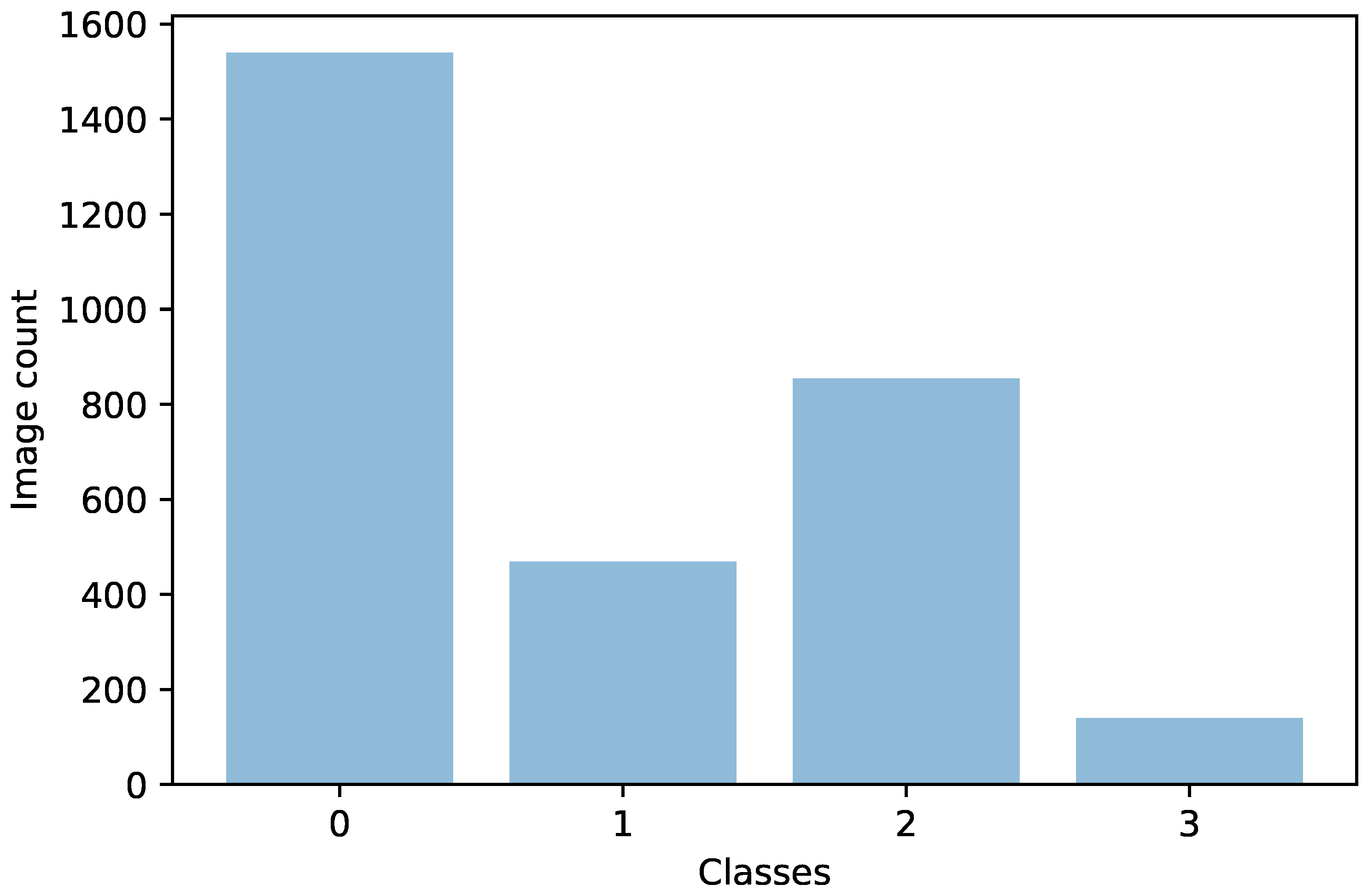
As can be observed in Figure 3, the distribution of the training samples was imbalanced among the four classes, approximately half of the samples belonging to Class 0 (normal), and under 5% to Class 3 (cancer). In this section, we describe the effect of class imbalance on the model performance and experiment with three strategies to better handle it. For all of the experiments described in this section, we used a single MobileNetV2 model tuned as described in Section 3.2.2 and only on the images involving acetic acid solution. If the metrics used were influenced by the class-specific population size, then we could get misleading results; for example, if a dataset contained 99% healthy patients and we tried to detect unhealthy ones, a model that always classified a patient as healthy would have a misleading score of 99% accuracy. Another option was to calculate the metrics separately per each class and then average. However, this could also be problematic in scenarios where there is an important class with low performance and multiple other less important classes with higher performance. In both cases, through measurement, the score of the model could get boosted artificially. We believe that the most precise view was obtained by investigating the performance of each class separately.

We chose a very simplistic metric, the true positive rate, which is also known as recall. Averaged across the four classes, this metric would not be descriptive enough to study the effects of class imbalance. However, if calculated separately for each class, then it enabled us to detect if the model became biased in recognizing certain classes to the detriment of others due to the training population structure. The per-class true positive rate was given by the percentage of true positives in the population having as ground truth that class; that is, we divided the true positives by true positives plus false negatives with respect to a certain class. We calculated the true positive rate by investigating the confusion matrix for the validation set. Given a confusion matrix M, the element $M_{i,j}$ counts the elements labeled with class i, but predicted as class j. Equation (4) presents a confusion matrix; the diagonal bold elements are true positives, and the rest are misclassifications. Each row of the matrix presents the population belonging to a certain class. Equation (5) shows the formula for calculating the true positive rate $tp{r}_i$ for class i. Given that the true positive rates were expressed as percentages, the measurements were agnostic of the number of elements contained in each class.

$$M=\left[\begin{array}{cccc}{\mathbf{m}}_{\mathbf{1},\mathbf{1}}& m_{1,2}& m_{1,3}& m_{1,4}\\ m_{2,1}& {\mathbf{m}}_{\mathbf{2},\mathbf{2}}& m_{2,3}& m_{2,4}\\ m_{3,1}& m_{3,2}& {\mathbf{m}}_{\mathbf{3},\mathbf{3}}& m_{3,4}\\ m_{4,1}& m_{4,2}& m_{4,3}& {\mathbf{m}}_{\mathbf{4},\mathbf{4}}\end{array}\right]$$

(4)

$$tp{r}_i=\frac{m_{i,i}}{{\sum }_{j=1}^4{m}_{i,j}}$$

(5)

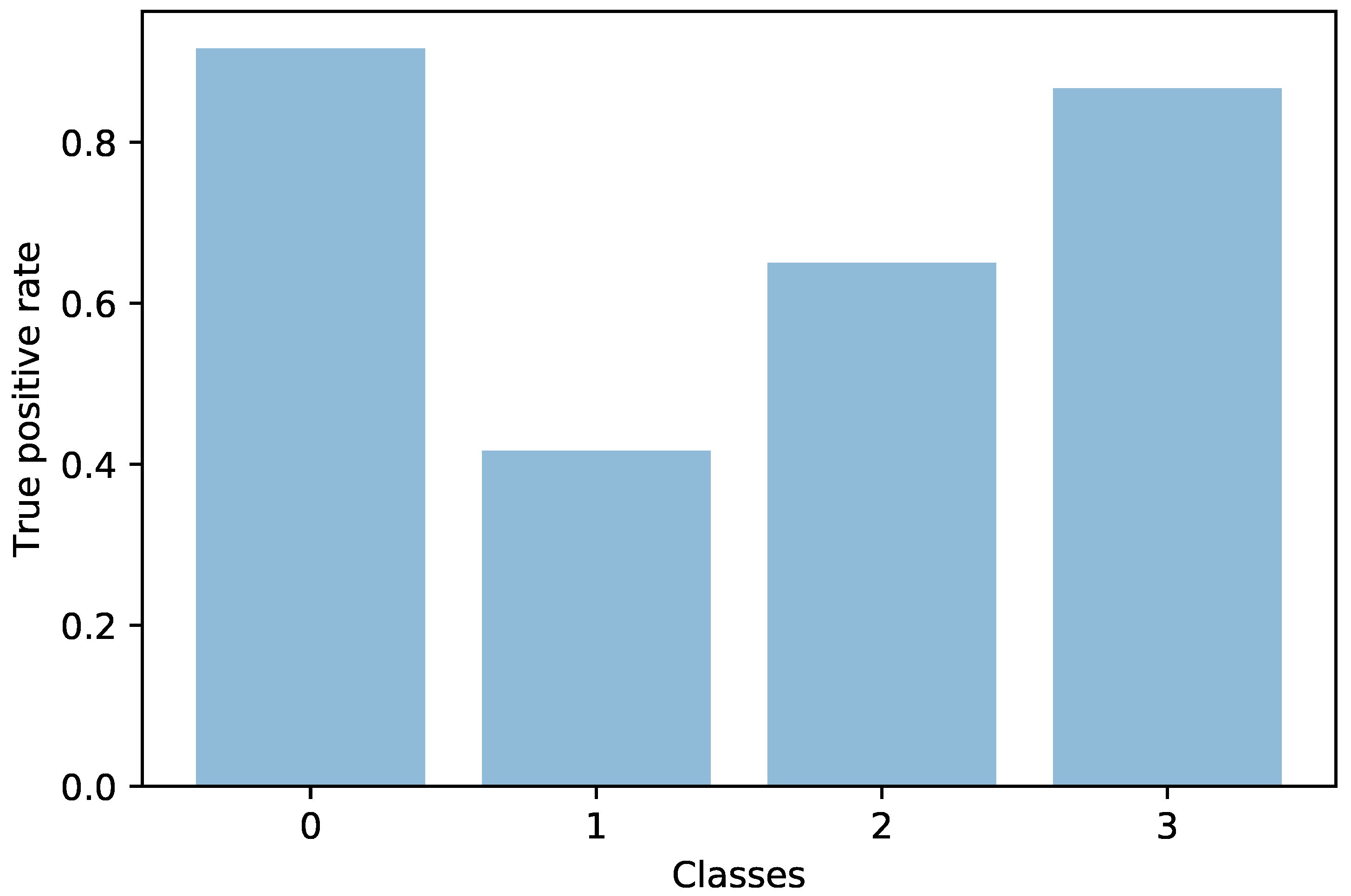
The results on the acetic acid images are depicted in Figure 4. Looking at both training data distribution and class recall, we could make the following observations:

• Class 0 had the most samples and achieved the highest true positive rate.
• Class 3 (cancer) yielded good results compared to the other classes, despite the reduced number of samples. This class was probably easier to distinguish from the others because of its distinctive visual features.
• Both Classes 1 and 2 had a smaller number of samples compared to Class 0, and a lower true positive rate.
• Class 1 had fewer samples than Class 2 and also a lower true positive rate.

Based on these observations, we noticed that except for Class 3, the amount of training samples correlated with the class true positive rate. Based on this finding, we presumed that the model would perform better if presented with a higher volume of training data. The diversity of the samples was also important.

3.4.1. Loss Function

Because of the dataset imbalance, the trained model might be biased to better recognize certain classes to the detriment of others. This happens because during training, the model is exposed to an uneven number of samples from the different classes; therefore, the model parameters are more updated in a certain direction. To counter this phenomenon, we made the model focus more on the detrimental classes during training. This could be achieved by manipulating the loss function. By default, we trained the model using the cross entropy loss, shown in Equation (6). The weighted cross entropy loss, depicted in Equation (7), uses a weight vector $\overrightarrow{\mathbf{w}}$ to put more importance on some of the classes. In the focal loss [41], the easier examples are decayed using a factor ${(1-P\left(\overrightarrow{{\mathbf{x}}_{\mathbf{i}}}\right))}^{\gamma }$, as shown in Equation (8).

$$E_{\overrightarrow{\mathbf{x}},\overrightarrow{\mathbf{y}}}=-\sum _i^N\overrightarrow{{\mathbf{y}}_{\mathbf{i}}}ln\left(P\left(\overrightarrow{{\mathbf{x}}_{\mathbf{i}}}\right)\right)$$

(6)

$$W{E}_{\overrightarrow{\mathbf{x}},\overrightarrow{\mathbf{y}},\overrightarrow{\mathbf{w}}}=-\sum _i^N\overrightarrow{{\mathbf{y}}_{\mathbf{i}}}[\overrightarrow{\mathbf{w}}\odot ln\left(P\left(\overrightarrow{{\mathbf{x}}_{\mathbf{i}}}\right)\right)]$$

(7)

$$F_{\overrightarrow{\mathbf{x}},\overrightarrow{\mathbf{y}}}=-\sum _i^N\overrightarrow{{\mathbf{y}}_{\mathbf{i}}}[{(1-P\left(\overrightarrow{{\mathbf{x}}_{\mathbf{i}}}\right))}^{\gamma }\odot ln\left(P\left(\overrightarrow{{\mathbf{x}}_{\mathbf{i}}}\right)\right)]$$

(8)

$E_{\overrightarrow{\mathbf{x}},\overrightarrow{\mathbf{y}}}$	cross entropy loss function;
$W{E}_{\overrightarrow{\mathbf{x}},\overrightarrow{\mathbf{y}},\overrightarrow{\mathbf{w}}}$	weighted cross entropy loss function;
$F_{\overrightarrow{\mathbf{x}},\overrightarrow{\mathbf{y}}}$	focal loss function;
$\overrightarrow{\mathbf{x}}$	list containing network input tensors;
$\overrightarrow{\mathbf{y}}$	list containing one-hot-vectors indicating the ground truths;
$\overrightarrow{\mathbf{w}}$	four-dimensional vector of class weights;
N	number of training samples;
i	index through the training samples;
$P\left(\overrightarrow{{\mathbf{x}}_{\mathbf{i}}}\right)$	function outputting a four-dimensional vector with the probabilities of input $\overrightarrow{{\mathbf{x}}_{\mathbf{i}}}$ to belong to each of the classes; obtained by running a forward pass through the network with input $\overrightarrow{{\mathbf{x}}_{\mathbf{i}}}$ and applying softmax;
$ln$	natural logarithm;
$\gamma$	scalar decaying the loss for easier examples;
⊙	element-wise multiplication between two vectors; that is, element i from the first vector gets multiplied by element i from the second vector, and the result vector has the same dimensions as the product factors.

As noted in Equation (6), the simple cross entropy loss already has a mechanism for countering the class imbalance. The network does not learn at the same rate from all examples. As the probability $P\left(\overrightarrow{{\mathbf{x}}_{\mathbf{i}}}\right)$ goes to one, the logarithm goes to zero. Therefore, as the model gets more confident, the learning saturates.

The weighted cross entropy loss is useful when some classes are more important than others or need more attention during training. We experimented with two variants: one in which we kept the class weights $\overrightarrow{\mathbf{w}}$ fixed according to population size and the other in which the class weights $\overrightarrow{\mathbf{w}}$ were recalculated after each epoch, based on the class error rates. The error rate $e_{t,i}$ for epoch t and class i is one minus the true positive rate:

$$e_{t,i}=1-tp{r}_{t,i}$$

(9)

The error rate is also equal to the sum of false negatives for a certain class. We applied a transformation $\varphi$ to each error rate $e_{t,i}$ to provide more importance to higher error rates. The class weights are calculated following Equation (10).

$$w_{t,i}=\frac{\varphi \left(e_{t,i}\right)}{{\sum }_j^4\varphi \left(e_{t,j}\right)}$$

(10)

If we set $\varphi \left(x\right)=x$ (i.e., the identity function), then the weights would be directly proportional to the error rates. If we set $\varphi \left(x\right)=exp\left(x\right)$, then we would get the softmax function. In our experiments, we set $\varphi \left(x\right)$ to $x^3$, $exp\left(x\right)$, $exp\left(10x\right)$, and $exp\left(100x\right)$. On each epoch, the loss function puts more focus on the needed classes. This was more efficient when we trained for a longer period and progressed slowly. Consequently, we used a smaller learning rate of ${10}^{-5}$ compared to ${10}^{-4}$ used during normal training.

The focal loss distributes its attention at an even more granular level than the weighted cross entropy loss. Instead of focusing on a certain class, the focal loss uses different weights for each training sample regardless of the class to which it belongs.

3.4.2. Conclusions on Handling Class Imbalance

From our experiments, as detailed in Section 4.4, we note that the weighted cross entropy loss with dynamic weighting on each epoch and a $\varphi \left(x\right)=exp\left(100x\right)$ worked best and provided a better balanced model, as can be observed in Figure 5. We extended this approach to the other images, but it only offered benefits in the case of those with acetic acid and those through the green lens. In the case of iodine solution images, the performance of the model degraded. Next, we constructed an ensemble from the models trained with weighted cross entropy for acetic acid and green lens images, while keeping the normally trained model for iodine solution images. The ensemble showed the same performance as the one built from the classical models (i.e., trained with simple cross entropy); therefore, it might be possible that the ensemble has a positive impact on class imbalance.

3.5. Implementation Details

3.5.1. Network Evaluation

We measured the accuracy, recall, precision, and F1 score. Recall, precision, and F1 score are metrics used for binary classification; however, they were adapted to multiple class problems by using a one versus rest approach; that is, if an instance contained the class in question, it was considered positive; if it contained any other class, it was considered negative; the results calculated on the four classes were averaged. The researcher can choose to average using equal weighting or a weighting according to the size of the population of each class. For our problem, we chose equal weighting. As noted in Section 3.4, most of the images displayed normal cervices that were easily distinguished by the model. If we weighted according to population size, then we would get an overly optimistic result.

3.5.2. Training Details

We used an Adam optimizer with ${\beta }_1=0.9,{\beta }_2=0.999$, $ϵ={10}^{-8}$, $weight\_decay=0$. The learning rate was set to ${10}^{-4}$ for training the individual MobileNetV2 networks and the ensemble. The networks were trained in isolation and kept fixed weights while training the ensemble. For the experiments related to the handling of dataset imbalance, the learning rate was modified to ${10}^{-5}$ for those trained with weighted cross entropy and ${10}^{-3}$ for those trained with focal loss. During training with weighted cross entropy loss, most attention was directed to certain classes each epoch, while others received little training. To assure convergence, we recommend a smaller learning rate. For focal loss, we recommend a higher learning rate because the focal objective diminishes the intensity of the network updates. We trained for a predefined number of iterations, which was specific to each problem. The number of iterations was set to a higher value than necessary so that the model entered the overfitting zone. The state of overfitting was assessed visually by the developer by plotting the loss and the other metrics on both training and test sets. While training, each time that the accuracy on the test set increased, a new checkpoint of the model was saved. Thus, at the end of the training, we were left with the best version of the model that found the equilibrium between underfitting and overfitting. For the experiments on dataset imbalance handling, instead of accuracy, we used the harmonic mean of the per-class true positive rate as a criterion for saving model checkpoints, and we will describe this in more detail in Section 4.4.

3.5.3. Ensemble Inverted Residual

The ensemble inverted residual unit is especially important because it analyzes all images at once. As described in [32], the “expansion ratio” is the ratio between the number of feature maps used by the inner layer of the inverted residual and the number of feature maps used by the input (bottleneck) layer. We used an expansion ratio of 5; thus, the inner convolutions of the inverted residual had $5\times 256=1280$ feature maps. As an additional regularization technique, we added two dropout layers inside the inverted residual unit after the input convolution and the internal convolution, each having a drop probability of 60%.

Table 4. Ensemble inverted residual unit design.

Layer Type	Parameters
Convolution	input feature maps = 256;  output feature maps = 1280;  filter size = 1
Batch normalization	-
ReLU	-
Dropout	60% drop probability
Convolution	input feature maps = 1280;  output feature maps = 1280;  filter size = 3
Batch normalization	-
ReLU	-
Dropout	60% drop probability
Convolution	input feature maps = 1280;  output feature maps = 32;  filter size = 1
Batch normalization	-

summarizes the structure of the inverted residual. For fine-tuning the ensemble, we reduced the learning rate to ${10}^{-8}$ and the dropout drop probability from 60% to 20%.

4. Results

4.1. MobileNetV2: Comparison with Other Networks and Parameter Tuning

We chose the following models as baselines: VGG19 [42], ResNet18 [37], DenseNet [43], ResNeXt-101 [44], and MobileNetV2 [32]. All models were pretrained on ImageNet [40], and ResNeXt was additionally trained in a weakly supervised manner on 940 million public images [44]. We fine-tuned those models on the images involving acetic acid solution. In our work, we tuned the MobileNetV2 architecture to better fit the current problem as described in Section 3.2.2 and compared it to the baselines as shown in

Table 5. Baselines and tuned MobileNetV2 metrics measured on the acetic acid images.

Model	Accuracy	Precision	Recall	F1 Score
DenseNet	63.75%	55.26%	39.20%	43.61%
ResNet18	64.16%	44.54%	34.04%	37.40%
MobileNetV2	64.58%	45.03%	35.48%	38.04%
ResNeXt-101	64.58%	48.30%	35.41%	39.04%
VGG19	68.75%	49.26%	40.74%	44.42%
MobileNetV2 tuned (ours)	71.24%	66.39%	52.70%	57.69%

. The metrics between ResNet18, MobileNetV2, and ResNeXt-101 were very close to one another, even though the size and depth of each of those networks were very different. Normally, we would expect the ResNeXt-101 model to outperform the others by a larger margin, but we believe that it was a too complex model to be applied to a dataset of this size. From the baselines, VGG19 performed the best. We believe that the results could be explained by the capability of each network to fight overfitting: VGG19 had two dropout layers with a 50% probability of dropping activations from the fully connected layers, while the other networks had less aggressive dropout or were entirely missing it. The increase in performance from our model came from its ability to counter overfitting. We addressed this by using a pretrained model, by diminishing the size of the last convolutional layer from 1280 to 32 filters, as explained in Section 3.2.2, and by adding after the last convolution an aggressive two-dimensional dropout layer with a 70% probability of dropping connections. As explained in Section 3.5.3, the ensemble inverted residual also presented two dropout layers, each having a 60% chance to drop a connection while training.

4.2. Training on Different Image Types

After testing our tuned MobileNetV2 network on images with acetic acid solution, we extended to images through the green lens and with iodine solution. We ended up having three networks specialized in each type of image. If we trained a single network on all types of images, then we obtained a lower performance than from any of the specialized networks, which further supported the need for an ensemble that could take advantage of all image types at once. A possible explanation is that it is easier to compare two instances that shared the same context than comparing two instances belonging to different contexts. In our case, the types of images, acetic acid, green lens, and iodine solution, were the context, and each image was an instance. Moreover, the image types were very different from one another, and the ratio of acetic acid images was much bigger than the others. Thus, when training on all image types at the same time, green lens and iodine solution images turned into noise instead of being useful. We used the three specialized models to build an ensemble, which in turn outperformed all specialized networks. We also turned our system into a binary classifier, in which Classes 0 and 1 (normal and CIN1, respectively) were considered 0 and Classes 2 and 3 (CIN2/3 and cancer, respectively) were considered 1. We did not perform any additional training or model changes for this task; we simply used the four-class model and recorded the metrics as if we had a binary problem.

Table 6. Results of the network trained on all images at once, of networks specialized on individual image types and of the ensemble in both four class and binary mode. For the ensemble, we provide a simpler version and another one fine-tuned through training with a smaller learning rate. Where we mention MobileNetV2, we refer to the model modified as described in Section 3.2.2.

Model	Accuracy	Precision	Recall	F1 Score
MobileNetV2 trained on all image types	63.98%	45.45%	38.27%	40.39%
MobileNetV2 trained on acetic acid images	71.24%	66.39%	52.70%	57.69%
MobileNetV2 trained on green lens images	75.00%	81.80%	75.00%	75.24%
MobileNetV2 trained on iodine solution images	75.00%	79.80%	75.00%	74.62%
Ensemble, four class mode	81.25%	85.04%	81.25%	81.20%
Ensemble, binary classification mode	89.58%	89.65%	89.58%	89.57%
Ensemble fine-tuned, four class mode	83.33%	86.41%	83.33%	83.55%
Ensemble fine-tuned, binary classification mode	91.66%	91.66%	91.66%	91.66%

presents the results of the ensemble and compares it to the specialized networks and the network trained on all images at once.

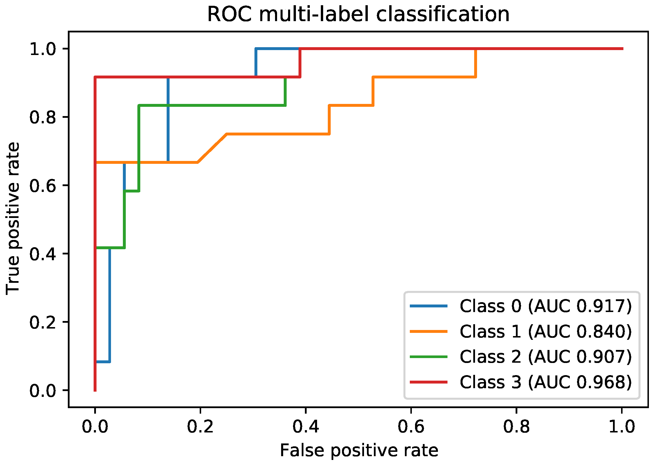
For better measuring the performance of the fine-tuned ensemble, we included ROC curves (receiver operating characteristic) for both binary and multiple-label classification measured on the test set. In the case of multiple-label classification, we used a one versus the rest approach, in which we analyzed each class separately. The analyzed class would have label 1, while all other classes shared label 0. The model could be encouraged to have a higher recall (also known as sensitivity or true positive rate) at the cost of more false positives, or on the contrary, have a lower recall, but also fewer false positives. Our model is not binary in nature; its output is an array with four elements, one for each class. The first step was to run the softmax function over the output to transform it into a four-element array containing probabilities. In the usual case of multiple-label classification, we simply looked at the maximum element from the array to determine the result. However, to calculate the ROC curves, which are suited for binary classification, we analyzed each class in turn versus the rest of the classes. To bias the model in the desired direction (better recall versus less false positives), we looked at two elements from the array of probabilities (which contained four elements): one which corresponded to the analyzed class and the other was its strongest candidate. The strongest candidate was determined by taking the maximum over the other three candidates. We subtracted the probability of the strongest candidate from the probability of the analyzed class and compared it to a threshold. This threshold could take values from one to minus one, corresponding to the extreme cases when the model was certain on the analyzed class and all other candidates had zero probability and to the case when the model was certain on a candidate and all other probabilities were zero. Please note that all four probabilities summed to one because they were computed using the softmax function. The model could be influenced by leveraging the difference between the probabilities of the analyzed class and the best candidate. As noted, this difference could take values in the range [−1, 1]. We compared this difference with a threshold: if the difference was greater than the threshold, we considered outcome one (the analyzed class was detected), otherwise we considered outcome zero (another class was detected). By setting different values to this threshold in the range [−1, 1], we could compute the ROC curve for a certain class; this is illustrated in Figure 6. When we set a smaller threshold (including negative), we encouraged a higher recall, since it would be more likely that the calculated difference would be higher than the threshold, resulting in a positive outcome. Setting the threshold to minus one would make the model always return a positive outcome. On the contrary, if we set a higher threshold, the probability differences would be less likely to be bigger then the threshold, favoring precision and fewer false positives. Setting the threshold to one would make the model always return a negative outcome. If the threshold was zero, then the classification was unchanged.

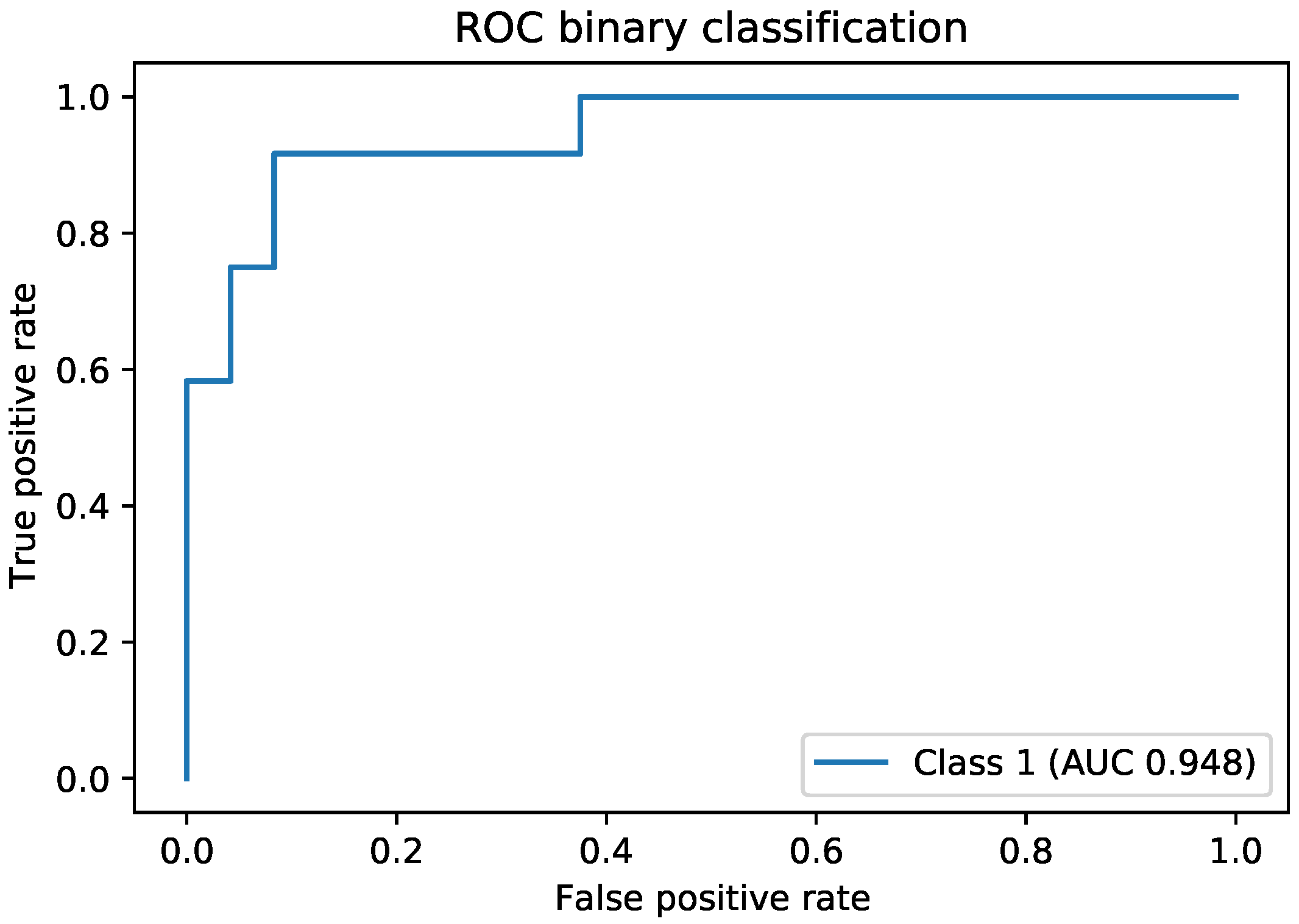
For the binary version of the ensemble, we used a similar approach, with a minor modification. In the binary classification problem, we needed to separate patients with CIN2/3 lesions and cancer from the other less affected patients, with CIN1, and with no lesions. Classes 2 and 3 represented severely affected patients (Outcome 1 in the binary classification problem) and Classes 0 and 1 less affected patients (Outcome 0 in the binary classification problem). In this case, we calculated the difference between the probabilities of the best candidates for Outcome 1 (CIN2/3 and cancer patients) and Outcome 0 (normal and CIN1 patients). In other words, we calculated two maximums corresponding to the two candidates, the maximum of the probabilities of Classes 2 and 3 (best candidate for Outcome 1 in the binary classification problem) and the maximum of the probabilities of Classes 1 and 0 (best candidate for Outcome 0 in the binary classification problem). We subtracted the probabilities of the two best candidates and compared these to a threshold having values in the interval [−1, 1] as before. The ROC curve for the binary classifier is found in Figure 7.

4.3. Time Complexity

We believe that in this domain, the accuracy, recall, and precision of the model are the most important measures. Nevertheless, knowing that sometimes neural networks could be computationally expensive, we measured the execution time of our model to make sure it could be run conveniently on a computer without GPU since we expected that most computers or servers do not own one. At the same time, we compared the time obtained with the other baseline models to emphasize the speedup gained by using the MobileNetV2 [32] architecture. The measurements were performed on Google Colab virtual machines, with two CPU Intel(R) Xeon(R) 2.30 GHz and approximately 12.7 gigabytes of RAM. For measuring the execution speed, we fed to the network a single image at a time since this was the most likely scenario to be found in practice. We calculated the average execution time for each model on the whole test set. The results are displayed in

Table 7. Execution times for the networks’ forward passes.

Model	Execution Time (milliseconds)
ResNeXt-101	904
VGG19	831
DenseNet	233
ResNet18	102
MobileNetV2 (original model)	66
MobileNetV2 (having our modifications)	59
Ensemble	390

. As can be noticed, the ensemble network could process a single input set of seven images in less than half of a second when running on a CPU.

4.4. Handling of Dataset Imbalance

To assess how well a model was balanced, we analyzed the true positive rate per each class. We aimed to create a less biased model; that is, one that did not perform very well on certain classes to the detriment of others. Even though we recorded the per-class true positive rate, we would still like to have a single value that described the ability of the model to be both accurate and balanced. Therefore, we chose to take the harmonic mean of the per-class true positive rate. The harmonic mean penalizes imbalanced models more than the arithmetic mean because lower values in the members of the mean decrease the result of the harmonic mean more than the result of the arithmetic mean. In this section, we describe three series of experiments.

At first, we performed a series of experiments on the images involving acetic acid solution for determining which training procedure yielded the most balanced model for our task. The best results were reported in the case of weighted cross entropy with weights being dynamically recalculated each epoch. The transformation used for the weights calculation was $\varphi \left(x\right)=exp\left(100x\right)$ as described in Section 3.4. The results of this experiment are reported in

Table 8. Results for experiments regarding dataset imbalance. We used the MobileNetV2 tuned model as described in Section 3.2.2 and the images involving an acetic acid solution. TPR stands for true positive rate.

Training Method	Accuracy	Class 0 TPR	Class 1 TPR	Class 2 TPR	Class 3 TPR	TPR Harmonic Mean
Cross entropy loss	71.24%	91.66%	41.66%	65.00%	86.66%	64.69%
Focal loss, $\gamma =1$	67.08%	86.66%	53.33%	55.00%	73.33%	64.40%
Focal loss, $\gamma =2$	66.66%	66.66%	61.66%	56.66%	81.66%	65.45%
Focal loss, $\gamma =5$	66.25%	93.33%	40.00%	56.66%	75.00%	59.97%
Weighted cross entropy, weights fixed to the ratio of each class in the training population	67.08%	91.66%	50.00%	48.33%	78.33%	62.14%
Weighted cross entropy, weights recalculated each epoch, $\varphi \left(x\right)=x^3$	71.66%	83.33%	53.33%	70.00%	80.00%	69.52%
Weighted cross entropy, weights recalculated each epoch, $\varphi \left(x\right)=exp\left(x\right)$	70.41%	86.66%	46.66%	71.66%	76.66%	66.70%
Weighted cross entropy, weights recalculated each epoch, $\varphi \left(x\right)=exp\left(10x\right)$	70.00%	78.33%	55.00%	66.66%	80.00%	68.43%
Weighted cross entropy, weights recalculated each epoch, $\varphi \left(\mathbf{x}\right)=\mathbf{exp}\left(\mathbf{100}\mathbf{x}\right)$	71.25%	80.00%	65.00%	61.66%	78.33%	70.33%

.

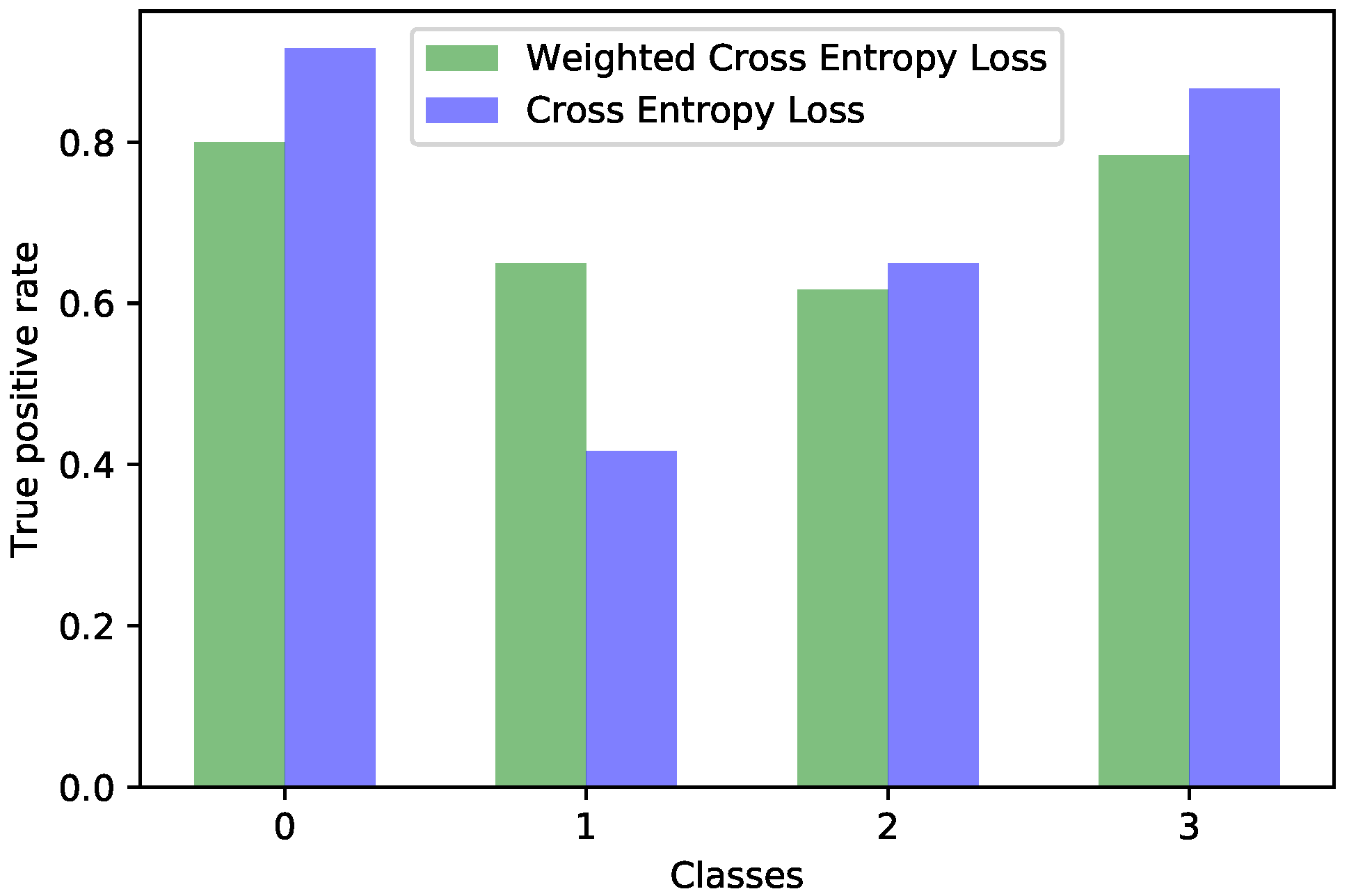
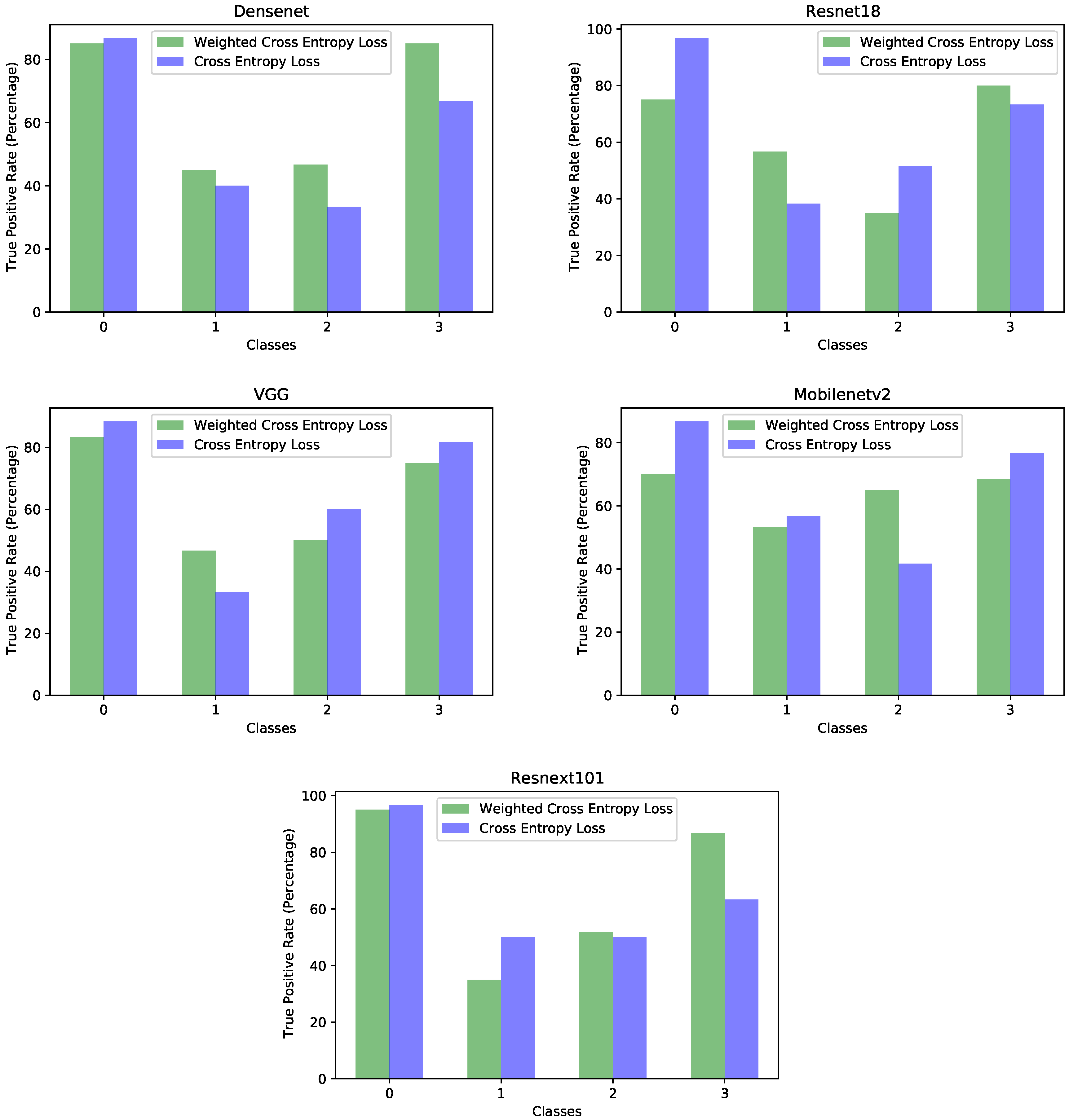
Next, we validated the best performing approach on the other baseline models to see if it brought similar qualities of better balancing the classification bias. As can be observed from the numbers in

Table 9. Results for training using the weighted cross entropy versus simple cross entropy on the baselines models. The transformation applied to the errors is $\varphi \left(x\right)=exp\left(100x\right)$ as explained in Section 3.4, except for VGG, where we applied a transformation of $\varphi \left(x\right)=exp\left(x\right)$. The training of this network did not converge having the other transformation. Some of the models trained with weighted cross entropy record better-balanced true positive rates as measured by the harmonic mean. In the table, TPR stands for true positive rate, WCE stands for weighted cross entropy, and CE stands for cross entropy.

Loss	Model	Image Types	Accuracy	Class 0 TPR	Class 1 TPR	Class 2 TPR	Class 3 TPR	TPR Harmonic Mean
CE	DenseNet	Acetic acid	66.66%	86.66%	40.00%	33.33%	66.66%	49.05%
WCE	DenseNet	Acetic acid	65.41%	85.00%	45.00%	46.66%	85.00%	59.54%
CE	ResNet18	Acetic acid	65.00%	96.66%	38.33%	51.66%	73.33%	57.61%
WCE	ResNet18	Acetic acid	61.66%	75.00%	56.66%	35.00%	80.00%	55.51%
CE	VGG	Acetic acid	65.83%	88.33%	33.33%	60.00%	81.66%	56.95%
WCE	VGG	Acetic acid	63.75%	83.33%	46.66%	50.00%	75.00%	59.91%
CE	MobileNetV2	Acetic acid	65.41%	86.66%	56.66%	41.66%	76.66%	60.39%
WCE	MobileNetV2	Acetic acid	64.16%	70.00%	53.33%	65.00%	68.33%	63.43%
CE	ResNeXt-101	Acetic acid	65.00%	96.66%	50.00%	50.00%	63.33%	60.48%
WCE	ResNeXt-101	Acetic acid	67.08%	95.00%	35.00%	51.66%	86.66%	57.15%

and Figure 8, this method created better balanced models for DenseNet [43], VGG [42], and MobileNetV2 [32], but did not bring any advantage for ResNet18 [37] and ResNeXt-101 [44]. Moreover, for ResNet18, we used a different transform of $\varphi \left(x\right)=exp\left(x\right)$ to make the training converge. These results showed that this method could decrease the classification bias on the imbalanced datasets, but it is not guaranteed to work for every combination of model, dataset, and meta-parameters. In practice, it requires a careful meta-parameter fine-tuning, especially the learning rate and the transformation used for calculating the weights. The idea of the method is to work on the harder problem more, an intuitively correct idea that is not new in machine learning. However, neural networks’ learning is very complex and most often converges to different local minima. In practice, the developer should experiment with more solutions and choose the best working one. The method described in this section could be an important candidate.

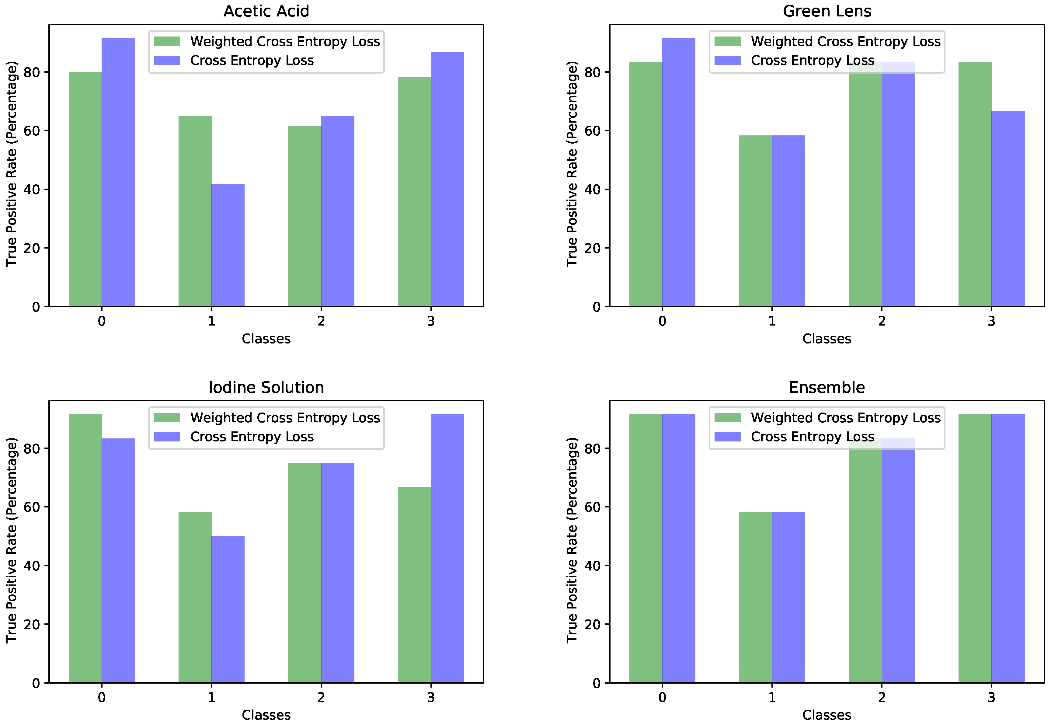
As a next step, we applied this training method to the rest of the images involving the green lens and the iodine solution and finally to the ensemble as a whole. This method proved beneficial for the images with an acetic acid solution and those through the green lens. In the case of those with an acetic acid solution, the overall accuracy did not change much, but the model was better balanced, while in the case of images through the green lens, both overall accuracy and class balance got better. Unfortunately, in the case of iodine solution images, the performance of the model degraded. For this reason, we decided to experiment with an ensemble formed from the models trained with weighted cross entropy for the images with acetic acid and through the green lens, but used the classical training procedure (simple cross entropy) for images with iodine solution. The ensemble convolutional network was trained with weighted cross entropy just like the other networks. We measured the overall accuracy and true positive rate per each class for this ensemble as we did for the single networks. At the same time, we did the same measurement for the ensemble trained classically. The results were surprising; both models displayed the same numbers for overall accuracy and true positive rate per each class. The ensemble made a much better use of the data available, taking advantage of both visual features and the relationships between multiple images. The ensemble adapted to the different image representations and provided the same outcome despite the differences in the image representations provided by the MobileNetV2 networks that were trained in different ways. In our opinion, this stability is an advantage. It can also mean that the image relationships might be more important than the individual image features in the overall performance of the system.

Table 10. Results for training the ensemble and the single networks on the different image types with weighted cross entropy versus simple cross entropy. The transformation applied to the errors is $\varphi \left(x\right)=exp\left(100x\right)$ as explained in Section 3.4. The network trained with weighted cross entropy on iodine solution images is not included in the ensemble trained with weighted cross entropy and is replaced with the one trained with cross entropy because it has a better performance. Both ensembles trained with weighted cross entropy and simple cross entropy share the same accuracy and per-class true positive rates. Please note that in this comparison, we did not fine-tune any of the ensembles. In the table, TPR stands for true positive rate, WCE stands for weighted cross entropy, and CE stands for cross entropy.

Loss	Model	Image Types	Accuracy	Class 0 TPR	Class 1 TPR	Class 2 TPR	Class 3 TPR	TPR Harmonic Mean
CE	MobileNetV2	Acetic acid	71.24%	91.66%	41.66%	65.00%	86.66%	64.69%
WCE	MobileNetV2	Acetic acid	71.25%	80.00%	65.00%	61.66%	78.33%	70.33%
CE	MobileNetV2	Green lens	75.00%	91.66%	58.33%	83.33%	66.66%	72.65%
WCE	MobileNetV2	Green lens	77.08%	83.33%	58.33%	83.33%	83.33%	75.26%
CE	MobileNetV2	Iodine solution	75.00%	83.33%	50.00%	75.00%	91.66%	71.12%
WCE	MobileNetV2	Iodine solution	72.91%	91.66%	58.33%	75.00%	66.66%	70.94%
WCE/CE	Ensemble	All images	81.25%	91.66%	58.33%	83.33%	91.66%	78.49%

displays the results of this experiment. Figure 9 is a visualization of Table 10, each subplot displaying the comparison of the per-class true positive rates for the training on a certain type of image.

4.5. Network Activation Visualization

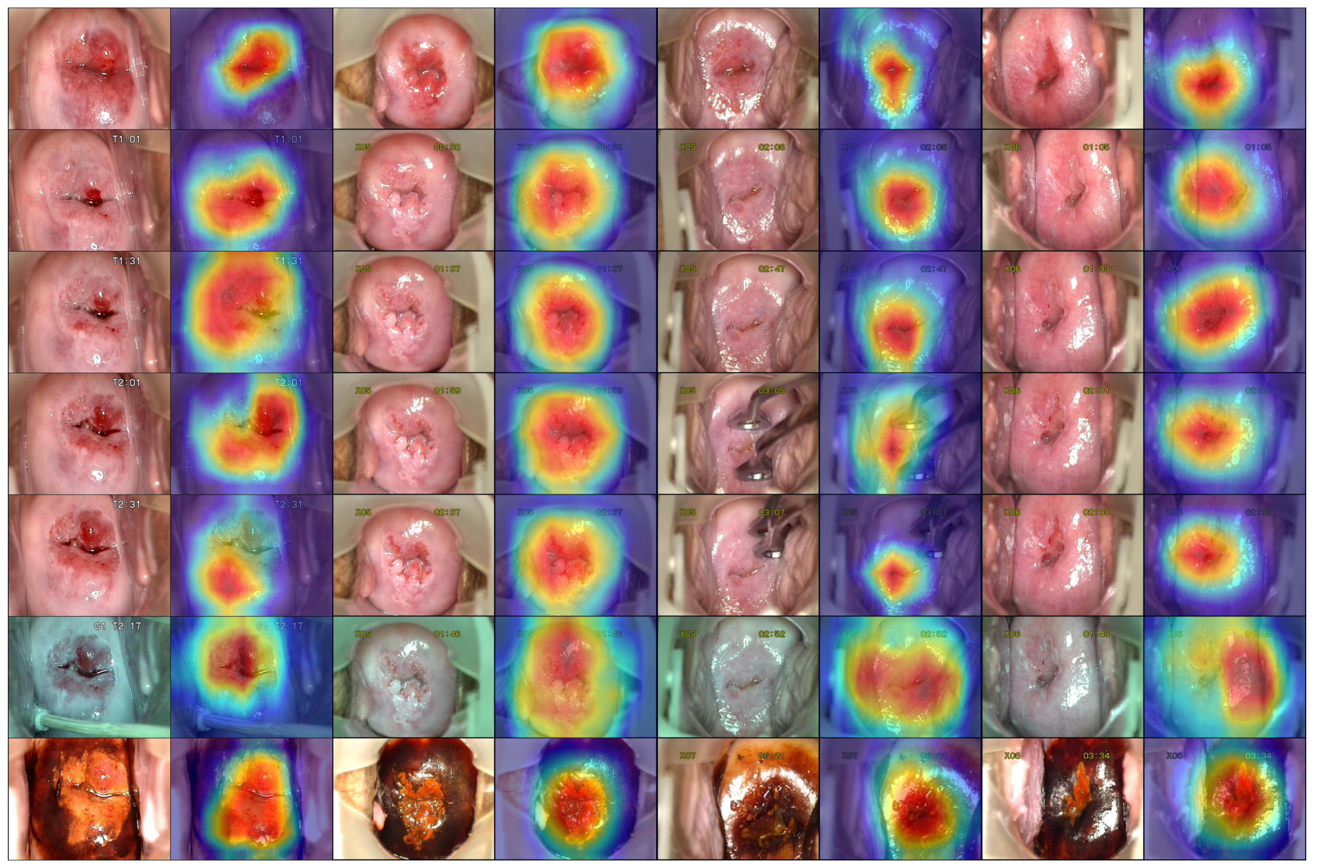
The images from colposcopy contain noise in different forms, such as time displayed by the camera, speculum, vaginal walls, light reflections, and sometimes additional objects such as cotton buds used for cleaning up the cervix. We wanted to find if the network picked those features resulting in overfitting. We used a method named GradCAM++[45] to visualize the areas of the image that triggered the result of the network. GradCAM++ is a generalization over a previous version named GradCAM [46]. In both methods, the mask used for visualization is calculated by multiplying the activations from the forward pass through a chosen network layer with certain weights calculated using the backpropagation of the result through that layer. We applied this visualization technique to our ensemble, which received as input seven images, resulting in seven network activation heat maps. We computed the heat maps based on the last convolutional layer of each of the three networks composing the ensemble. We used the final convolutional layer because choosing deeper layers provided better localization abilities [46]. Therefore, on a single ensemble run, we obtained seven heat maps for the seven images: the first five were calculated on the convolutional network specific to acetic acid images, and the other two heat maps were calculated on the networks relevant to the green lens and iodine solution images. The activation heat maps were a very useful tool to provide clues about model errors and to give ideas for further improvement. From our analysis on the test set, we concluded that the network ignored the text displayed by the camera and was resistant to objects such as cotton buds and other medical devices present sometimes during colposcopy. However, in some cases, it showed problems in distinguishing the cervix area from the vaginal walls and sometimes the speculum walls; it also became distracted by the strong light reflections. However, these adverse effects were only present in a limited number of samples. We believe that increasing the data volume for training could teach the network to better handle these cases. Figure 10 displays selected samples of images and their associated network activations heat maps, these examples present both positive and negative behaviors. Furthermore, the work in [47] details a method for preprocessing the cervigrams by removing the speculum, vaginal walls, and light reflections from the image. This could be a possible enhancement of the system.

4.6. Note on Reproducibility

All of the experiments were implemented in Python, using the PyTorch framework. Even though PyTorch is a great framework for building deep learning software, it has certain limitations with regards to measurement reproducibility. According to the documentation of PyTorch [48], if using different PyTorch releases, commits, or platforms, then the results of the experiments might differ. Additionally, in the documentation [48], it is mentioned that: “results need not be reproducible between CPU and GPU executions, even when using identical seeds”. All of our experiments were carried out in the cloud, either in Google Colab or by renting different GPU units for limited periods. The control of the host was achieved using Jupyter notebooks or the web interface available in Google Colab if using that environment. Therefore, we used a multitude of environments, including virtual machines run in the cloud. Consequently, we can not guarantee that our measurements are reproducible. However, if trying to reproduce, then we expect that the results will not diverge by a large margin. Together with the source code, we included the model checkpoints that resulted from the experiments; those will provide reproducible results provided they are tested in the same way. Eventually, a researcher could make good use of the checkpoints by applying the transfer learning techniques.

5. Discussion

In deep learning, there is an infinite set of variations to be chosen from when it comes to network structure, parameters, and training procedures. For this reason, you might hear from some people that deep learning is like “art”; this expresses the freedom and lack of constraints in designing a solution. We approached this problem with an incremental strategy similar to gradient descent. It was impossible to find the best solution; therefore, we searched for a setup that worked well among a predefined set of experiments, then we explored additional aspects while keeping the tested ones fixed. For choosing the correct set of experiments at each step, the researcher relies on intuition and prior knowledge. In this section, we describe the journey we took for arriving at the final solution and highlight the most important ideas.

We started with a very simplistic approach, which used a single neural network pretrained on ImageNet [40]. As was noted in the results displayed in Table 5, despite the networks being pretrained, the accuracies were low, most models reporting approximately 64% on the test set. Upon analysis of the results, we concluded that the main reason for the low accuracy was overfitting; thus, we chose a model having a lower capacity, MobileNetV2 [32], and applied to it as much regularization as possible. The most important and less intuitive modification was to change the size, in terms of the number of feature maps (channels), of the last convolutional layer. This modification constrained the capacity of the network while preserving the already learned structure from the ImageNet pretraining. Furthermore, as explained in Section 3.2.2, the last convolutional layer of the MobileNetV2 acts as an adapter, transforming the internal representation of the network to the output representation; thus, it makes sense to change this adapter to better fit the required task. Another regularization technique was the two dimensional dropout layer inserted at the end of the convolution. As you can see, even though the MobileNetV2 network had a smaller capacity compared to other deeper networks, it still needed additional regularization to be effective on this task. If the dataset were larger and more diverse, we could decrease the regularization and take advantage of the full capacity of the network or use more complex models such as the ResNext101 [44] model, which provided the highest capacity and was pretrained on the greatest amount of images [44]. Therefore, the aspects related to regularization could change from one scenario to another, but it is useful to have the knowledge or methodology to better regularize a model, depending on the task. This paper presented such an example. Moreover, datasets on specific medical topics can be much more scarce and reduced in volume compared to others. For this reason, it is important to be able to adapt the existing models to specific tasks that are constrained by a lower volume of data. Our tuning of the MobileNetV2 network resulted in an accuracy of approximately 71%.

Once we decided on the MobileNetV2 network using the experiments made on the images having the acetic acid solution, we extended the solution to the rest of the dataset input, the images through the green lens and with the iodine solution. On those types of images, we reported accuracies of 75% for both image types. The increase in accuracy was most probably due to the distinctive features of these types of images. The green lens helped in creating a stronger contrast against the red color of the cervical lesions. Upon the application of the iodine solution, the abnormal areas changed color, becoming yellow or orange, which made a strong contrast with the dark red color of the iodine solution. These types of images were easier to visualize, even for humans.

Up to this point, we explored all the types of images available; however, we did not take advantage of the existing relations between them and of the temporal sequence displayed by the first five images with the acetic acid solution. This was achieved using the ensemble, which provided the best accuracy reported in this paper of 83% for the four-class problem and 91% for binary classification. A very important aspect to note about the design of the ensemble was the use of representation learning. In the ensemble, we did not use the final output of the MobileNetV2 networks; instead, we used an internal network representation that preserved the spatial information and the relevant features for this classification task. We chose as image representation the output of the last convolutional layer from the MobileNetV2 network. This was a tensor of size $7\times 10\times 32$ for acetic acid images and iodine solution images and of size $7\times 10\times 64$ for green lens images. Thus, when constraining the size of the last convolutional layer in the MobileNetV2 layer, we also had in mind the computation of image representations. If the size of the representation was too large, the network might overfit instead of capturing the generic and useful features. The representations of the images were not learned by the ensemble; they were learned in the previous steps when training the single networks. We tried fine-tuning the ensemble as a whole so that the ensemble could adjust the computation of the representations, but the accuracy was lower, probably due to overfitting issues. For analyzing and relating the seven images together, we used an additional convolutional network made out of a single inverted residual unit, whose structure is described in Table 4. An alternative to this is to use a recurrent neural network; this can be the subject of future research. In our case, we chose the convolutional network over the recurrent version because it does not pose the vanishing and exploding gradient problem and because the sizes of the image representations and the sequence length were both small and made the training through a convolutional network feasible.

Another direction of our study was the handling of the dataset imbalance in the context of the current problem. The first step was to analyze the already existing model (trained with classic cross entropy) to assess the effects of this phenomenon. We used the true positive rate recorded per each class as a measure of classification bias. In an ideal scenario, all classes should present a 100% true positive detection rate; however, in practice, the classes having a higher number of samples performed much better than those with a reduced number of samples. This can be noticed by viewing Figure 3 and Figure 4 in parallel. It also meant that the model could perform better if presented with more data. We should also know that sometimes a higher true positive rate for one class could be attributed to biased learning, and while the model tended to better recognize one class, the rest of the classes would have a lower detection rate; this is especially true for classes that are harder to discriminate. Through our experiments, we tried to reduce this classification bias; ideally, the model should classify samples as if there would be an even distribution between the classes. Apart from the cross entropy loss, we experimented with another two standard losses for imbalanced datasets, the weighted cross entropy and focal loss [41]. For the current problem, we obtained the best results with the weighted cross entropy having a dynamic weight calculation based on the training time reported errors per each epoch. The idea of the training algorithm was to work constantly towards recognizing the harder classes. This method levels the classification bias among the classes; however, it does not guarantee keeping the overall accuracy the same. From our experiments, the overall accuracy stayed approximately the same for the acetic acid solution images, increased for the green lens, because it worked on the problem areas, while for the iodine solution, the overall accuracy dropped. Looking at the true positive rate for each class provided a transparent and accurate view on the behavior of the model; nevertheless, comparing the performance of multiple models this way is hard. Which criteria should be used? Are some classes more important than others? What if a model performs very well on most of the classes, but very poorly on a certain one? For our task, we tried to encourage a model that had a good overall accuracy while distributing its classification bias as evenly as possible. Being inspired by the F1 measure score, which computes the harmonic mean between precision and recall, we computed the harmonic mean of the true positive rates of the classes. The harmonic mean penalizes the smaller values more then the arithmetic mean; thus, imbalanced models would get penalized more, but the overall accuracy is also taken into account. We used this measure for evaluating the effectiveness of the tested strategies. After performing these experiments on each type of image separately, we applied them on the ensemble by training each of the composing models with the established strategy and then the ensemble network as well. Unfortunately, this method did not yield any improvement for the ensemble; the true positive rate per each class was the same as those reported by simple training through cross entropy. The most probable explanation is that the ensemble network already made the best out of the available data, and any training variation around the same model was not able to bring additional advantages. Even though the ensemble could not be improved by these methods, we consider that the results obtained on the single networks and the analysis of the model behavior concerning the class imbalance are important pieces of information. Additionally, it is necessary to raise the awareness of the practitioners about these problems and about the traps of measuring the performance of a model in the context of an imbalanced dataset. Most of the time, the practitioner might not even realize that the dataset being used is imbalanced; an investigation to find this needs to be done.

Unfortunately, the method used (dynamically weighted cross entropy based on training time errors) has some disadvantages as well. The most notable one, which we also emphasize in Section 4.4, is that it does not always work. In certain cases, it even makes the training diverge. However, with proper parameter selection, we expect that it provides good results most of the time. Another notable problem is that the parameter selection could be a complicated process, which requires more experiments. To make matters worse, the training time increases greatly for each experiment, because a smaller learning rate and slow progression across more epochs are required for this method to be effective. In this paper, we employed a transformation to the errors $\varphi \left(x\right)=exp\left(100x\right)$, which was specific to this problem; for other cases, the researchers would need to find the appropriate transformation through experimentation. This is both an advantage since it allows for greater flexibility, but can also be seen as a disadvantage, as it is not generic enough. Nevertheless, in our opinion, this method is worth being taken into account when dealing with imbalanced datasets.

The last experiment that we did was for visualizing the network activations. Most often, the models are evaluated by several metrics that describe their performance from different perspectives. However, the network visualization, even though less popular, could be used as a complementary means of network evaluation and understanding. In this case, there are no numbers to quantify the performance. Still, by observing the activations and reasoning about them, we can draw conclusions about the network. One way is to hunt for overfitting factors, for example if we notice that the network is paying attention to image features that should not matter for the classification problem. In our case, the pictures contained certain noise, such as text displayed by the camera and medical devices. At first, we were worried especially about the text displayed by the camera. We considered hiding that text or resizing the pictures in such a way that it disappeared. Fortunately, the network automatically learned that it was not a relevant feature for our problem. We found out about this through the network activations’ visualization. On the other hand, we learned that the model was sometimes distracted by the vaginal walls and the strong light reflections, a phenomenon also described in the paper [47].

6. Conclusions

We proposed a method for analyzing multiple colposcopy images at once and achieved 83% and 91% accuracies in the four-class and binary classification problems. In this paper, we did not design a network architecture that solved a generic problem; instead, we applied the recent technological advances in deep learning to a specific problem and dataset. For arriving at the solutions described, we performed more than 100 experiments, each consisting of training a network. To keep the article readable and avoid getting lost in less important details, we documented only the relevant findings. In our opinion, one of the hardest obstacles encountered was overfitting. It was overcome through very careful design and parameter tuning. While arriving at our solution, we brought the following innovations:

• The comparison of multiple convolutional network models on the current dataset.
• The use of the MobileNetV2 architecture for colposcopy image understanding and the tuning of this architecture for a dataset with a reduced size. We would like to emphasize that this architecture should not be used only in scenarios where execution speed and memory consumption are constrained; it should also be an important candidate whenever there is a need for a light-weight solution, when overfitting is a major concern, and when fast experimentation is required.
• The design of a convolutional ensemble composed of multiple MobileNetV2 networks for taking advantage of different kinds of images available in a colposcopy procedure. The use of representational learning was an important aspect of the ensemble design and training.
• The techniques used for handling the dataset imbalance cannot be considered original; however, their application to this specific dataset and model were.

Apart from the design of the network, the current paper stresses the importance of properly measuring the performance from the perspective of dataset imbalance, an aspect that many times is neglected by researchers. Furthermore, we believe that the use of the network activations’ visualization could complement the usual network evaluation. This could help in targeting the problems of the model.

We will end this paper by highlighting the advantages, disadvantage, and further research directions. The current solution presented the following advantages:

• Resistant to overfitting and well adapted to reduced datasets.
• Can take advantage of different types of images at the same time.
• Fast execution speed and low memory consumption. If this might not be of interest to the end-user, it is important in the experimentation and design phase, allowing performing more experiments and better parameter tuning given that both computational power and time are not unlimited resources.
• Even with the current regularizations in place, the model promises further performance gains if presented with more data, as noted in Section 3.4. Furthermore, if enough data is available, the regularizations can be relaxed to allow learning of more complex features.
• Adaptable, in the sense that additional MobileNetV2 networks could be added or removed from the ensemble to fit a different setting.

The limitations of the proposed solution were:

• Suboptimal if applied to a very large dataset.
• Would not be able to take advantage of a large sequence of images because we used a convolutional network instead of a recurrent one for modeling the ensemble.
• Does not take advantage of multiple image scales.
• Does not provide hints to the user on the location of the cervical lesions in the image, which would have been a very useful feature.
• In our opinion, the reported results were encouraging to further research in this direction; however, there is still considerable room for improvement, and applying the system to the real world is not feasible at this moment.

There are many possibilities for modeling the task of colposcopy image classification, and as variations, one could try to replace the ensemble inverted residual unit with a recurrent network, try out visual attention mechanisms, images at higher resolutions or at multiple scales, and aligning the images when processing more of them. Using unsupervised learning could provide another research direction in which extracted features are compared and clustered. Moreover, segmentation would be very useful for this system, because it would indicate the problematic tissues to the physician. Such features can be used as the subject of further research.

Colposcopy plays a very important role in the prevention of cervical cancer and it has the potential to save human lives. We believe that this procedure would greatly benefit from computer image processing and the deep learning technology. We hope that such practices will have a positive impact on medicine and will be deployed in many production systems soon.

References

1. Ginsburg, O.; Bray, F.; Coleman, M.P.; Vanderpuye, V.; Eniu, A.; Kotha, S.R.; Sarker, M.; Huong, T.T.; Allemani, C.; Dvaladze, A.; et al. The global burden of women’s cancers: A grand challenge in global health. Lancet 2017, 389, 847–860. [Google Scholar] [CrossRef]
2. Singh, G.K.; Azuine, R.E.; Siahpush, M. Global Inequalities in Cervical Cancer Incidence and Mortality are Linked to Deprivation, Low Socioeconomic Status, and Human Development. Int. J. MCH AIDS 2012, 1, 17–30. [Google Scholar] [CrossRef] [PubMed]
3. Dereje, N.; Addissie, A.; Worku, A.; Assefa, M.; Abraha, A.; Tigeneh, W.; Kantelhardt, E.J.; Jemal, A. Extent and Predictors of Delays in Diagnosis of Cervical Cancer in Addis Ababa, Ethiopia: A Population-Based Prospective Study. JCO Glob. Oncol. 2020, 6, 277–284. [Google Scholar] [CrossRef] [PubMed]
4. Siegel, R.L.; Miller, K.D.; Jemal, A. Cancer statistics, 2020. CA. Cancer J. Clin. 2020, 70, 7–30. [Google Scholar] [CrossRef]
5. McAlpine, J.N.; Temkin, S.M.; Mackay, H.J. Endometrial cancer: Not your grandmother’s cancer. Cancer 2016, 122, 2787–2798. [Google Scholar] [CrossRef]
6. Fiorica, J.V. The role of topotecan in the treatment of advanced cervical cancer. Gynecol. Oncol. 2003, 90, S16–S21. [Google Scholar] [CrossRef]
7. Janicek, M.F.; Averette, H.E. Cervical Cancer: Prevention, Diagnosis, and Therapeutics. CA. Cancer J. Clin. 2001, 51, 92–114. [Google Scholar] [CrossRef]
8. Saslow, D.; Solomon, D.; Lawson, H.W.; Killackey, M.; Kulasingam, S.L.; Cain, J.; Garcia, F.A.R.; Moriarty, A.T.; Waxman, A.G.; Wilbur, D.C.; et al. American Cancer Society, American Society for Colposcopy and Cervical Pathology, and American Society for Clinical Pathology screening guidelines for the prevention and early detection of cervical cancer. CA Cancer J. Clin. 2012, 62, 147–172. [Google Scholar] [CrossRef] [Green Version]
9. Thomsen, L.T.; Kjær, S.K.; Munk, C.; Frederiksen, K.; Ørnskov, D.; Waldstrøm, M. Clinical Performance of Human Papillomavirus (HPV) Testing versus Cytology for Cervical Cancer Screening: Results of a Large Danish Implementation Study. Clin. Epidemiol. 2020, 12, 203–213. [Google Scholar] [CrossRef] [Green Version]
10. Purwoto, G.; Dianika, H.D.; Putra, A.; Purbadi, S.; Nuranna, L. Modified Cervicography and Visual Inspection With Acetic Acid as an Alternative Screening Method for Cervical Precancerous Lesions. J. Cancer Prev. 2017, 22, 254–259. [Google Scholar] [CrossRef] [Green Version]
11. Soloman, D. The 1988 Bethesda system for reporting cervical/vaginal cytologic diagnoses: Developed and approved at the national cancer institute workshop in Bethesda, MD, December 12–13, 1988. Diagn. Cytopathol. 1989, 5, 331–334. [Google Scholar] [CrossRef] [PubMed]
12. Melnikow, J.; Nuovo, J.; Willan, A.R.; Chan, B.K.; Howell, L.P. Natural history of cervical squamous intraepithelial lesions: A meta- analysis. Obstet. Gynecol. 1998, 92, 727–735. [Google Scholar] [CrossRef] [PubMed]
13. Darragh, T.M.; Colgan, T.J.; Thomas Cox, J.; Heller, D.S.; Henry, M.R.; Luff, R.D.; McCalmont, T.; Nayar, R.; Palefsky, J.M.; Stoler, M.H.; et al. The lower anogenital squamous terminology standardization project for HPV-associated lesions: Background and consensus recommendations from the college of American pathologists and the American society for colposcopy and cervical pathology. Int. J. Gynecol. Pathol. 2013, 32, 76–115. [Google Scholar] [CrossRef] [PubMed] [Green Version]
14. Ji, Q.; Engel, J.; Craine, E. Classifying cervix tissue patterns with texture analysis. Pattern Recognit. 2000, 33, 1561–1573. [Google Scholar] [CrossRef]
15. Balas, C. A novel optical imaging method for the early detection, quantitative grading, and mapping of cancerous and precancerous lesions of cervix. IEEE Trans. Biomed. Eng. 2001, 48, 96–104. [Google Scholar] [CrossRef]
16. Lange, H.; Ferris, D.G. Computer-aided-diagnosis (CAD) for colposcopy. In Proceedings of the Medical Imaging 2005: Image Processing, San Diego, CA, USA, 29 April 2005; Fitzpatrick, J.M., Reinhardt, J.M., Eds.; SPIE: Bellingham, WA, USA, 2005; Volume 5747, p. 71. [Google Scholar] [CrossRef]
17. Srinivasan, Y.; Corona, E.; Nutter, B.; Mitra, S.; Bhattacharya, S. A unified model-based image analysis framework for automated detection of precancerous lesions in digitized uterine cervix images. IEEE J. Sel. Top. Signal Process. 2009, 3, 101–111. [Google Scholar] [CrossRef]
18. Trivizakis, E.; Manikis, G.C.; Nikiforaki, K.; Drevelegas, K.; Constantinides, M.; Drevelegas, A.; Marias, K. Extending 2-D Convolutional Neural Networks to 3-D for Advancing Deep Learning Cancer Classification with Application to MRI Liver Tumor Differentiation. IEEE J. Biomed. Heal. Inform. 2019, 23, 923–930. [Google Scholar] [CrossRef]
19. Whitney, H.M.; Li, H.; Ji, Y.; Liu, P.; Giger, M.L. Comparison of Breast MRI Tumor Classification Using Human-Engineered Radiomics, Transfer Learning from Deep Convolutional Neural Networks, and Fusion Method. Proc. IEEE 2020, 108, 163–177. [Google Scholar] [CrossRef]
20. Tan, T.; Li, Z.; Liu, H.; Zanjani, F.G.; Ouyang, Q.; Tang, Y.; Hu, Z.; Li, Q. Optimize Transfer Learning for Lung Diseases in Bronchoscopy Using a New Concept: Sequential Fine-Tuning. IEEE J. Transl. Eng. Heal. Med. 2018, 6, 1–8. [Google Scholar] [CrossRef]
21. January 2020 Special Issue: Biomedical Imaging and Analysis in the Age of Big Data and Deep Learning|Proceedings of the IEEE. Available online: https://proceedingsoftheieee.ieee.org/view-recent-issues/january-2020/ (accessed on 2 March 2020).
22. Litjens, G.; Kooi, T.; Bejnordi, B.E.; Setio, A.A.A.; Ciompi, F.; Ghafoorian, M.; van der Laak, J.A.; van Ginneken, B.; Sánchez, C.I. A survey on deep learning in medical image analysis. Med. Image Anal. 2017, 42, 60–88. [Google Scholar] [CrossRef] [Green Version]
23. Xu, T.; Zhang, H.; Huang, X.; Zhang, S.; Metaxas, D.N. Multimodal Deep Learning for Cervical Dysplasia Diagnosis. In Proceedings of the Medical Image Computing and Computer-Assisted Intervention—MICCAI 2016, Athens, Greece, 17–21 October 2016; Ourselin, S., Joskowicz, L., Sabuncu, M.R., Unal, G., Wells, W., Eds.; Springer International Publishing: Cham, Switzerland, 2016; pp. 115–123. [Google Scholar] [CrossRef]
24. Almubarak, H.A.; Stanley, R.J.; Long, R.; Antani, S.; Thoma, G.; Zuna, R.; Frazier, S.R. Convolutional Neural Network Based Localized Classification of Uterine Cervical Cancer Digital Histology Images. In Proceedings of the Procedia Computer Science, Chicago, IL, USA, 1 November 2017; Elsevier B.V.: Amsterdam, The Netherlands, 2017; Volume 114, pp. 281–287. [Google Scholar] [CrossRef]
25. Sato, M.; Horie, K.; Hara, A.; Miyamoto, Y.; Kurihara, K.; Tomio, K.; Yokota, H. Application of deep learning to the classification of images from colposcopy. Oncol. Lett. 2018, 15, 3518–3523. [Google Scholar] [CrossRef] [PubMed] [Green Version]
26. Miyagi, Y.; Takehara, K.; Miyake, T. Application of deep learning to the classification of uterine cervical squamous epithelial lesion from colposcopy images. Mol. Clin. Oncol. 2019, 11, 583–589. [Google Scholar] [CrossRef] [PubMed]
27. Monsur, S.A.; Adeshina, S.A.; Sud, S.; Soboyejo, W.O. A mobile-based image analysis system for cervical cancer detection. In Proceedings of the 2017 13th International Conference on Electronics, Computer and Computation (ICECCO), Abuja, Nigeria, 28–29 November 2017; Institute of Electrical and Electronics Engineers Inc.: Piscataway, NJ, USA, 2018; pp. 1–5. [Google Scholar] [CrossRef]
28. Lin, H.; Hu, Y.; Chen, S.; Yao, J.; Zhang, L. Fine-grained classification of cervical cells using morphological and appearance based convolutional neural networks. IEEE Access 2019, 7, 71541–71549. [Google Scholar] [CrossRef]
29. Zhang, T.; Luo, Y.M.; Li, P.; Liu, P.Z.; Du, Y.Z.; Sun, P.; Dong, B.; Xue, H. Cervical precancerous lesions classification using pre-trained densely connected convolutional networks with colposcopy images. Biomed. Signal Process. Control. 2020, 55, 101566. [Google Scholar] [CrossRef]
30. Xu, T.; Xin, C.; Long, L.R.; Antani, S.; Xue, Z.; Kim, E.; Huang, X. A New Image Data Set and Benchmark for Cervical Dysplasia Classification Evaluation. In Proceedings of the Machine Learning in Medical Imaging, Munich, Germany, 5 October 2015; Springer International Publishing: Berlin/Heidelberg, Germany, 2015; pp. 26–35. [Google Scholar] [CrossRef]
31. Chen, H.; Yang, L.; Li, L.; Li, M.; Chen, Z. An efficient cervical disease diagnosis approach using segmented images and cytology reporting. Cogn. Syst. Res. 2019, 58, 265–277. [Google Scholar] [CrossRef]
32. Sandler, M.; Howard, A.; Zhu, M.; Zhmoginov, A.; Chen, L.C. MobileNetV2: Inverted Residuals and Linear Bottlenecks. In Proceedings of the IEEE Conference on Computer Vision and Pattern Recognition (CVPR), Salt Lake City, UT, USA, 18–23 June 2018; pp. 4510–4520. [Google Scholar]
33. Yue, Z.; Ding, S.; Zhao, W.; Ma, J. Cervigram Image Dataset. Available online: http://dx.doi.org/10.21227/bbc5-a202 (accessed on 24 December 2019).
34. Howard, A.G.; Zhu, M.; Chen, B.; Kalenichenko, D.; Wang, W.; Weyand, T.; Andreetto, M.; Adam, H. MobileNets: Efficient Convolutional Neural Networks for Mobile Vision Applications. arXiv 2017, arXiv:1704.04861. [Google Scholar]
35. Chollet, F. Xception: Deep Learning with Depthwise Separable Convolutions. In Proceedings of the 2017 IEEE Conference on Computer Vision and Pattern Recognition (CVPR), Honolulu, HI, USA, 21–26 July 2017. [Google Scholar]
36. Zhang, X.; Zhou, X.; Lin, M.; Sun, J. ShuffleNet: An Extremely Efficient Convolutional Neural Network for Mobile Devices. arXiv 2017, arXiv:1707.01083. [Google Scholar]
37. He, K.; Zhang, X.; Ren, S.; Sun, J. Deep Residual Learning for Image Recognition. In Proceedings of the 2016 IEEE Conference on Computer Vision and Pattern Recognition (CVPR), Las Vegas, NV, USA, 27–30 June 2016; pp. 770–778. [Google Scholar]
38. MOBILENET V2. Available online: https://pytorch.org/hub/pytorch_vision_mobilenet_v2/ (accessed on 27 April 2020).
39. vision/mobilenet.py at master · pytorch/vision · GitHub. Available online: https://github.com/pytorch/vision/blob/master/torchvision/models/mobilenet.py (accessed on 28 April 2020).
40. Russakovsky, O.; Deng, J.; Su, H.; Krause, J.; Satheesh, S.; Ma, S.; Huang, Z.; Karpathy, A.; Khosla, A.; Bernstein, M.; et al. ImageNet Large Scale Visual Recognition Challenge. Int. J. Comput. Vis. (IJCV) 2015, 115, 211–252. [Google Scholar] [CrossRef] [Green Version]
41. Lin, T.; Goyal, P.; Girshick, R.B.; He, K.; Dollár, P. Focal Loss for Dense Object Detection. arXiv 2017, arXiv:1708.02002. [Google Scholar]
42. Simonyan, K.; Zisserman, A. Very Deep Convolutional Networks for Large-Scale Image Recognition. arXiv 2014, arXiv:1409.1556. [Google Scholar]
43. Huang, G.; Liu, Z.; Van Der Maaten, L.; Weinberger, K.Q. Densely Connected Convolutional Networks. In Proceedings of the 2017 IEEE Conference on Computer Vision and Pattern Recognition (CVPR), Honolulu, HI, USA, 21–26 July 2017. [Google Scholar]
44. Mahajan, D.; Girshick, R.; Ramanathan, V.; He, K.; Paluri, M.; Li, Y.; Bharambe, A.; van der Maaten, L. Exploring the Limits of Weakly Supervised Pretraining. In Proceedings of the European Conference on Computer Vision (ECCV), Munich, Germany, 8–14 September 2018. [Google Scholar]
45. Chattopadhay, A.; Sarkar, A.; Howlader, P.; Balasubramanian, V.N. Grad-CAM++: Generalized Gradient-Based Visual Explanations for Deep Convolutional Networks. In Proceedings of the 2018 IEEE Winter Conference on Applications of Computer Vision (WACV), Lake Tahoe, NV, USA, 12–15 March 2018; pp. 839–847. [Google Scholar] [CrossRef] [Green Version]
46. Selvaraju, R.R.; Cogswell, M.; Das, A.; Vedantam, R.; Parikh, D.; Batra, D. Grad-CAM: Visual Explanations from Deep Networks via Gradient-Based Localization. In Proceedings of the 2017 IEEE International Conference on Computer Vision (ICCV), Venice, Italy, 22–29 October 2017; pp. 618–626. [Google Scholar]
47. Das, A.; Kar, A.; Bhattacharyya, D. Preprocessing for Automating Early Detection of Cervical Cancer. In Proceedings of the 2011 15th International Conference on Information Visualisation, London, UK, 13–15 July 2011; pp. 597–600. [Google Scholar]
48. PyTorch. (version 1.4.0). Available online: https://pytorch.org/docs/stable/notes/randomness.html (accessed on 15 February 2020).
Figure 1. Dataset sample: the first five images correspond to the application of the acetic acid solution; the image from the penultimate column is viewed through a green lens; and the image in the last column displays the application of iodine solution. The sample corresponds to Class 2 (Cervical Intraepithelial Neoplasia 2/3). In the images, it can be observed how the area below the cervix opening turns whiter after the application of the acetic acid solution.
Processes 08 00595 g001
Figure 2. Forward pass through the ensemble.
Processes 08 00595 g002
Figure 3. The training data contain 51.28%, 15.61%, 28.43%, and 4.66% samples of each class, corresponding to 1540, 469, 854, and 140 images.
Processes 08 00595 g003
Figure 4. True positive rate (recall) for each class for the validation set: 91.66%, 41.66%, 65%, and 86.66%.
Processes 08 00595 g004
Figure 5. True positive rate comparison between the model trained with weighted cross entropy loss and simple cross entropy loss. Only images with acetic acid were used. The class weighting was recalculated in each epoch according to the model error (one minus true positive rate), and we applied a transformation ϕ ( x ) = e x p ( 100 x ) . As can be observed, the model trained with class weighting provided better balanced true positive rates.
Processes 08 00595 g005
Figure 6. ROC curves for the multiple label classification for the fine-tuned ensemble. Each curve is calculated using a one versus the rest approach.
Processes 08 00595 g006
Figure 7. ROC curve for the binary classification for the fine-tuned ensemble.
Processes 08 00595 g007
Figure 8. Per-class true positive rate comparison between models trained with cross entropy and with weighted cross entropy. Each plot displays the result for a different model. These plots are a visualization of the data from Table 9, and the same training procedures and models are used.
Processes 08 00595 g008
Figure 9. Per-class true positive rate comparison between models trained with cross entropy and with weighted cross entropy. Each plot displays the result for a different type of image, except for the ensemble, which takes advantage of all image types at once. These plots are a visualization of the data from Table 10, and the same training procedures and models are used.
Processes 08 00595 g009
Figure 10. The network activations computed with GradCAM++[45] on the last convolutional layer of each network composing the ensemble. We partitioned this image into four columns, each containing the input of a single ensemble run and the corresponding activation heat maps. As can be noted, most of the time, the system looks at the relevant portions of the image, disregarding the noise. It does not pick up the text displayed by the camera, and it also does not take into account the cotton bud, nor the medical device displayed in Columns 1 and 3. In Columns 3 and 4, on the green lens images, the system gets distracted by the vaginal walls and by the light reflections, which could have a negative impact; even so, the majority of the images seem to be robust to these problems. The image was created by the authors from the dataset samples available at [33]. The source code presented in the Supplementary Materials covers the functionality for creating such visualizations.
Processes 08 00595 g010