New Model-Based Analysis Method with Multiple Constraints for Integrated Modular Avionics Dynamic Reconfiguration Process


Abstract
1. Introduction
2. Background
2.1. IMA
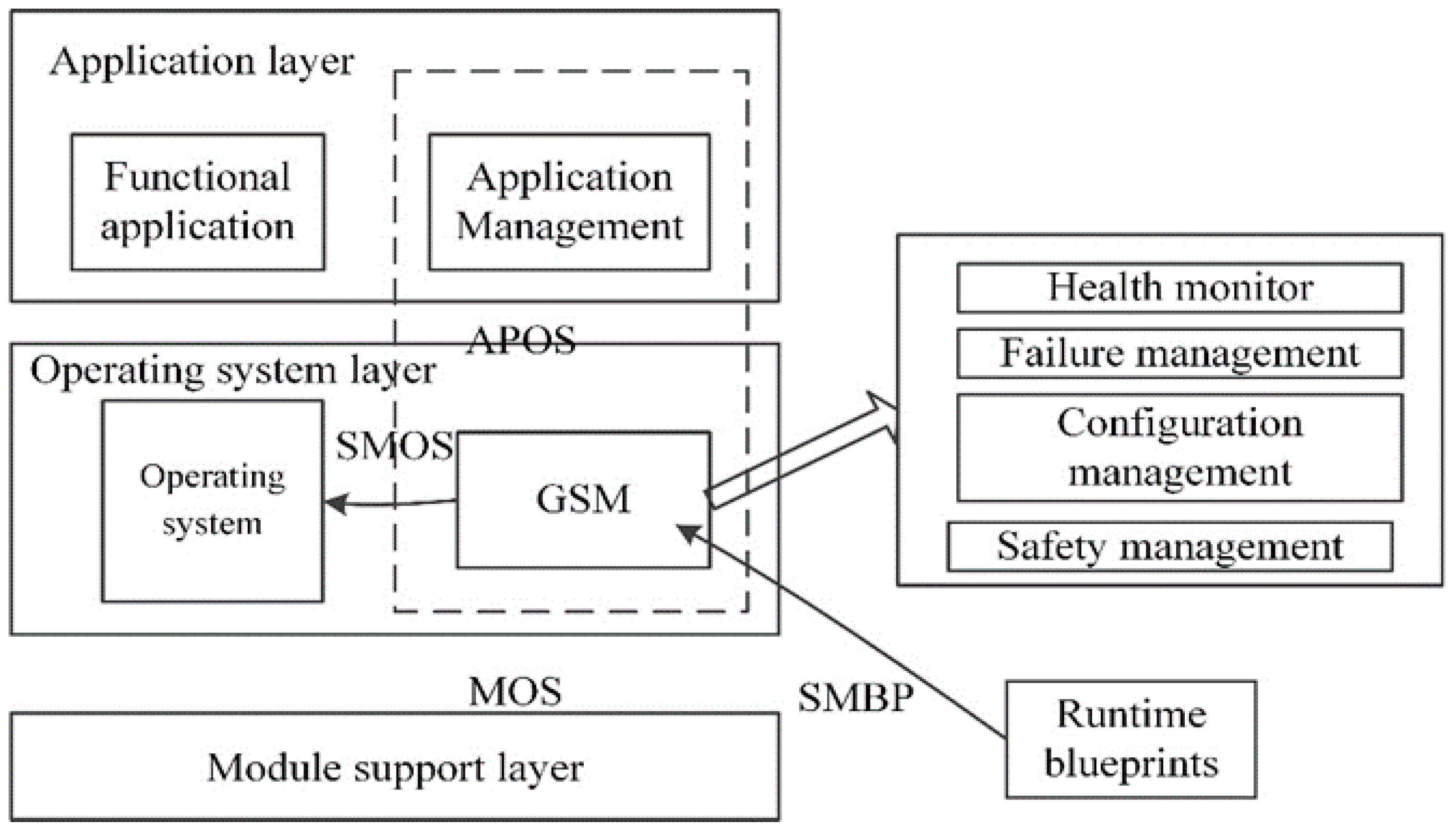
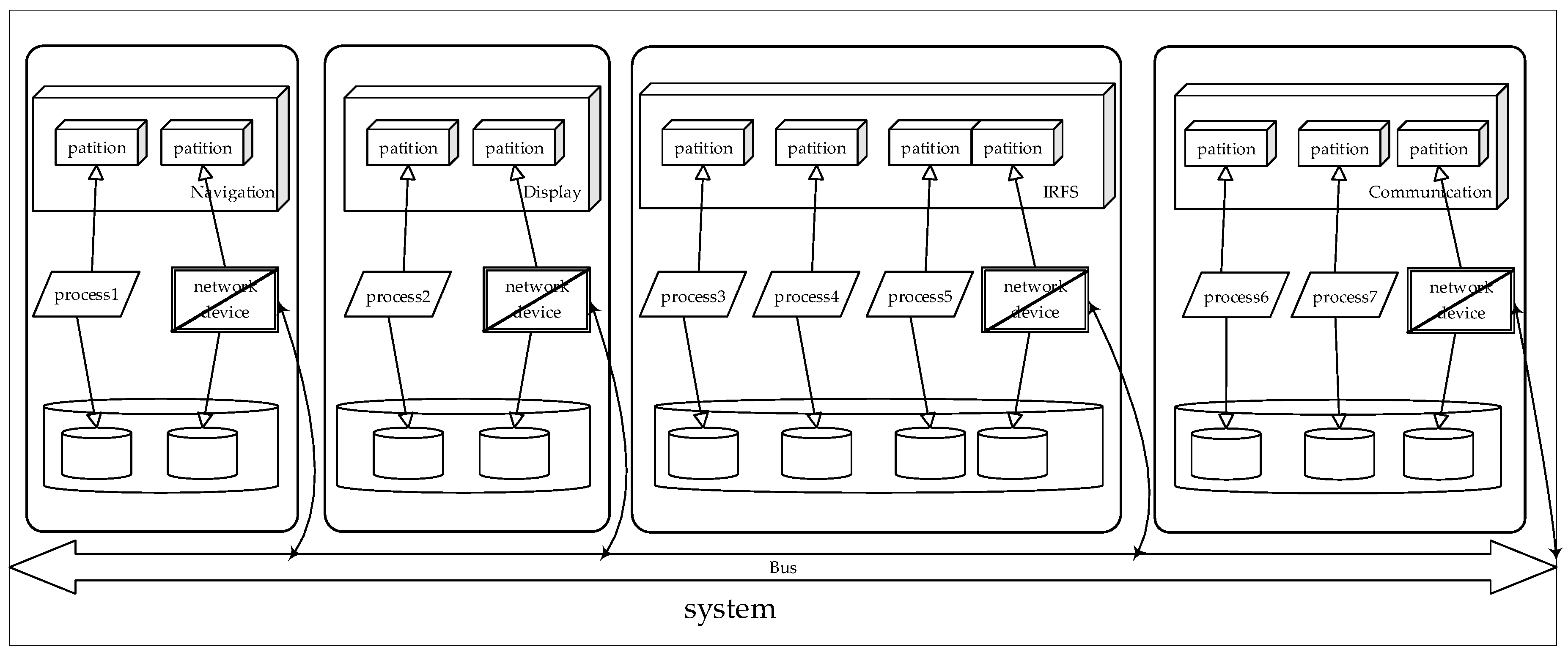
2.1.1. IMA Software Architecture
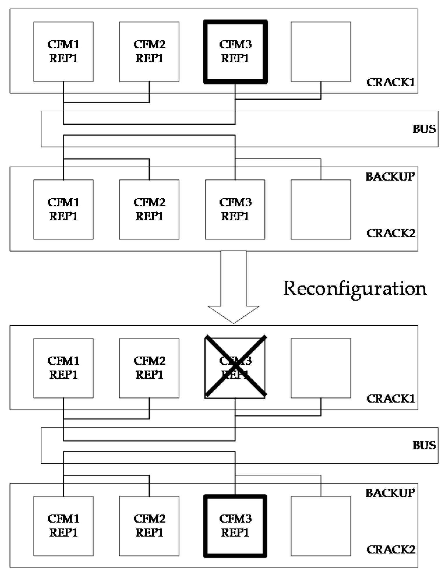
2.1.2. IMA Reconfiguration Mechanism
2.1.3. Related Work for Dynamic Reconfiguration
2.2. AADL
2.2.1. Components
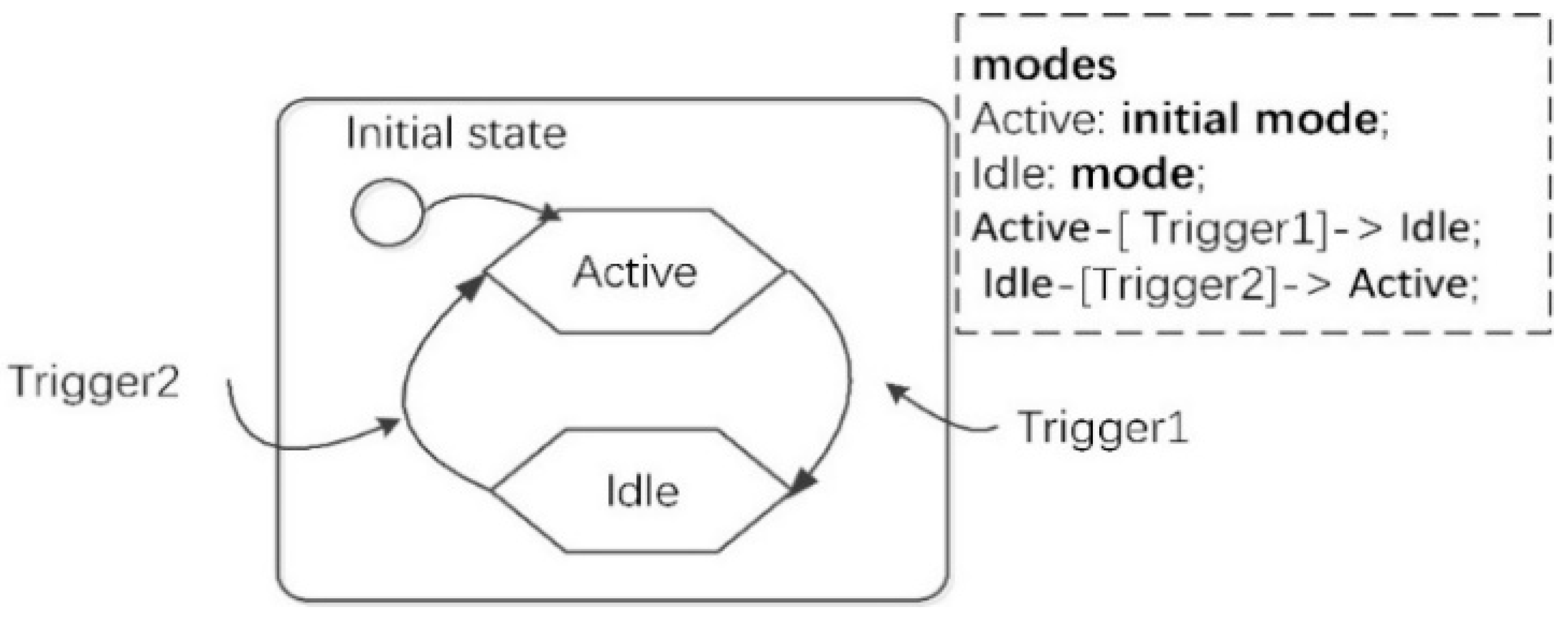
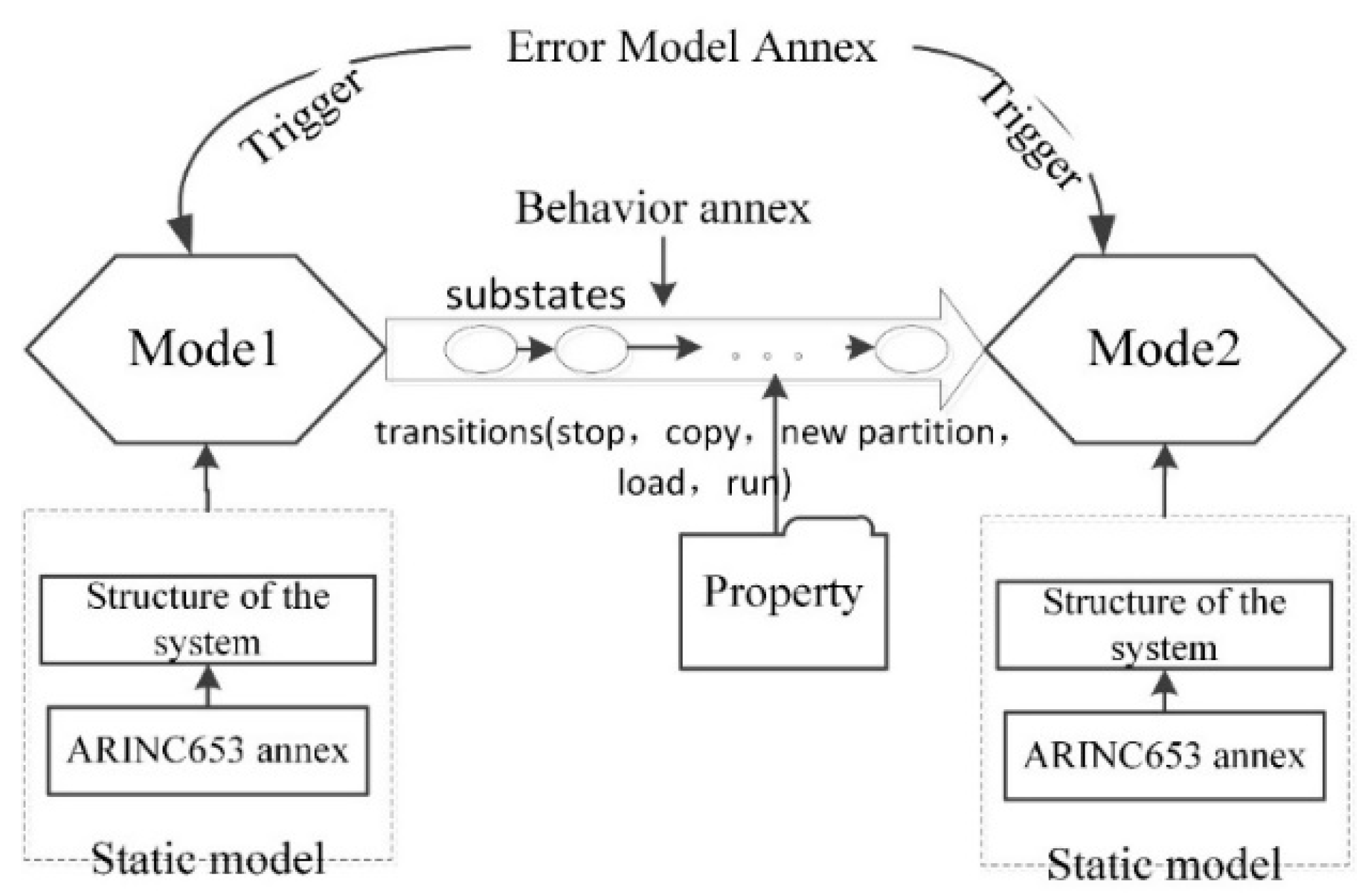
2.2.2. Modes
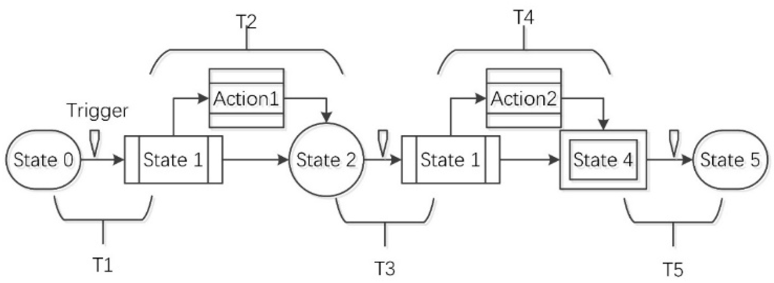
2.2.3. Behavior Annex
2.3. Petri Net
3. Multi-Constraints for the Dynamic Reconfiguration Process
3.1. System State Constraints for Dynamic Reconfiguration
3.2. Real-Time Constraints for System State Transition
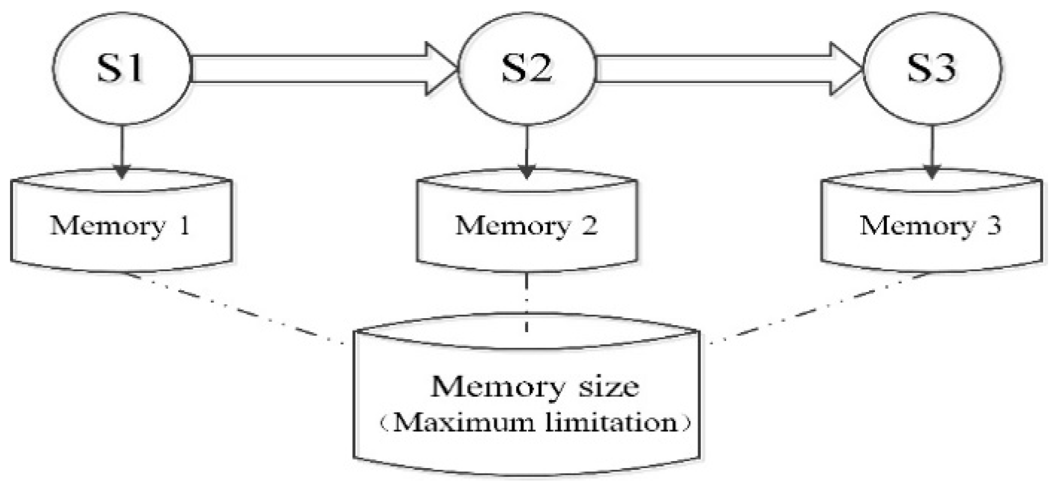
3.3. Memory Constraints for System State
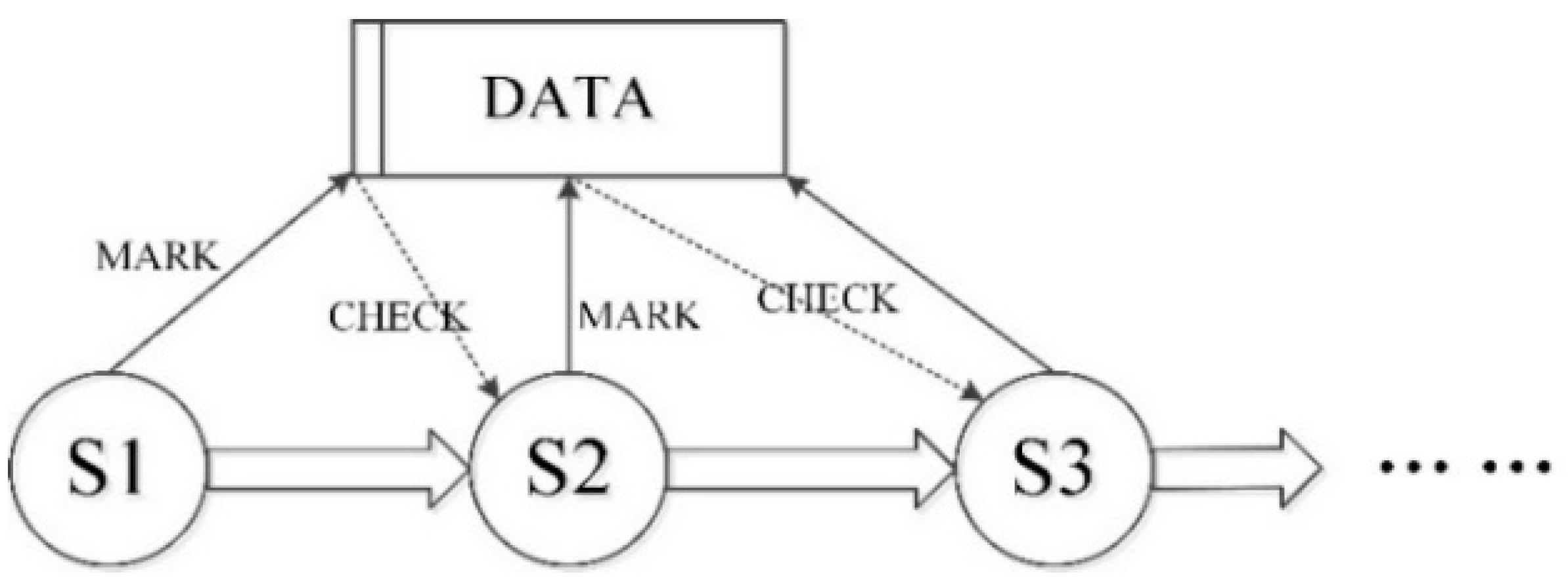
3.4. Ability Constraint for Sharing Data Resources
4. Model-Based Analysis Method
4.1. Modeling Approach Based on AADL
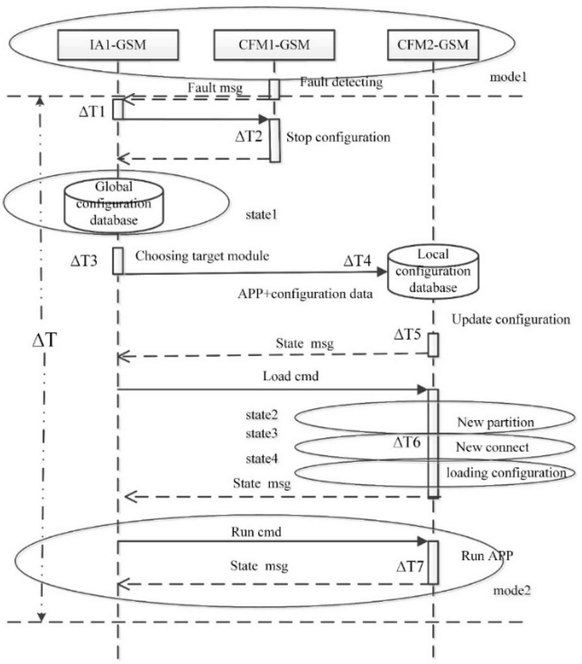
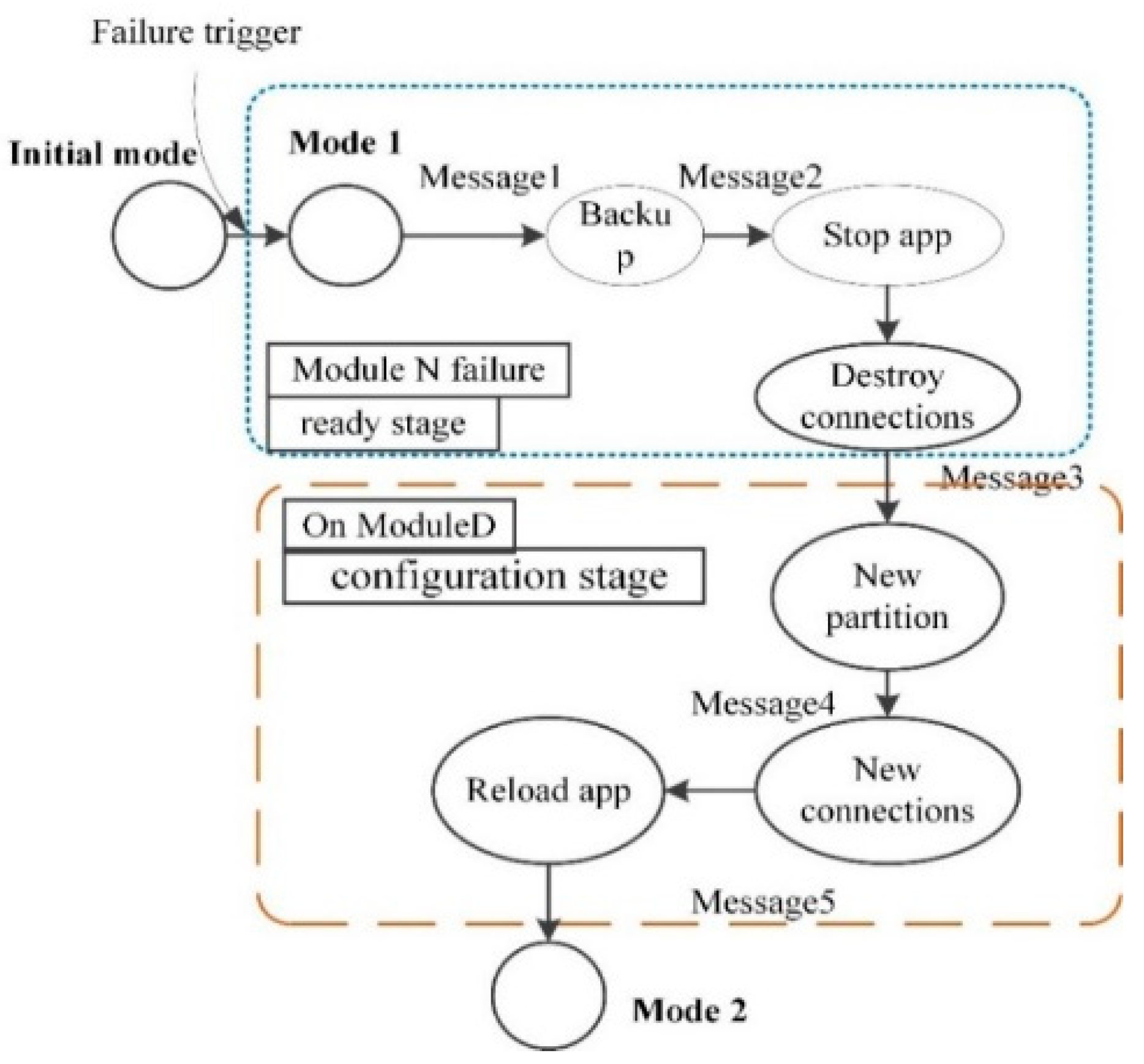
4.1.1. Dynamic Reconfiguration Process
4.1.2. Modeling of the Dynamic Reconfiguration Process
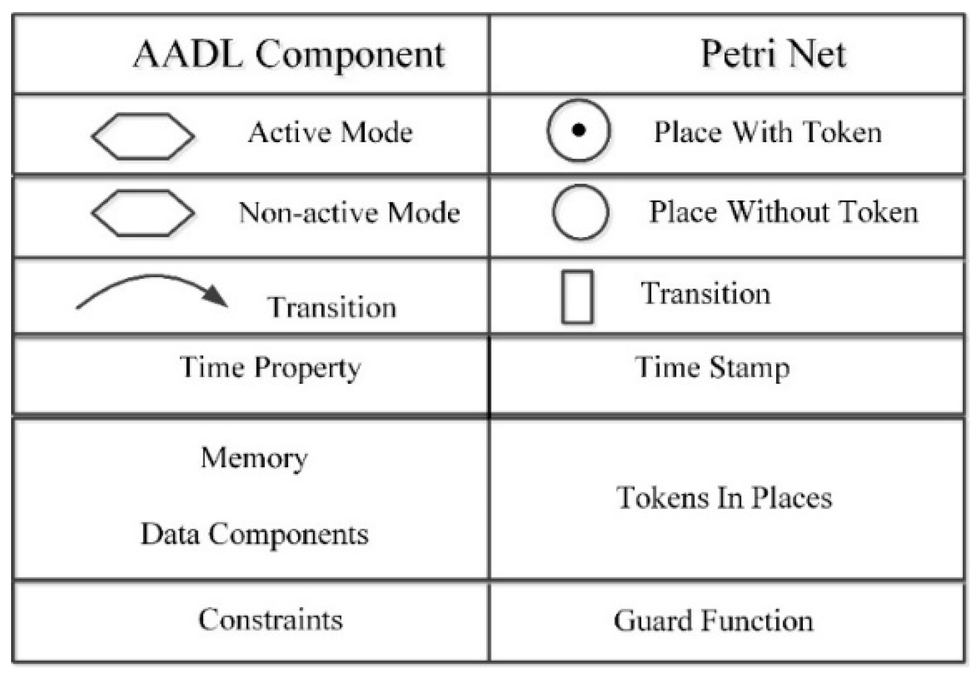
4.2. Rules of Model Transformation
4.3. Simulation Analysis with CPN
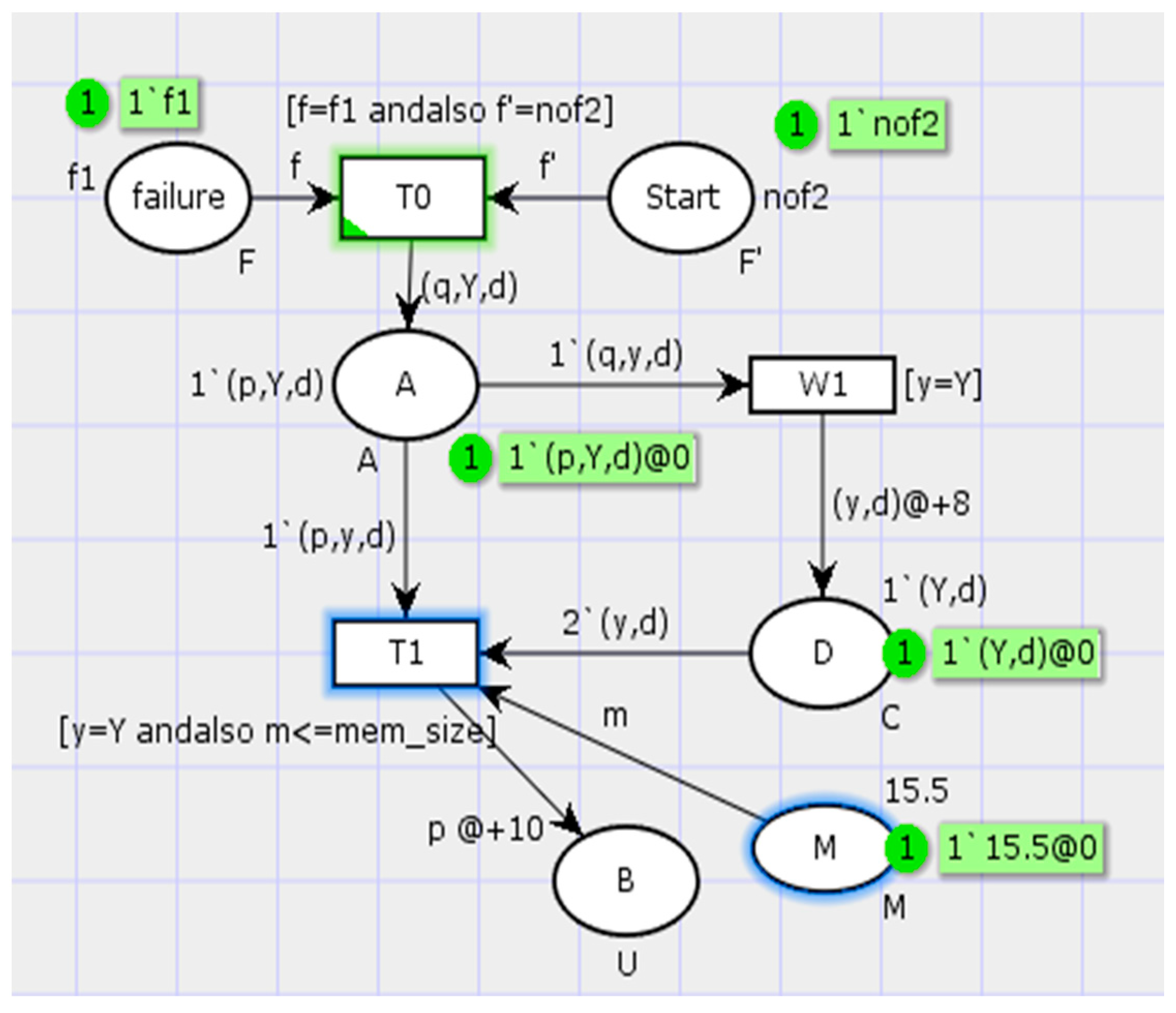
- If all the constraints are fulfilled, the net is simulated to the last place and stops.
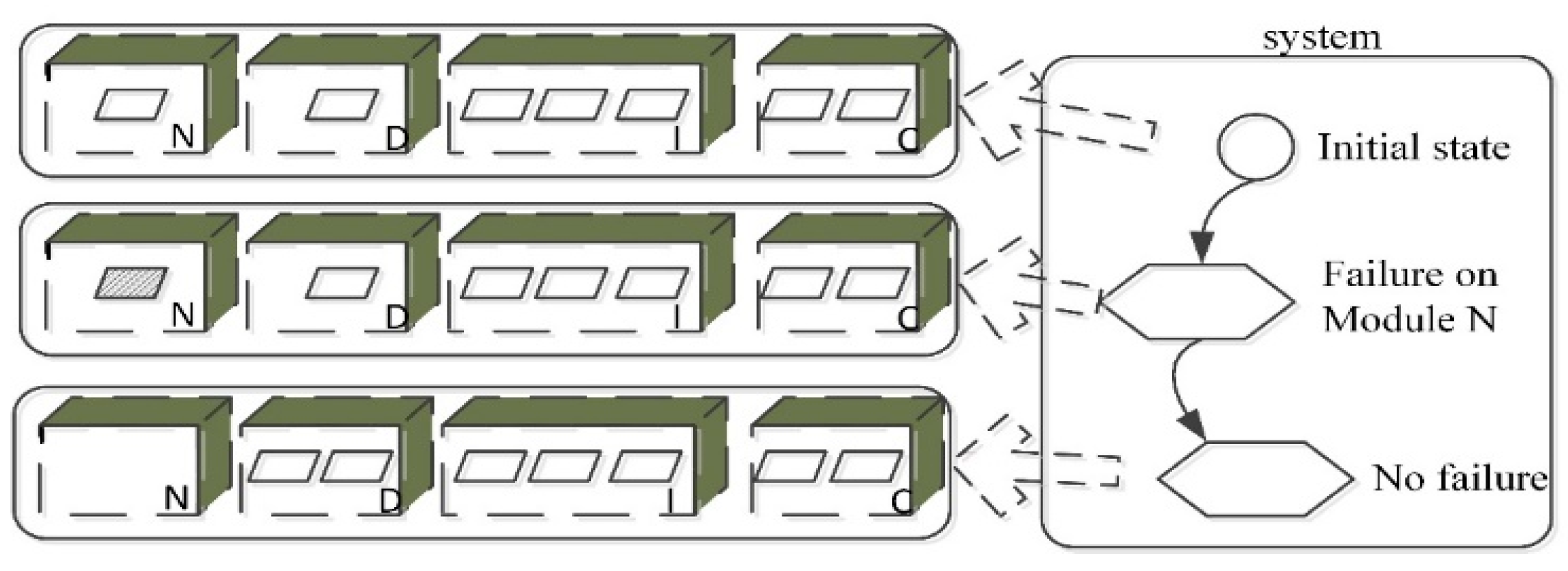
- The system state for dynamic reconfiguration needs checking. The transition T0 can be fired only if the guard function [f = f1 and f’ = nof2] is satisfied. This implies that the failure event occurred for triggering dynamic reconfiguration and did not spread to affect the other modules of the system.
- It should be determined whether the real-time constraints of the system state transition are satisfied or not. Every step in the simulation process is recorded by the time stamp in the transition. When one is step completed, the time consumed is compared with the real-time constraints. The result can tell us if the real-time constraints are met. There is a weakness in this constraint, in that the simulation must be operated manually step by step.
- Memory constraints of system state do not meet the requirements. A guard function of T1 [y = Y and m ≤ mem_size] is set to define whether the memory size occupied in a state (the color set M) is less than the memory size limitation. In this net, the memory size limitation is 10 M, whereas 15.5 M is required in the process. Then, the net simulation ceases at T1 because it cannot be fired without meeting the guard function.
- The ability constraint for sharing data resources is fulfilled. If the token from place A to transition W1 does not meet the guard function, the simulation stops. In this net, Y in color set W is sent to W1. The function [y = Y] is accomplished, and the simulation is continued. This means that a mark in demand is added on the data component (place D). The next state can be triggered with this mark.
5. Case Study
5.1. Modeling, Transformation, and Simulation
- (1)
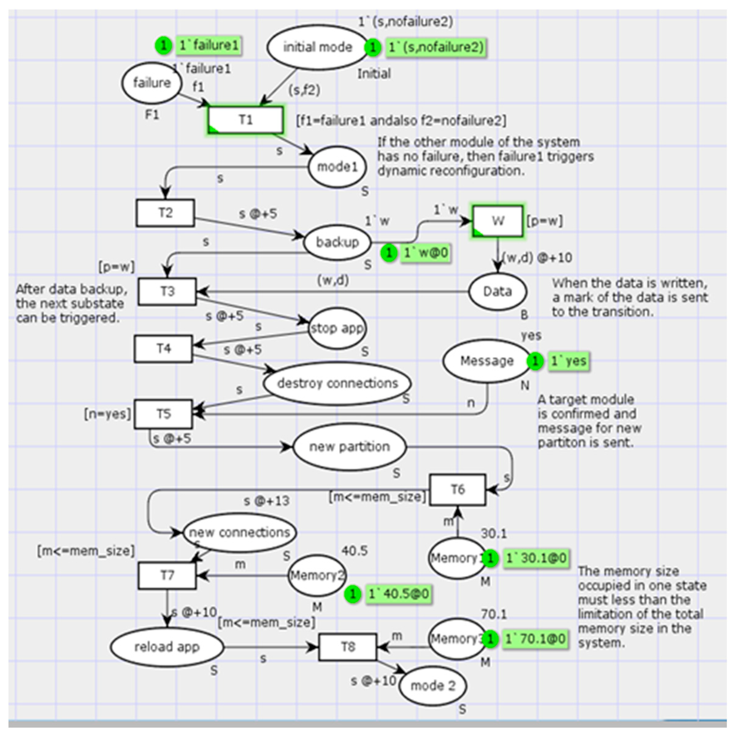
- After data backup for the process 1, process 1 is shut down and the connections of process 1 in the module N are destroyed.
- (2)
- The system selects a proper module to establish a new partition to run process 1. The strategy for selecting the target module is not introduced here. The target module is module D in this case.
- (3)
- A new partition is created in the target module D. Moreover, new channels and connections are set up. Process 1 is reloaded and restarted on the new partition in module D.
5.2. Simulation Results
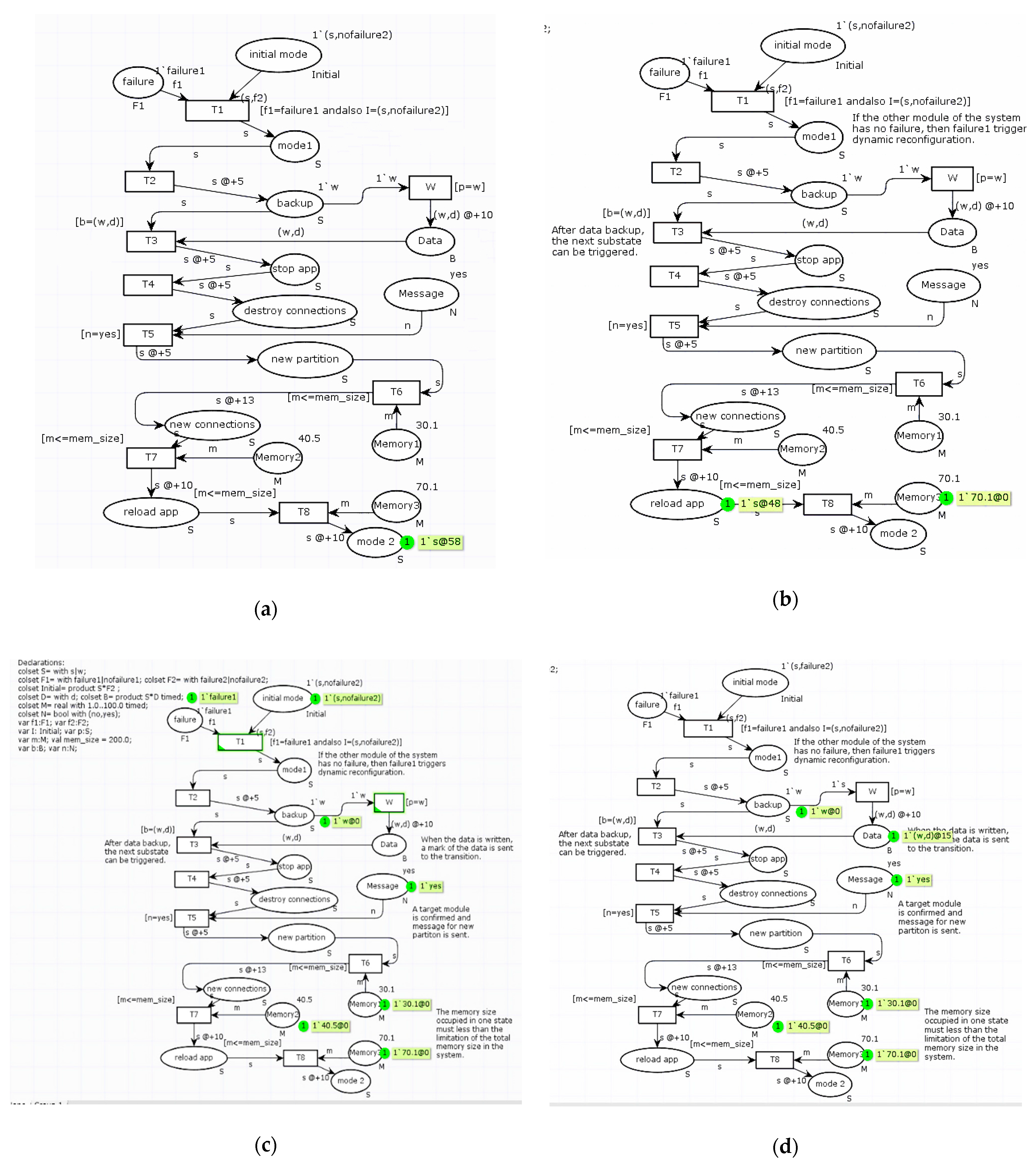
- Condition 2: Constraint of the memory size is not satisfied. The simulation will stop running when it runs for 48 ms, because the guard function [m ≤ mem_size] is not satisfied. The upper limit of the system memory size mem_size is only 70 M, but the state needs to occupy a memory size of 70.1 M, so the simulation ends. The result is shown in Figure 16b.
- Condition 3: Real-time constraint for the system state transition is not satisfied. By comparing the time consumed and real-time requirements, it can be shown whether the real-time constraint is satisfied.
- Condition 4: System state constraint for dynamic reconfiguration is not satisfied. When the system runs to transition T1, it can be judged by the guard function [f1 = failure1 and also I = (s, nofailure2)]. If fault propagation occurs before system reconfiguration and other modules are affected, the reconfiguration scheme cannot be adopted. The reconfiguration process stops and cannot be conducted, as shown in Figure 16c.
- Condition 5: Ability constraint for sharing data resources is not satisfied. When the system performs an operation of a shared data resource, if the forward state backup cannot write to the data component, then the checking of the data component and latter state are not triggered. Then, the process stops at a step of 15 ms, as shown in Figure 16d.
6. Conclusions
Author Contributions
Funding
Conflicts of Interest
References
- Airlines Electronic Engineering Committee. Avionics Application Software Standard Interface Part 1-Required Services; ARINC Document ARINC Specification 653 P1-3; Aeronautical Radio, Inc.: Annapolis, MD, USA, 2010. [Google Scholar]
- Standardization Agreement (STANAG), North Atlantic Treaty Organization (NATO). 4626-2005 Modular and Open Avionics Architecture (Part I: Architecture); North Atlantic Treaty Organization: Brussels, Belgium, 2005; pp. 24–34. [Google Scholar]
- Jolliffe, G. Producing a safety case for IMA blueprints. In Proceedings of the 24th Digital Avionics Systems Conference, Washington, DC, USA, 30 October–3 November 2005; IEEE: Piscataway, NJ, USA, 2005; Volume 2. [Google Scholar]
- López-Jaquero, V.; Montero, F.; Navarro, E.; Esparcia, A.; Catal’n, J.A. Supporting ARINC 653-based dynamic reconfiguration. In Proceedings of the 2012 Joint Working IEEE/IFIP Conference on Software Architecture and European Conference on Software Architecture, Helsinki, Finland, 20–24 August 2012; IEEE: Piscataway, NJ, USA, 2012. [Google Scholar]
- Bieber, P.; Noulard, E.; Pagetti, C.; Planche, T.; Vialard, F. Preliminary design of future reconfigurable IMA platforms. ACM Sigbed Rev. 2009, 6, 1–5. [Google Scholar] [CrossRef]
- Hilbrich, R.; van Kampenhout, R. Dynamic reconfiguration in NoC-based MPSoCs in the avionics domain. In Proceedings of the 3rd International Workshop on Multicore Software Engineering, ACM, New York, NY, USA, 1–8 May 2010. [Google Scholar]
- Ding, M. Research on Reconfiguration and Verification Methods for Integrated Modular Avionics. Ph.D. Thesis, Northwest University, Xi’an, China, 2019. [Google Scholar]
- Shukla, J.; Das, B.; Pant, V. Stability constrained optimal distribution system reconfiguration considering uncertainties in correlated loads and distributed generations. Int. J. Electr. Power 2018, 99, 121–133. [Google Scholar] [CrossRef]
- Ellis, S.M. Dynamic software reconfiguration for fault-tolerant real-time avionic systems. Microprocess. Microsyst. 1997, 21, 29–39. [Google Scholar] [CrossRef]
- van Vliet, J.C. Software Engineering-Principles and Practice, 3rd ed.; Wiley: Hoboken, NJ, USA, 2008. [Google Scholar]
- SAE. AS5506A: Architecture Analysis and Design Language (AADL) Version 2.0; SAE: Warrendale, PA, USA, 2009. [Google Scholar]
- SAE. AS5506 Annex: Behavior Specification V2.0; SAE: Warrendale, PA, USA, 2011. [Google Scholar]
- Yang, Z.; Hu, K.; Ma, D.; Bodeveix, J.; Pi, L.; Talpin, J. From AADL to timed abstract state machines: A verified model transformation. J. Syst. Softw. 2014, 93, 42–68. [Google Scholar] [CrossRef]
- Walker, M.; Reiser, M.O.; Tucci-Piergiovanni, S.; Papadopoulos, Y.; Lönn, H.; Mraidha, C.; Parker, D.; Chen, D.; Servat, D. Automatic optimisation of system architectures using EAST-ADL. Syst. Softw. 2013, 86, 2467–2487. [Google Scholar] [CrossRef]
- Feiler, P.H.; Gluch, D.P. Model-Based Engineering with AADL: An introduction to the SAE Architecture Analysis & Design Language; Addison-Wesley: Boston, MA, USA, 2012. [Google Scholar]
- Bozzano, M.; Cimatti, A.; Katoen, J.P.; Nguyen, V.Y.; Noll, T.; Roveri, M. Safety, dependability and performance analysis of extended AADL models. Comput. J. 2010, 54, 754–775. [Google Scholar] [CrossRef]
- Hugues, J.; Zalila, B.; Pautet, L.; Kordon, F. From the prototype to the final embedded system using the Ocarina AADL tool suite. ACM Trans. Embed. Comput. Syst. (TECS) 2008, 7, 42. [Google Scholar]
- Chkouri, M.Y.; Robert, A.; Bozga, M.; Sifakis, J. Translating AADL into BIP-application to the verification of real-time systems. In Proceedings of the International Conference on Model Driven Engineering Languages and Systems, Toulouse, France, 28 September–3 October 2008; Springer: Berlin/Heidelberg, Germany, 2008. [Google Scholar]
- Zhang, F.; Zhao, Y.; Ma, D.; Niu, W. Formal verification of behavioral AADL models by stateful timed CSP. IEEE Access 2017, 5, 27421–27438. [Google Scholar] [CrossRef]
- Zhao, Z.; Zhang, J.; Sun, Y.; Liu, Z. Modeling of Avionic Display System for Civil Aircraft Based on AADL, 2018; IEEE: Piscataway, NJ, USA, 2018; pp. 4121–4126. [Google Scholar]
- Liu, Z.; Zhao, Z. Modeling and Schedulability Verfication of IMA Partitioning Based on AADL, 2017; IEEE: Piscataway, NJ, USA, 2017; pp. 417–420. [Google Scholar]
- Liu, W. AADL Model Transformation and Verification. Master’s Thesis, Shaanxi Normal University, Xi’an, China, 2013. [Google Scholar]
- Wu, Y.; Li, S. AADL model based on TPN. Comput. Technol. Dev. 2014, 24, 88–91. [Google Scholar]
- Hadad, A.S.A.; Ma, C.; Ahmed, A.A.O. Formal Verification of AADL Models by Event-B. IEEE Access 2020, 8, 72814–72834. [Google Scholar] [CrossRef]
- Sendall, S.; Kozaczynski, W. Model transformation: The heart and soul of model-driven software development. IEEE Softw. 2003, 20, 42–45. [Google Scholar] [CrossRef]
- Cuadrado, J.S.; Guerra, E.; de Lara, J. Static analysis of model transformations. IEEE Trans. Softw. Eng. 2017, 43, 868–897. [Google Scholar] [CrossRef]
- Hu, K.; Zhang, T.; Yang, Z.; Tsai, W. Exploring AADL verification tool through model transformation. J. Syst. Architect. 2015, 61, 141–156. [Google Scholar] [CrossRef]
- Chkouri, M.Y.; Robert, A.; Bozga, M.; Sifakis, J. Translating AADL into BIPapplication to the Verification of Real-Time Systems, Models in Software Engineering; Springer: Berlin/Heidelberg, Germany, 2009; pp. 5–19. [Google Scholar]
- Berthomieu, B.; Bodeveix, J.P.; Chaudet, C.; Dal Zilio, S.; Filali, M.; Vernadat, F. Formal Verification of AADL Specifications in the Topcased Environment, Reliable Software Technologies–Ada-Europe 2009; Springer: Berlin/Heidelberg, Germany, 2009; pp. 207–221. [Google Scholar]
- Rugina, A.-E.; Kanoun, K.; Kaâniche, M. A System Dependability Modeling Framework Using AADL and GSPNs, Architecting Dependable Systems IV; Springer: Berlin/Heidelberg, Germany, 2007; pp. 14–38. [Google Scholar]
- Bozzano, M.; Cavada, R.; Cimatti, A.; Katoen, J.-P.; Nguyen, V.Y.; Noll, T.; Olive, X. Formal verification and validation of AADL models. In Proceedings of the Embedded Real-Time Software and Systems 2010 (ERTS 2010), Toulouse, France, 19–21 May 2010. [Google Scholar]
- Kabir, S.; Papadopoulos, Y. Applications of Bayesian networks and Petri nets in safety, reliability, and risk assessments: A review. Saf. Sci. 2019, 115, 154–175. [Google Scholar] [CrossRef]
- Luan, W.; Qi, L.; Zhao, Z.; Liu, J.; Du, Y. Logic Petri net synthesis for cooperative systems. IEEE Access 2019, 7, 161937–161948. [Google Scholar] [CrossRef]
- Jensen, K. Coloured Petri Nets. In Petri Nets: Central Models and Their Properties; Springer: Berlin/Heidelberg, Germany, 1987; pp. 248–299. [Google Scholar]
- Jensen, K. Coloured Petri Nets: Basic Concepts, Analysis Methods and Practical Use; Springer Science & Business Media: Berlin, Germany, 2013; Volume 1. [Google Scholar]
- Huber, P.; Jensen, K.; Shapiro, R.M. Hierarchies in coloured Petri nets. In Proceedings of the International Conference on Application and Theory of Petri Nets, Bratislava, Slovakia, 24–29 June 2018; Springer: Berlin/Heidelberg, Germany, 1989. [Google Scholar]
- Marsan, M.A.; Balbo, G.; Conte, G.; Donatelli, S.; Franceschinis, G. Modelling with Generalized Stochastic Petri Nets; John Wiley & Sons, Inc.: Hoboken, NJ, USA, 1994. [Google Scholar]
- Ajmone Marsan, M.; Conte, G.; Balbo, G. A class of generalized stochastic Petri nets for the performance evaluation of multiprocessor systems. ACM Trans. Comput. Syst. (TOCS) 1984, 2, 93–122. [Google Scholar] [CrossRef]
- Chiola, G.; Marsan, M.A.; Balbo, G.; Conte, G. Generalized stochastic Petri nets: A definition at the net level and its implications. IEEE Trans. Softw. Eng. 1993, 19, 89–107. [Google Scholar] [CrossRef]
- Bugarin, A.J.; Barro, S. Fuzzy reasoning supported by Petri nets. IEEE Trans. Fuzzy Syst. 1994, 2, 135–150. [Google Scholar] [CrossRef]
- Li, Y.; Chen, Y.; Tang, N.; Yang, L. Modeling and analysis of failure mechanism dependence based on petri net. In Proceedings of the Prognostics and System Health Management Conference, Chengdu, China, 19–21 October 2016; pp. 1–7. [Google Scholar]
- Wieland, C.; Schmid, O.; Meiler, M.; Wachtel, A.; Linsler, D. Reliability computing of polymer-electrolyte-membrane fuel cell stacks through petri nets. J. Power Sources 2009, 190, 34–39. [Google Scholar] [CrossRef]
- Sunanda, B.E.; Seetharamaiah, P. Modeling of safety-critical systems using petri nets. ACM SIGSOFT Softw. Eng. Notes 2015, 40, 1–7. [Google Scholar] [CrossRef]
- Li, W.; He, M.; Sun, Y.; Cao, Q. A novel layered fuzzy Petri nets modelling and reasoning method for process equipment failure risk assessment. J. Loss Prevent. Proc. 2019, 62, 103953. [Google Scholar] [CrossRef]
- Gonçalves, P.; Sobral, J.; Ferreira, L.A. Unmanned aerial vehicle safety assessment modelling through petri Nets. Reliab. Eng. Syst. Safe 2017, 167, 383–393. [Google Scholar] [CrossRef]
- Liu, R. Reliability Modeling of Integrated Modular Avionics System Platform Using AADL, and GSPN Analysis Method. Master’s Thesis, Civil Aviation University of China, Tianjin, China, 2016. [Google Scholar]
- Li, Z.; Wang, S.; Zhao, T.; Liu, B. A hazard analysis via an improved timed colored petri net with time–space coupling safety constraint. Chin. J. Aeronaut. 2016, 29, 1027–1041. [Google Scholar] [CrossRef]
- Arena, D.; Criscione, F.; Trapani, N. Risk assessment in a chemical plant with a CPN-HAZOP Tool. IFAC-PapersOnLine 2018, 51, 939–944. [Google Scholar] [CrossRef]
- Committee, A.E. ARINC 664 Aircraft Data Networks, Part7: Avionics Full Duplex Switched Ethernet (AFDX) Network; Aeronautical Radio, Inc.: Annapolis, MD, USA, 2005. [Google Scholar]
- Prisaznuk, P.J. ARINC 653 role in integrated modular avionics (IMA). In Proceedings of the 2008 IEEE/AIAA 27th Digital Avionics Systems Conference, St. Paul, MN, USA, 26–30 October 2008; IEEE: Piscataway, NJ, USA, 2008. [Google Scholar]
- Zhang, F.; Chu, W.; Fan, X.; Wan, M. Research on architecture of integrated modular avionics [J]. Electron. Opt. Control 2009, 9, 013. [Google Scholar]
- Reis, J.G.; Wanner, L.; Fröhlich, A.A. A framework for dynamic real-time reconfiguration. In Proceedings of the 2015 Euromicro Conference on Digital System Design (DSD), Funchal, Portugal, 26–28 August 2015; IEEE: Piscataway, NJ, USA, 2015. [Google Scholar]
- Aeronautical Radio. Avionics Application Software Standard Interface; ARINC653: Annapolis, MD, USA, 2010. [Google Scholar]
- Montano, G.; McDermid, J. Human Involvement in Dynamic Reconfiguration of Integrated Modular Avionics, Avionics. In Proceedings of the 27th Digital Avionics Systems Conference, St. Paul, MN, USA, 26–30 October 2008; IEEE: Piscataway, NJ, USA, 2008. [Google Scholar]
- Zhou, Q.; Gu, T.; Hong, R.; Wang, S. An AADL-based design for dynamic reconfiguration of DIMA. In Proceedings of the 2013 IEEE/AIAA 32nd Digital Avionics Systems Conference (DASC), East Syracuse, NY, USA, 5–10 October 2013; IEEE: Piscataway, NJ, USA, 2013. [Google Scholar]
- Montano, G.; Norridge, P.; Sullivan, W.; Topping, C.; Wishart, A.; Bubenhagen, F.; Fiethe, B.; Michalik, H.; Osterloh, B.; Ilstad, J. Dynamically Reconfigurable Processing Module for Future Space Applications. In Proceedings of the DASIA 2010 Data Systems In Aerospace, Budapest, Hungary, 1–4 June 2010; Volume 682. [Google Scholar]
- Suo, D.; An, J.; Zhu, J. A new approach to improve safety of reconfiguration in integrated modular avionics. In Proceedings of the 2011 IEEE/AIAA 30th Digital Avionics Systems Conference (DASC), Seattle, WA, USA, 16–20 October 2011; IEEE: Piscataway, NJ, USA, 2011. [Google Scholar]
- Arshad, N. Dynamic Reconfiguration of Software Systems Using Temporal Planning. Ph.D. Thesis, University of Colourado, Boulder, CO, USA, 2003. [Google Scholar]
- Montano, G. Dynamic Reconfiguration of Safety-Critical Systems: Automation and Human Involvement. Ph.D. Thesis, University of York, York, UK, 2011. [Google Scholar]
- Quan, Z.; Wang, S. IMA reconfiguration modelling and reliability analysis based on AADL. In Proceedings of the 4th Annual IEEE International Conference on Cyber Technology in Automation, Control and Intelligent, Hong Kong, China, 4–7 June 2014; IEEE: Piscataway, NJ, USA, 2014. [Google Scholar]
- Suo, D.; An, J.; Zhu, J. AADL-based modelling and TPN-based verification of reconfiguration in integrated modular avionics. In Proceedings of the 2011 18th Asia Pacific Software Engineering Conference (APSEC), Ho Chi Minh, Vietnam, 5–8 December 2011; IEEE: Piscataway, NJ, USA, 2011. [Google Scholar]
- Aerospace, S.A.E. SAE Architecture Analysis and Design Language (AADL); Society of Automotive Engineers (SAE) International: Houston, TX, USA, 2009. [Google Scholar]
- Feiler, P.H.; Gluch, D.P.; Hudak, J.J. The Architecture Analysis & Design Language (AADL): An Introduction; No. CMU/SEI-2006-TN-011; Carnegie-Mellon Univ Pittsburgh PA Software Engineering Inst: Pittsburgh, PA, USA, 2006. [Google Scholar]
- Murata, T. Petri nets: Properties, analysis and applications. Proc. IEEE 1989, 77, 541–580. [Google Scholar] [CrossRef]
- Petri, C.A. Kommunikation mit Automaten. Bonn: Institute fur Instrumentelle Mathematik, Schriften des IIM Nr.3, 1962. Also, English Translation: Communication with Automata. Tech. Rep. RADC-TR-65–377 1966, 1, 253–279. [Google Scholar]
- Jensen, K. Coloured Petri nets: A high level language for system design and analysis. In Proceedings of the International Conference on Application and Theory of Petri Nets, Bonn, Germany, 1–5 June 1989; Springer: Berlin/Heidelberg, Germany, 1989. [Google Scholar]
- Kristensen, L.M.; Christensen, S.; Jensen, K. The practitioner’s guide to coloured Petri nets. Int. J. Softw. Tools Technol. Transf. (STTT) 1998, 2, 98–132. [Google Scholar] [CrossRef]
- Jensen, K.; Munkegade, N. An introduction to the theoretical aspects of coloured Petri nets. In Lecture Notes in Computer Science; Springer: Berlin/Heidelberg, Germany, 1994; Volume 803. [Google Scholar]
- Jensen, K.; Kristensen, L.M.; Wells, L. Coloured Petri Nets and CPN Tools for modelling and validation of concurrent systems. Int. J. Softw. Tools Technol. Transf. 2007, 9, 213–254. [Google Scholar] [CrossRef]
- Van der Aalst, W.M. The application of Petri nets to workflow management. J. Circuits Syst. Comput. 1998, 8, 21–66. [Google Scholar] [CrossRef]
- STANAG, NATO. 4626-2005 Modular and Open Avionics Architecture (Part VI: Guidelines for System Issues); Volume 4: System Configuration/Reconfiguration page: 7–20; North Atlantic Organization: Brussels, Belgium, 2005. [Google Scholar]
- Feiler, P.H.; Lewis, B.A.; Vestal, S. The SAE Architecture Analysis & Design Language (AADL) a standard for engineering performance critical systems. In Proceedings of the 2006 IEEE Conference on Computer Aided Control System Design, 2006 IEEE International Conference on Control Applications, 2006 IEEE International Symposium on Intelligent Control, Munich, Germany, 4–6 October 2006; IEEE: Piscataway, NJ, USA, 2006. [Google Scholar]
- SEI AADL Team. An Extensible Open Source AADL Tool Environment (OSATE); Software Engineering Institute: Pittsburgh, PA, USA, 2006. [Google Scholar]
- Beaudouin-Lafon, M.; Mackay, W.E.; Jensen, M.; Andersen, P.; Janecek, P.; Lassen, M.; Lund, K.; Mortensen, K.; Munck, S.; Ratzer, A.; et al. CPN/Tools: A tool for editing and simulating coloured petri nets ETAPS tool demonstration related to TACAS. In Proceedings of the International Conference on Tools and Algorithms for the Construction and Analysis of Systems, Genova, Italy, 2–6 April 2001; Springer: Berlin/Heidelberg, Germany, 2001. [Google Scholar]


| Error Level | Examples of Errors | Response Mechanism |
|---|---|---|
| Module Level |
|
|
| Partition Level |
|
|
| Process Level |
|
|
| No | Original Conditions | Simulation Results | Analyzing |
|---|---|---|---|
| 1 | Val mem_size = 200.0 (Figure 16a) | Simulation finish well | Memory constraints for system state is fulfilled. |
| 2 | Val mem_size = 70.0 (Figure 16b) | T8 can’t be fired, simulation stop | Memory constraints for system state don’t meet the requirements. |
| 3 | Time cost during the simulation beyond the real-time constraint | The time stamp ‘@ + 48′ reveals the running time 48 beyond the limitation 30. | Real-time constraints for system state transition is not satisfied. |
| 4 | 1‘(s, failure2) - > initial mode and 1‘failure1 - > failure (Figure 16c) | The simulation not running, T1 is not fired | The system is in a fault propagation state and not fit for reconfiguration. |
| 5 | There is no ‘w’ sending to the place named Data (Figure 16d) | Value of guard function [p = w] is false. W is not fired. Simulation stop | A demanding mark is not written to data. components, so the next state failed to share the data. |
© 2020 by the authors. Licensee MDPI, Basel, Switzerland. This article is an open access article distributed under the terms and conditions of the Creative Commons Attribution (CC BY) license (http://creativecommons.org/licenses/by/4.0/).
Share and Cite
Jiang, Z.; Zhao, T.; Wang, S.; Ju, H. New Model-Based Analysis Method with Multiple Constraints for Integrated Modular Avionics Dynamic Reconfiguration Process. Processes 2020, 8, 574. https://doi.org/10.3390/pr8050574
Jiang Z, Zhao T, Wang S, Ju H. New Model-Based Analysis Method with Multiple Constraints for Integrated Modular Avionics Dynamic Reconfiguration Process. Processes. 2020; 8(5):574. https://doi.org/10.3390/pr8050574
Chicago/Turabian StyleJiang, Zeyong, Tingdi Zhao, Shihai Wang, and Hongyan Ju. 2020. "New Model-Based Analysis Method with Multiple Constraints for Integrated Modular Avionics Dynamic Reconfiguration Process" Processes 8, no. 5: 574. https://doi.org/10.3390/pr8050574
APA StyleJiang, Z., Zhao, T., Wang, S., & Ju, H. (2020). New Model-Based Analysis Method with Multiple Constraints for Integrated Modular Avionics Dynamic Reconfiguration Process. Processes, 8(5), 574. https://doi.org/10.3390/pr8050574