Synthesis of Large-Scale Bio-Hydrogen Network Using Waste Gas from Landfill and Anaerobic Digestion: A P-Graph Approach

Abstract

Due to the expanding concern on cleaner production and sustainable development aspects, a technology shift is needed for the hydrogen production, which is commonly derived from natural gas. This work aims to synthesise a large-scale bio-hydrogen network in which its feedstock, i.e., bio-methane, is originated from landfill gas and palm oil mill effluent (POME). Landfill gas goes through a biogas upgrader where high-purity bio-methane is produced, while POME is converted to bio-methane using anaerobic digestor (AD). The generated bio-methane is then distributed to the corresponding hydrogen sink (e.g., oil refinery) through pipelines, and subsequently converted into hydrogen via steam methane reforming (SMR) process. In this work, P-graph framework is used to determine a supply network with minimum cost, while ensuring the hydrogen demands are satisfied. Two case studies in the West and East Coasts of Peninsular Malaysia are used to illustrate the feasibility of the proposed model. In Case Study 1, four scenarios on the West Coast have been considered, showing total cost saving ranging between 25.9% and 49.5%. This showed that aside from the positive environmental impact, the incorporation of bio-hydrogen supply can also be economically feasible. Such benefits can also be seen in Case Study 2, where the uptake of biogas from landfill and POME sources on the East Coast can lead to a 31% reduction on total network cost. In addition, the effect of bio-hydrogen supply network on carbon footprint reduction was analysed in this work.

1. Introduction

Global warming is the main driving force for researchers in finding ways to curb greenhouse gas (GHGs) emissions. A growing number of countries are paving ways for sustainable future by turning to renewable energy [1]. Another source of energy that has been gaining interest globally is hydrogen. The latter has been widely recognised as a future energy carrier due to factors such as being environmental-friendly and consisting of high-energy capacity; it can be synthesised using diverse resources (including renewable energy sources). In the chemical process industries, hydrogen is a common feedstock for ammonia and methanol, as well as for oil refineries [2]. In addition, hydrogen is a promising fuel source for transportation. Among the various hydrogen production technologies, steam methane reforming (SMR) remains the most well established process for hydrogen production [3]. It is anticipated that by the year 2030, 40% of the global hydrogen production will be generated via SMR process, dominating other routes such as electrolysis, gasification, and partial oxidation process [4]. The conventional SMR process utilises natural gas as feedstock and often leads to gigantic GHG emissions, leading to low sustainability [5]. This drives the research to seek for a more sustainable hydrogen production process, which considers both the environmental aspect as well as the scalability of the process. Hydrogen productions from biological sources, such as biomass or biogas, has received good attention since it is eco-friendly, as compared to the conventional SMR process [6].

Biogas consists of a large portion of methane, which acts as a good replacement for natural gas. In the seminal work, Hwangbo et al. [7] proposed a hydrogen production network for South Korea using mathematical programming (MP) approach, in which biogas from wastewater treatment plant is used as the main resource. Alternatively, landfill gas is another potential source for biogas production. In the compacted and covered environment of landfills, anaerobic bacteria decompose the municipal solid waste (MSW), which results in the generation of methane and carbon dioxide [8]. In the Malaysian context, daily waste generation has been estimated as 0.5–0.8 kg per capita in the rural area, while the amount is double in the urban areas [9]. Besides, it is predicted that MSW in Malaysia will achieve 31,000 t/d in year 2020, and further increase to 51,700 t/d by year 2025 [9]. Therefore, there is a need to treat or valorise the landfill gas in order to prevent it from emitting into the atmosphere. It is possible to harness heat and electricity from the produced landfill gas by channelling it to combustion engines or alternator [10,11]. In a recent work, Hoo et al. [12] explored the potential of the integration of bio-methane into existing natural gas grid in Malaysia for power generation. However, due to limitations of the local electricity load demand, the captured landfill gas is under-utilised. Thus, the use of landfill gas for hydrogen generation becomes an attractive option for bio-methane utilisation in Malaysia.

Malaysia is the second largest producer of palm oil in the world, accounting for 39% of world palm oil production and 44% of world exports [13]. However, the mass production of palm oil further leads to a gigantic generation of oil palm waste, which accounted for about 86% of the total biomass available in the country [14]. Among the palm oil wastes, palm oil mill effluent (POME) is the largest contributor. Although it is non-toxic, it still poses a severe environmental issue due to its large oxygen depleting capabilities [15]. Fortunately, due to its high organic content, POME can serve as a prominent source for methane generation via anaerobic digestion (AD). Similar to landfill gas, the generated bio-methane can then be converted into hydrogen through SMR process. Therefore, a bio-hydrogen supply network that incorporates the use of biogas (from landfill and AD process) should be considered to improve the sustainability of the existing network.

Several models have been reported on hydrogen production from biogas sources. Borisov et al. [16] developed a model that describes the simultaneous production of methane and hydrogen from AD of organic waste. A study by Woo et al. [17] demonstrated optimal design and operation of four types of biomass in a hydrogen supply chain. In addition, Hwangbo et al. [6] utilized MP for hydrogen production from biogas under demand uncertainty. On the other hand, Robles et al. [18] modelled the demand uncertainty in a hydrogen supply network with fuzzy MP. More recently, MP was used to determine a sustainable hydrogen supply network with the consideration of fuelling station planning [19]. Most of these models are developed using MP, where only a single solution is produced unless further constraints are added to the model [20]. Besides, model solving with the conventional method becomes progressively difficult as the problem size increases [21].

A bio-hydrogen network is considerably a large network, as it includes (i) the decision of selecting the feedstock for hydrogen production—either natural gas or biogas obtained through landfill/AD process; and (ii) the decision of locating the compressor sub-stations between the sources and sinks. Therefore, to solve this network problem across a country, a rigorous combinatorial tool called P-graph [22] is used. P-graph determines and showcases the maximal structure of a given network, and aids in visualising the full network model. It was developed by Friedler et al. [23] to solve the process network synthesis problem. In general, its feature, which exploits the combinatorial nature of the problem instead of transforming it into a set of equations, is the key advantage of P-graph over other conventional MP approaches [24]. Coupled with three algorithms [25] and five axioms [23] embedded in the P-graph framework, it is capable to perform rigorous combinatorial computation tasks efficiently [26]. It is capable to provide multiple feasible network structures simultaneously, which had proved invaluable in various works. For instance, Voll et al. [27] utilised this additional information to yield rational decisions for a given network. Lam et al. [28], on the other hand, identified the bottleneck of a given technology, while near-optimal criteria weights were considered by Low et al. [29] during the evaluation of various negative emission technologies. The P-graph framework is explained in depth in Section 3.

In this works, P-graph approach is utilised to synthesise an optimal bio-hydrogen network, which integrate the use of landfill gas and POME into the conventional hydrogen supply network. This work contributes in: (i) extending the P-graph methodology to solve hybrid bio-hydrogen network that incorporates the use of two biogas sources (landfill gas and POME) in Malaysia; and (ii) evaluating the feasibility of such hybrid hydrogen production network.

The paper is structured as follows. In the following section, a clear problem statement is defined. The research methodology is presented in Section 3, while the descriptions of the two case studies are presented in Section 4. The obtained results are then shown and analysed in Section 5, before the work is finally concluded.

2. Problem Statement

Given the biogas capacities of landfill sites and POME sources, a bio-hydrogen supply network is to be synthesised. This alternative method reduces the dependency of hydrogen production on non-renewable fossil fuels. In addition, it prevents the emissions of methane from landfill gas and biogas (obtained from the AD treatment of POME) to the atmosphere. Each landfill gas source i (i = 1, 2, …, n) is equipped with a biogas upgrader to produce clean bio-methane. Whereas, POME sources k (k = 1,2, …, n) goes through anaerobic digestion (AD) process and is converted to bio-methane. Each hydrogen sink j (j = 1, 2, …, n) is connected to bio-methane supply through pipelines. Compressor substations, l (l = 1, 2, …, n) are located in between the sources and the sinks for the re-compression of gas. Using the SMR process on-site, the bio-methane is converted to hydrogen. The main objective of the model is to determine an optimal bio-hydrogen supply network with minimum cost, while ensuring all hydrogen demand targets of the sinks are met. Figure 1 shows an overview of the proposed model.

3. Methodology

P-graph is a directed bipartite (multicomponent) graph that represents the structure of a process system [30]. The direction of the arcs represents the direction of the materials flow in the network of the process system. The method for optimising a complex network has traditionally relied on MP. However, as aforementioned, applying MP for large problems becomes progressively difficult [31]. Moreover, in some complex cases, MP is time consuming, error-prone and may miss advantageous options. The structural infeasibilities in the evaluated combinations are discovered by the solvers only after evaluating the constraints. Therefore, practical problems often become too complex to solve. In the case where the problem is simplified to be solvable, the resulting formulation is usually no longer representative of the original task [31]. The P-graph framework [23] was then been developed to address these combinatorial challenges for optimising process networks. The recent works done by Cabezas et al. [32] on design and engineering of sustainable process system, Lam et al. [33] on creating biomass network, and Vance et al. [34] on designing sustainable energy supply chains are some of the examples that attempted to address supply chain issues using P-graph methodology. P-graph is capable of unambiguously representing process structures for sequential, parallel, and alternative activities. In addition to graphical representation, the P-graph framework provides a set of rigorous and effective algorithms for supply chain network synthesis [22]. A considerable advantage of the P-graph model is its potential in solving real life industrial problems related to the design of supply chain, while incorporating various process-engineering problems, such as reaction and separation engineering and transportation operations. The P-graph model evaluates the maximal structure and generates feasible optimised results, which can be ranked based on certain parameters, such as cost and energy potential. A general direction of the P-graph is from input materials to operating units and from operating units to its output materials. The vertices used in the P-graph are denoted as operating units and materials. The vertices used for materials have several different types or subsets such as raw materials, which is the input elements of the entire process, product materials, which gather the required input and represents the results of the process, and lastly, the intermediate materials, which are the elements generated or used in between processing phases. Meanwhile, operating units are required to carry out certain tasks in between processing phases [22]. The applied operating unit and materials element notations in P-graph are represented in

Table 1. Representation of Symbols used in P-graph Studio.

	Raw Material/Supply/Source		Final Product/Demand
	Intermediate Material		Operating Unit

. The P-graph framework is based on the five axioms below [23]:

• Every final product is represented in the graph.
• A vertex of the M-type has no input if and only if it represents a raw material.
• Every vertex of the O-type represents an operating unit defined in the synthesis problem.
• Every vertex of the O-type has at least one path leading to a vertex of the M-type representing a final product
• If a vertex of the M-type belongs to the graph, it must be an input to or output from at least one vertex of the O-type in the graph.

P-graph uses three main algorithms, which are explained below:

• Maximal Structure Generation (MSG): This algorithm identifies the maximal structure of the network, which is based on five axioms and represents the union of all possible networks [26].
• Solution Structure Generation (SSG): This algorithm determines all combinatorial feasible networks, which are the subsets of maximal structure [25].
• Accelerated Brand and Bound (ABB): This algorithm optimises the network efficiently, which excludes search of infeasible and redundant network structures. As a result, both the search space and computational effort are typically reduced, significantly, compared to the conventional branch-and-bound algorithm [35].

The detailed explanation and demonstration of the P-graph framework is given in the following subsections.

3.1. Development of P-Graph Model for Large-Scale Bio-Hydrogen Network

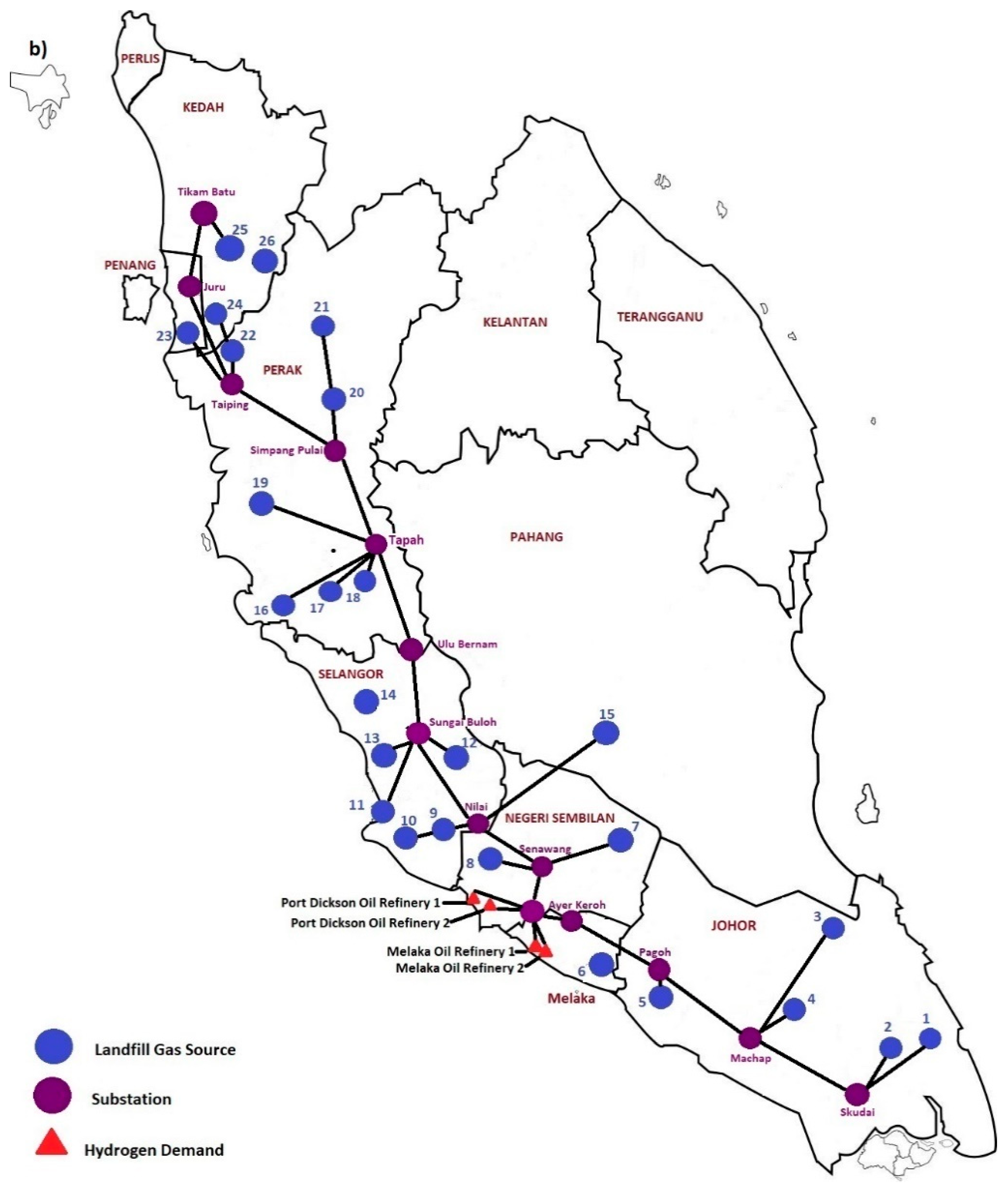
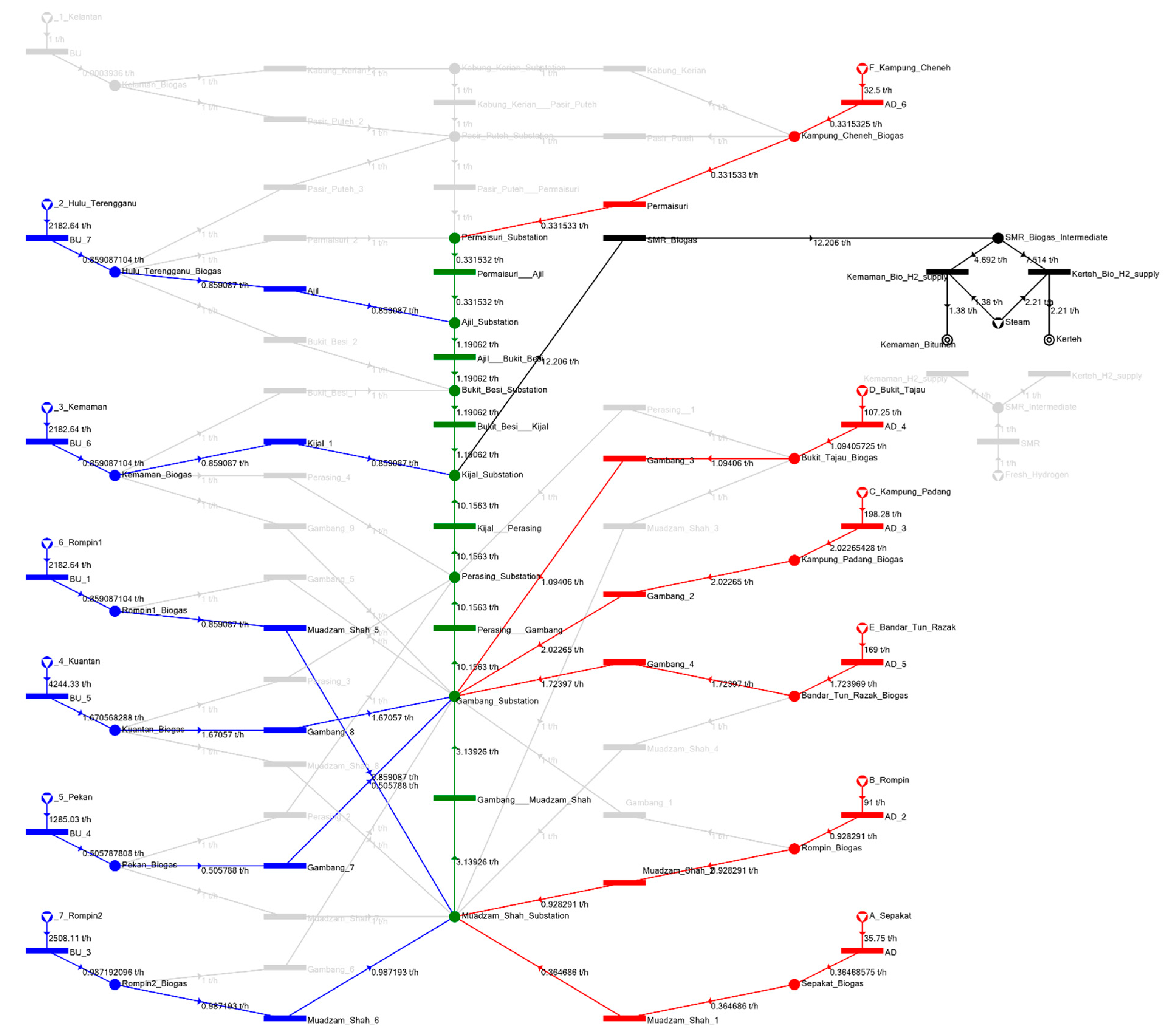
In the process to produce bio-methane, the captured landfill gas goes through biogas upgrader to increase its purity. The clean bio-methane is then compressed and transported through pipelines to the suitable substation for further recompression. The bio-methane flows through the pipelines and is delivered to hydrogen sinks. Finally, the collected gas will be fed into SMR to produce hydrogen. On the other hand, POME sources also follow the similar path as landfill gas with a small difference that POME source will be converted into bio-methane via AD instead of being fed to biogas upgrader. P-graph framework is utilised to obtain the most economically feasible route that can fulfil the demand of the hydrogen sinks. The procedure for the bio-hydrogen network synthesis follows the flowchart illustrated in Figure 2. To apply the P-graph approach, various information has to be pre-determined and specified (see detailed information in case study section).

As the initial step, the available landfill and POME sites are identified (Layer 1). As shown in Figure 3, the sources (in green) are connected to biogas upgraders (BGUG) or AD in order to produce bio-methane (Layer 2, in orange). The investment and operating costs of BGUG and AD are the input of its operating unit. The generated bio-methane is represented as the M-vertex (in blue), while the conversion ratio of landfill gas to bio-methane and POME to bio-methane are defined along the corresponding arcs. The second operating unit (in purple), accounts for the compressor and pipeline costs for sending bio-methane to the substations (Layer 3).

To ensure that bio-methane flows through the pipelines optimally, it must be periodically compressed and pushed through the pipeline (see Figure 4). Thus, each bio-methane source is connected to several substations located within an 80 km radius distance from the source [36]. P-graph will then decide what substation the bio-methane should be delivered to, based on the overall operating and capital costs. Note that the compressor and pipeline costs are input to the O-vertex (in maroon; Layer 4). From Figure 4, “Substation 6” is served as the last substation that is located near to the hydrogen sink. In other words, bio-methane collected from the South region will be transferred upwards, while the bio-methane collected from the North region will be delivered downward, in order to approach this “final station”. Note that the substation arrangement shown in Figure 4 is merely an illustrative example. It can be changed according to the specific case study.

Finally, the collected bio-methane will be distributed to the hydrogen sinks. For illustration purposes, four hydrogen demand sites are shown in Figure 5. The distribution of bio-methane to each demand site is determined by P-graph. Note that the grey O-vertex represents the SMR processes, which convert the bio-methane into bio-hydrogen (Layer 5). In the case where the produced bio-hydrogen is insufficient to cover the hydrogen demand, fresh hydrogen from conventional fossil fuel (i.e., brown M-vertex) can be purchased from third parties. Note that the model might decide not to produce bio-hydrogen if the fresh hydrogen from conventional fossil fuel is much cheaper (Layer 6).

3.2. Model Formulation

This section summarises the mathematical formulations that are embedded in the constructed P-graph model.

3.2.1. Network Design

Equation (1) describes the demand of hydrogen ($F_j^{H2}$, t/h) in each sink $j$. The hydrogen demand of the latter can be fulfilled by fresh hydrogen ($F_j^{FH2}$, t/h) and/or produced bio-hydrogen ($F_j^{BH2}$, t/h). The latter can be mathematically expressed as Equation (2):

$$F_j^{H2}=F_j^{BH2}+F_j^{FH2} \forall j$$

(1)

$$F_j^{BH2}=\frac{{\sum }_l{F}_{l,j}^{CH4}}{X^{SMR}} \forall j$$

(2)

where $F_{l,j}^{BH2}$ refers to the flowrate of bio-methane sent to hydrogen sink j from substation l (t/h); while $X^{SMR}$ represents the methane-to-hydrogen conversion ratio (kg CH₄/kg H₂).

Equations (3) and (4) express the mass balance constraint across the sources, where $F_i^{CH4}$ (t/h) and $F_k^{CH4}$ (t/h) denote the bio-methane generated from landfill source i and POME source k respectively; while $F_{i,l}^{CH4}$ (t/h) and $F_{k,l}^{CH4}$ (t/h) refer to the methane flowrate sent from each source to substation l.

$$F_i^{CH4}={{\displaystyle \sum }}_l{F}_{i,l}^{CH4} \forall l$$

(3)

$$F_k^{CH4}={{\displaystyle \sum }}_l{F}_{k,l}^{CH4} \forall l$$

(4)

On the other hand, the mass balance across the substations is presented in Equation (5), where $F_{l,l\prime }^{CH4}$ refers to the methane flowrate transported from substation l to another substation l’ (t/h).

$${{\displaystyle \sum }}_i{F}_{i,l}^{CH4}+{{\displaystyle \sum }}_k{F}_{k,l}^{CH4}={{\displaystyle \sum }}_{l\prime }{F}_{l,l\prime }^{CH4}+{{\displaystyle \sum }}_j{F}_{l,j}^{CH4} \forall l$$

(5)

Next, the conversion of landfill gas and POME to bio-methane modelled in P-graph can also be expressed mathematically. Due to the corrosive nature of landfill gas impurities, it is essential to improve methane purity via the biogas-upgrading unit prior to its delivery to the compressor substation. In this work, a high-pressure water scrubber is used as the biogas-upgrading unit. Water scrubbing can remove carbon dioxide and hydrogen sulphide since these components are more soluble in water than methane [37]. Depending on the type of waste available in the landfill site, landfill gas ($F_i^{LF}$, in t/h) generally contains 50–60 volume% methane [12]. Therefore, the methane capacity in each source i can be assumed as follows:

$$F_i^{CH4}\le F_i^{LF}\times X_i^{LF} \forall i$$

(6)

where $X_i^{LF}$ refers to the landfill gas-to-bio-methane conversion in terms of mass flowrate (wt.%). On the other hand, POME can be converted into bio-methane via AD process. Its conversion can be formulated as Equation (7):

$$F_k^{CH4}\le F_k^{POME}\times X_i^{POME} \forall k$$

(7)

where $F_k^{POME}$ refers to the available POME capacity in source k (m³/h); while $X_k^{POME}$ refers to the conversion ratio of AD process (t CH₄/m³ POME).

3.2.2. Objective Function

The main objective of the model is to determine a bio-hydrogen network with minimum total annualised cost ($TAC$, $/y). It is generally the sum of annual operating cost ($AOC$, $/y), annualised investment cost ($AIC$, $/y) and annual raw material cost ($AMC$, $/y), given as in Equation (8).

$$TAC=AOC+AIC+AMC$$

(8)

where $AOC$ is the product of the operating cost ($OC$, $/y) and annual operating hours ($AOH$), given as in Equation (9). Note that $OC$ encompasses of the operating cost of the involved operating units (Equation (10)):

$$AOC=OC\times AOH$$

(9)

$$\begin{array}{c}OC={{\displaystyle \sum }}_i\frac{F_i^{CH4}}{X_i^{LF}}\times {\mathrm{UOC}}^{BGU}+{{\displaystyle \sum }}_k\frac{F_k^{CH4}}{X_k^{POME}}\times {\mathrm{UOC}}^{AD}+({{\displaystyle \sum }}_i{{\displaystyle \sum }}_l{F}_{i,l}^{CH4}+{{\displaystyle \sum }}_k{{\displaystyle \sum }}_l{F}_{k,l}^{CH4}\\ +{{\displaystyle \sum }}_{l^{\prime }}{{\displaystyle \sum }}_l{F}_{l^{\prime },l}^{CH4})\times {\mathrm{UOC}}^{Comp}+{{\displaystyle \sum }}_l{{\displaystyle \sum }}_j{F}_{l,j}^{CH4}\times {\mathrm{UOC}}^{SMR}\end{array}$$

(10)

where ${\mathrm{UOC}}^{BGU}$, ${\mathrm{UOC}}^{AD}$, ${\mathrm{UOC}}^{Comp}$ and ${\mathrm{UOC}}^{SMR}$ refer to the unit operating costs for biogas upgrader ($.h/t), AD ($.h/m³), compressor($.h/t), and SMR ($.h/t)units respectively.

The $AIC$($/y), on the other hand, is a ratio of total investment cost ($TIC$, $) over the life span of the plant ($LS$).

$$AIC=\frac{TIC}{LS}$$

(11)

The $TIC$ ($/h) considers the investment costs of biogas upgrader (${\mathrm{IC}}^{BGU}$, $/h), AD (${\mathrm{IC}}^{AD}$, $/h), compressor (${\mathrm{IC}}^{Comp}$, $/h), pipeline (${\mathrm{IC}}^{Pipe}$, $/h), and the SMR process (${\mathrm{IC}}^{SMR}$, $/h). These parameters can be computed using Equations (12)–(17):

$$TIC={\mathrm{IC}}^{BGU}+{\mathrm{IC}}^{AD}+{\mathrm{IC}}^{Comp}+{\mathrm{IC}}^{SMR}+{\mathrm{IC}}^{Pipe}$$

(12)

$${\mathrm{IC}}^{BGU}={{\displaystyle \sum }}_i\frac{F_i^{CH4}}{X_i^{LF}}\times {\mathrm{UIC}}^{BGU}$$

(13)

$${\mathrm{IC}}^{AD}={{\displaystyle \sum }}_k\frac{F_k^{CH4}}{X_k^{POME}}\times {\mathrm{UIC}}^{AD}$$

(14)

$${\mathrm{IC}}^{Comp}=\left({{\displaystyle \sum }}_i{{\displaystyle \sum }}_l{F}_{i,l}^{CH4}+{{\displaystyle \sum }}_k{{\displaystyle \sum }}_l{F}_{k,l}^{CH4}+{{\displaystyle \sum }}_{l^{\prime }}{{\displaystyle \sum }}_l{F}_{l^{\prime },l}^{CH4}\right)\times {\mathrm{UIC}}^{Comp}$$

(15)

$${\mathrm{IC}}^{SMR}={{\displaystyle \sum }}_l{{\displaystyle \sum }}_j{F}_{l,j}^{CH4}\times {\mathrm{UIC}}^{SMR}$$

(16)

$${\mathrm{IC}}^{Pipe}=\left({{\displaystyle \sum }}_i{{\displaystyle \sum }}_l{d}_{i,l}+{{\displaystyle \sum }}_k{{\displaystyle \sum }}_l{d}_{k,l}+{{\displaystyle \sum }}_l{{\displaystyle \sum }}_{l^{\prime }}{d}_{l,l^{\prime }}+{{\displaystyle \sum }}_l{{\displaystyle \sum }}_j{d}_{l,j}\right)\times {\mathrm{UIC}}^{Pipe}$$

(17)

where ${\mathrm{UIC}}^{BGU}$, ${\mathrm{UIC}}^{AD}$, ${\mathrm{UIC}}^{Comp}$, ${\mathrm{UIC}}^{SMR}$, and ${\mathrm{UIC}}^{Pipe}$ refer to the unit operating costs for biogas upgrader ($/t), AD ($/m³), compressor ($/t), SMR ($/t), and pipeline (t/km), respectively.

The $AMC$ ($/y) in Equation (8) is a product of total flow rate of external hydrogen supply ($F_j^{FH2}$, t/h), its unit cost (${\mathrm{C}}^{H2}$, $/t H₂), and $AOH$.

$$AMC={{\displaystyle \sum }}_j{F}_j^{FH2}\times {\mathrm{C}}^{H2}\times AOH$$

(18)

The above is an LP model, which may be solved to achieve global solution, if the solution exists.

4. Case Studies

Two case studies based at Malaysia scenarios will be used to demonstrate the proposed P-graph framework. Case Study 1 focused on the West Coast of Peninsular Malaysia, which only considers landfill gas as the bio-methane source. On the other hand, Case Study 2 is based on the East Coast of Peninsular Malaysia, where both landfill gas and POME are utilised as the bio-methane feedstock. The economic parameters used in these case studies are the same, and are summarised in

Table 2. Economic parameters for case studies.

Parameters	Price	Unit	Reference
${\mathrm{UIC}}^{BGU}$	7,459,658	$/t landfill gas/h	[38]
${\mathrm{UOC}}^{BGU}$	83	$/t landfill gas/h
${\mathrm{UIC}}^{AD}$	6540	$/m3	[39]
${\mathrm{UOC}}^{AD}$	0.0872	$/m3/CH4/h	[40]
${\mathrm{UIC}}^{Comp}$	827,613	$/t CH4
${\mathrm{UOC}}^{Comp}$	2.78	$/t CH4/h	[41]
${\mathrm{UIC}}^{Pipe}$	65,940	$/km	[42]
${\mathrm{C}}^{H2}$	4880	$/t H2	[43]
${\mathrm{UIC}}^{SMR}$	42,104	$/t CH4
${\mathrm{UOC}}^{SMR}$	0.4	$/t CH4/h
$X_i^{LF}$	25–30	weight%	[12]
$X_k^{POME}$	0.01	t CH4/m3 POME	[44]
$X^{SMR}$	3.4	kg CH4/kg H2	[7]
$AOH$	7200	h/y	-
$OY$	10	y	-

${\mathrm{UOC}}^{BGU}$, ${\mathrm{UOC}}^{AD}$, ${\mathrm{UOC}}^{Comp}$ and ${\mathrm{UOC}}^{SMR}$ refer to the unit operating costs for biogas upgrader, AD, compressor, and SMR units respectively; ${\mathrm{UIC}}^{BGU}$, ${\mathrm{UIC}}^{AD}$, ${\mathrm{UIC}}^{Comp}$, ${\mathrm{UIC}}^{SMR}$, and ${\mathrm{UIC}}^{Pipe}$ refer to unit operating costs for biogas upgrader, AD, compressor, SMR, and pipeline, respectively; $X_k^{POME}$ refers to the conversion ratio of AD process, $X_i^{LF}$ refers to the landfill gas-to-bio-methane conversion.

. This LP model for both case studies were solved using the ABB algorithm in P-graph solver.

4.1. Case Study 1

In this case study, landfill gas is used as bio-methane source for four main oil refineries on the West Coast of Peninsular Malaysia (see Figure 6), with their capacities and hydrogen demand tabulated in

Table 3. Landfill gas capacity and hydrogen demand of each region (Case Study 1).

States	Label	Regions	Landfill Gas Capacity (t/h) a	Hydrogen Demand (t/h) b
Johor	1	Kota Tinggi	8.77	-
	2	Kulai	2.36	-
	3	Kluang 1	1.90	-
	4	Kluang 2	6.31	-
	5	Batu Pahat	7.10	-
Melaka	6	Jasin	2.36	-
	S1	Melaka Oil Refinery 1	-	5.65
	S2	Melaka Oil Refinery 2	-	5.83
Negeri Sembilan	7	Jempol	1.42	-
	8	Seremban	10.83	-
	S3	Port Dickson Oil Refinery 1	-	6.96
	S4	Port Dickson Oil Refinery 2	-	3.86
Selangor	9	Sepang	3.00	-
	10	Kuala Langat	6.40	-
	11	Klang	1.84	-
	12	Petalling	7.12	-
	13	Kuala Selangor	8.75	-
	14	Hulu Selangor	11	-
Pahang	15	Bentong	1.90	-
Perak	16	Hillir Perak	11.24	-
	17	Kampar	2.70	-
	18	Batang Padang	5.40	-
	19	Kinta 1	17.00	-
	20	Kinta 2	10.50	-
	21	Sungai Siput	2.84	-
	22	Larung, Matang and Selama	2.67	-
	23	Kuala Kerau	1.42	-
Penang	24	Seberang Perai 1	8.50	-
	25	Seberang Perai 2	1.40	-
Kedah	26	Kedah	7.10	-

^a Estimated from the data tabulated in Sustainable Energy Development Authority (SEDA) [45] by assuming the (i) average calorific value of Malaysian municipal solid waste (MSW) is 8.7 MJ/kg [46]; (ii) efficiency of converting landfill gas to electricity is 35% [47]. ^b Assumed that 12.5 t/h of hydrogen is required for an 11.4 Million t/y capacity oil refinery [48].

. The potential compressor substations are distributed along the North–South Expressway on the West Coast of Peninsular Malaysia. Note that P-graph will decide (i) the sets of compressor substation to be chosen; and (ii) the transport direction of the methane flow based on the objective function.

Figure 7 shows the P-graph model developed for Case Study 1, where four scenarios are considered. In Scenario 1, the existing landfill gas capacity and hydrogen demand at oil refineries are used (base case). In Scenario 2, the effect of population growth on bio-methane supply for hydrogen production in the next five years is considered. In this scenario, three of the eight states on the West Coast, i.e., Johor, Penang, and Selangor, are assumed to have a 5% increase in the respective landfill gas capacity, while the remaining five states are anticipated to have a 3% increase in landfill gas capacity. However, no changes in hydrogen demand are made in this scenario. Scenario 3, on the other hand, consider the potential expansion of oil refineries in future, i.e., hydrogen demand is increased. Thus, on top of the landfill gas increment considered in scenario 2, hydrogen demand of all four oil refineries is assumed to be increased by 10%. Whereas in scenario 4, it is assumed that there is a surplus of produced bio-hydrogen, which can fulfil the demands at all four oil refineries. To achieve this, the landfill gas capacities of all regions are doubled while keeping the hydrogen demand unchanged (same as base case value). In addition, a sensitivity analysis of external hydrogen price is conducted to observe how the network structure changes as corresponds to the variation in hydrogen price.

Table 4. Summary for scenarios 2–4 as compared to base case.

Labels	% Changes as Compared to Base Case
	Scenario 2	Scenario 3	Scenario 4
1–5, 9–14, 24, 25	+5%	+5%	+100%
6–8, 15–23, 26	+3%	+3%	+100%
S1	+0%	+10%	+0%
S2	+0%	+10%	+0%
S3	+0%	+10%	+0%
S4	+0%	+10%	+0%

provides a summary of these scenarios.

Figure 7 shows the P-graph model developed for the bio-hydrogen supply network discussed in this work. The model is optimised under different scenarios, while the results are discussed in the following subsections.

4.1.1. Supply Demand Analysis

Based on the feasible structure of the networks (see Appendix A Figure A1, Figure A2, Figure A3 and Figure A4), the hydrogen demand of the four refineries have been greatly fulfilled by bio-hydrogen, ranging between 50%–60% for Scenarios 1–3, and a complete fulfilment for Scenario 4. The results show that the uptake of landfill gas as the feedstock of bio-methane is favourable. Evidently, the generated bio-methane from landfill sources have been fully utilised to produce hydrogen, instead of keeping the gases unutilised. However, due to a limited supply in Scenarios 1–3, external hydrogen (from conventional SMR process) is to be purchased to fulfil the demands in the refineries. In Scenario 4 where there is surplus of bio-hydrogen supply, the use of external hydrogen is no longer required. The optimised bio-hydrogen network is presented in Figure 8, while the respective distributions of bio-hydrogen are tabulated in

Table 5. Supply of Bio-hydrogen to different oil refineries in four scenarios (case study 1).

Scenarios	Total Hydrogen Demand (t/h)	Total Bio-Hydrogen Supplied (t/h)	Total Bio-Hydrogen Supplied (%)	Oil Refinery	Bio-Hydrogen Used (t/h)	External Hydrogen Purchased (t/h)
1	22.30	12.63	57	S1	0	6.96
				S2	1.15	2.71
				S3	5.65	0
				S4	5.83	0
2	22.30	13.21	59	S1	0	6.96
				S2	1.73	2.13
				S3	5.65	0
				S4	5.83	0
3	24.51	13.21	54	S1	0	7.66
				S2	0.61	3.64
				S3	6.20	0
				S4	6.40	0
4	22.30	22.30	100	S1	6.96	0
				S2	3.86	0
				S3	5.65	0
				S4	5.83	0

.

As represented in Figure 8, all landfill sites are connected to the nearest compressor substation. It is worth mentioning that some of the compressor substations are constructed in order for the re-pressurisation of the bio-methane (e.g., Ulu Bernam substation). Based on the results obtained, the pipeline connection for Scenarios 1–3 are identical (see Figure 8a), while a slightly different network is observed for Scenario 4 (see Figure 8b). Note that for Scenario 4, as the bio-methane is in excess, P-graph model tends to omit those landfill sites, which are located further from the sources (e.g., Jempol (7), Hulu Selangor (14), and Kedah (26)).

4.1.2. Cost Analysis

The total annualised network cost of the developed network for Scenarios 1–4 are determined as $570,531,600/y, $560,412,720/y, $638,063,280/y, and $395,665,200/y respectively. As a comparison, a conventional hydrogen supply network (no bio-hydrogen is produced) requires an annualised network cost of $783,532,800/y to meet the hydrogen demand stated in the base case. In other words, the integration of bio-hydrogen supply network leads to cost reduction of 25.9%–49.5%. Aside from this, by comparing Scenarios 1, 2 and 4, it can be clearly seen that the network cost is reduced as the bio-hydrogen availability is increased. By increasing the bio-hydrogen production from 12.63 t/h (scenario 1) to 13.21 t/h (scenario 2), the network cost is reduced by 1.8%. The total network cost is further decreased by 28.9% (as compared to scenario 2) when the bio-hydrogen production is increased to 22.30 t/h.

Table 6. Total and breakdown cost for Scenarios 1–4 for case study 1.

Scenarios	Total Network Cost($/Year)	External Hydrogen Supply Cost (%)	Biogas Upgrader Cost (%)	Pipeline and Compressor Cost (%)	Steam Methane Reformer (SMR) Cost (%)
1	570,531,600	60	36	<4	0.016
2	560,412,720	57	38	<5	0.014
3	638,063,280	62	34	<4	0.015
4	395,665,200	0	90	<10	0.035

shows the cost breakdown for all four scenarios (data extracted from P-graph results). As shown, for Scenarios 1–3, more than half of the network cost is contributed by the procurement of external hydrogen. Biogas upgrader is the second highest cost followed by the pipeline and compressor costs. Table 6 also shows that SMR cost is the most insignificant cost as compared to the other three parameters. This provides an insight that future researches should prioritise in finding alternatives or strategies to lower the cost of the first two mentioned factors. In Scenario 4, since the hydrogen demand is fully supplied from bio-methane without any need of external hydrogen, biogas upgrader becomes the largest cost contributor among all cost elements.

4.1.3. Sensitivity of the Model to Hydrogen Price

Cost analysis in previous sections demonstrated the potential of bio-hydrogen network; however, was heavily dependent on the unit cost of external hydrogen supply. To analyse the effect of external hydrogen price, a sensitivity analysis has been conducted by varying the price of the external hydrogen supply. The results are shown in Figure 9. As shown, the amount of bio-hydrogen uptake remains unchanged when the hydrogen price is progressively reduced from $5200/t to $3290/t. However, the amount of bio-hydrogen consumption is reduced when hydrogen unit price reached $2500/t. this indicates that the use of external hydrogen has become more economic feasible as compared to bio-hydrogen. When the hydrogen price approached $2300/t, the uptake of bio-hydrogen is completely removed.

4.2. Case Study 2

Figure 10 shows the hydrogen sinks, landfill and POME sources, which are located at the East Coast of Peninsular Malaysia.

Table 7. Landfill and POME gas capacity and hydrogen demand of each regions considered in case study 2.

Type	States	Label	Regions	Capacity (m3/h) a	Hydrogen Demand (t/h) b
Landfill	Kelantan	1	Kelantan	1000	-
	Pahang	2	Hulu Terengganu	2183	-
		3	Kemaman	2183	-
		4	Kuantan	4244	-
		5	Pekan	1285	-
	Terengganu	5	Rompin 2	3211	-
		6	Rompin 1	2183	-
POME	Pahang	A	Sepakat	36	-
		B	Rompin	91	-
		C	Kampung Padang	198	-
		D	Bukit Tajau	107	-
		E	Bandar Tun Razak	169	-
	Kelantan	F	Kampung Cheneh	33	-
Sink	Terengganu	S1	Kerteh	-	2.21
		S2	Kemanman	-	1.38

^a Estimated from the data tabulated in SEDA [45] and Chin et al. [44]. ^b Assumed that 12.5 t/h of hydrogen is required for a 11.4 MMTPA-capacity oil refinery [48].

summarises the landfill gas and POME capacities of each source and hydrogen requirements of each sink. On top of the base case analysis (based on data tabulated in Table 3 and Table 7), this case study also evaluates the environmental performance of the designed network in terms of the overall carbon footprint. The results are then compared with the conventional hydrogen supply network (i.e., without the consideration of bio-hydrogen).

Similar to case study 1, a P-graph model is developed to determine an optimal bio-hydrogen supply network in the East Coast of Peninsular Malaysia. The constructed maximal structure of bio-hydrogen supply network is shown in Figure 11.

4.2.1. Base Case Scenario

In this base case, it is assumed that the generated bio-hydrogen can solely fulfil all hydrogen demand in the case study (i.e., no external hydrogen is supplied). The optimised network determined by P-graph model is shown in Figure 12 (see Figure A5 in Appendix A for P-graph result). The latter shows the connection between the sources utilised in the network and the oil refineries, while the distributions of bio-methane from each source are tabulated in

Table 8. The landfill and POME sources and the bio-methane flow rate from each source (case study 2).

Type	Region	Source Name	Bio-Methane Flowrate (t/h)
Landfill	2	Hulu Terengganu	0.8591
	3	Kemaman	0.8591
	4	Kuantan	1.6706
	5	Pekan	0.5058
	6	Rompin 2	0.9872
	7	Rompin 1	0.8591
POME	A	Sepakat	0.3647
	B	Rompin	0.9283
	C	Kampung Padang	2.0227
	D	Bukit Tajau	1.0941
	E	Bandar Tun Razak	1.7240
	F	Kampung Cheneh	0.3315

. The latter shows that the total amount of landfill biogas and POME biogas used are determined as 5.74 t/h and 6.47 t/h, respectively. POME biogas uses 100% of its sources capacity, while landfill biogas uses 89.5%. This shows that the network prefer POME over landfill due to its lower cost. This is due to the proportional investment cost for biogas upgrader is higher than that of the AD.

Based on the optimised network structure, the total network cost is $35,564,400/y to satisfy the total hydrogen demand of 3.59 t/h in the East Coast. Similar to the situation in case study 1, the uptake of bio-hydrogen requires less network cost (i.e., 31% lower) as compared to the conventional hydrogen supply network, which is originated from fossil fuel. In addition to the decent economic performance, the following section also evaluates the environmental benefit of this intervention.

4.2.2. Environmental Evaluation

In this section, the effect of bio-hydrogen network on carbon footprint is explored. It has been reported that approximately 260 tonnes of CO₂ will be produced for every tonne of hydrogen produced from conventional fossil fuel sources [49]. Despite the use of waste gas for hydrogen production, emissions due to natural gas extraction, construction of pipelines, and gas compressor substations will inevitably lead to carbon emissions. In general, 768 tonnes of CO₂ will be produced from the construction of a 1 km-36-inch pipeline [50], whereas the compressor substation with a 1 MW compressor will produce 14.9 t/day of CO₂ [51].

In order to study the effect of external hydrogen usage and its resulting carbon emissions, a comparative study is made using P-graph. The results are given in Figure 13, where the corresponding effects of carrying the uptake of external hydrogen supply on (i) consumption of the generated bio-hydrogen from landfill and POME sources; (ii) the carbon footprint attributed from bio-hydrogen supply and external hydrogen supply (varies from 0 t/y to 12,960 t/y). In general, the results show that as the uptake of external hydrogen supply leads to a significant drop in the usage of landfill gas. This further assures that the POME-to-methane pathway is more preferable as compared to landfill-to-methane pathway due to the lower investment cost needed for installing AD.

The highest carbon emissions of 170,289 t/y is found at the highest fresh hydrogen intake (i.e., 12,960 t/y), where bio-hydrogen is merely produced from POME sources. On the other hand, the lowest carbon production of 75,293 t/y can be obtained when no external hydrogen is consumed. Besides, it is observed that by increasing the external hydrogen flowrate from 7200 t/y to 10,080 t/y, despite the overall decreasing trend of the bio-hydrogen network carbon footprint, the biohydrogen carbon footprint increases at that specific range. The gradual decrease in bio-hydrogen network carbon footprint is due to the lower uptake of landfill gas. However, at the external hydrogen supplies of 7200–12,960 t/y, the decrease in landfill hydrogen gas is observed, while a slight increase in POME hydrogen gas is observed. This causes the bio-hydrogen carbon footprint to drop, as the carbon footprint of landfill hydrogen gas is much lower than that of POME hydrogen gas. This change is a result of P-graph in which different landfill sources has been selected to supply the hydrogen demand (with the most economical route).

5. Conclusions

This study proposed an optimal supply chain network using P-graph, for hydrogen production from bio-methane generated from landfills and SMR. To demonstrate the model, two case studies on the West and East coasts of Peninsular Malaysia were conducted. The proposed bio-hydrogen network not only serves as an effective way to mitigate the environmental issues caused by the abundant generated POME and landfill gas, but also enhances the sustainability of the current hydrogen economy in terms of both economic and environmental dimensions. From the first case study, it can be clearly seen that the total network cost can be reduced by replacing more external hydrogen supply with the generated bio-hydrogen. Besides, the developed P-graph model can also be used to test the feasibility boundary of the bio-hydrogen network. The generations of bio-hydrogen from POME and landfill sources are preferable, provided that the unit external hydrogen price is more than $2300/t. In case study 2, a base scenario is conducted, where all the hydrogen demand is supplied from bio-methane produced from combination of landfill and POME sources. Similar to case study 1, it was more feasible to produce hydrogen from bio-methane than using external hydrogen source. In addition, case study 2 explored the effect of using bio-hydrogen network on carbon footprint and the results showed a positive correlation between the production of hydrogen from bio-methane source and reduction of carbon footprint. In conclusion, this study showed that the production of bio-hydrogen is not only environmentally friendly, but also more economically viable. Apart from chemical plants, the proposed model can be extended for societies looking to grow and increase their hydrogen usage. This work can be further extended by considering supply chain uncertainty into the sustainability evaluation model. This can be done by coupling the P-graph framework with the Monte Carlo simulation model [52]. The variation on material costs, raw material availability, and market demand can be considered in the hybrid model [53].

References

1. U.S. Environmental Protection Agency (USEPA). Landfill Gas. Energy A Guide to Developing and Implementing Greenhouse Gas. Reduction Programs; U.S. Environmental Protection Agency: Washington, DC, USA, 2012; pp. 1–5.
2. Khan, Z.; Yusup, S.; Ahmad, M.; Chok, V.; Uemura, Y.; Sabil, K. Review on Hydrogen Production Technologies in Malaysia. Int. J. Eng. Technol. 2010, 10, 111–118. [Google Scholar]
3. Brandon, N.P.; Kurban, Z. Clean energy and the hydrogen economy. Philos. Trans. A Math. Phys. Eng. Sci. 2017, 375, 20160400. [Google Scholar] [CrossRef] [PubMed]
4. International Energy Agency (IEA). Hydrogen Production & Distribution. Energy Technology System Analysis Programme. Available online: https://iea-etsap.org/E-TechDS/PDF/P12_H2_Feb2014_FINAL%203_CRES-2a-GS%20Mz%20GSOK.pdf (accessed on 5 February 2020).
5. Mah, A.; Ho, W.; Bong, C.; Hassim, M.; Liew, P.; Asli, U.; Kamaruddin, M.; Chemmangattuvalappil, N. Review of hydrogen economy in Malaysia and its way forward. Int. J. Hydrog. Energy 2019, 44, 5661–5675. [Google Scholar] [CrossRef]
6. Hwangbo, S.; Lee, I.; Han, J. Mathematical model to optimize design of integrated utility supply network and future global hydrogen supply network under demand uncertainty. Appl. Energy 2017, 195, 257–267. [Google Scholar] [CrossRef]
7. Hwangbo, S.; Lee, S.; Yoo, C. Optimal network design of hydrogen production by integrated utility and biogas supply networks. Appl. Energy 2017, 208, 195–209. [Google Scholar] [CrossRef]
8. Zakarya, I.; Abustan, I.; Ismail, N.; Yusoff, M. Production of methane gas from organic fraction municipal solid waste (OFMSW) via anaerobic process: Application methodology for the Malaysian condition. Int. J. Environ. Waste Manag. 2013, 12, 121–129. [Google Scholar] [CrossRef]
9. Faizal, A.; Wardah, Y.; Husna, M.; Amirah, A.; Tan, Y. Energy, Economic and Environmental Impact of Waste-to-Energy in Malaysia. J. Mech. Eng. Res. Dev. 2018, 41, 97–101. [Google Scholar] [CrossRef]
10. Gewald, D.; Siokos, K.; Karellas, S.; Spliethoff, H. Waste heat recovery from a landfill gas-fired power plant. Renew. Sust. Energ. Rev. 2012, 16, 1779–1789. [Google Scholar] [CrossRef]
11. Lima, R.M.; Santos, A.H.M.; Pereira, C.R.S.; Flauzino, B.K.; Pereira, A.C.O.S.; Nogueira, F.J.H.; Valverde, J.A.R. Spatially distributed potential of landfill biogas production and electric power generation in Brazil. Waste Manag. 2018, 74, 323–334. [Google Scholar] [CrossRef]
12. Hoo, P.; Hashim, H.; Ho, W. Opportunities and challenges: Landfill gas to biomethane injection into natural gas distribution grid through pipeline. J. Clean. Prod. 2018, 175, 409–419. [Google Scholar] [CrossRef]
13. Malaysian Palm Oil Board (MPOB). Overview of the Malaysian Oil Palm Industry 2017. MPOB. Available online: http://palmoilis.mpob.gov.my/index.php/overview-of-industry/593-overview-of-industry-2017 (accessed on 22 February 2020).
14. Wu, Q.; Qiang, T.; Zeng, G.; Zhang, H.; Huang, Y.; Wang, Y. Sustainable and renewable energy from biomass wastes in palm oil industry: A case study in Malaysia. Int. J. Hydrog. Energy 2017, 42, 23871–23877. [Google Scholar] [CrossRef] [Green Version]
15. Zafar, S. Disposal of Palm Oil Mill Effluent. Blogging Hub. Available online: https://www.cleantechloops.com/palm-oil-mill-effluent (accessed on 22 February 2020).
16. Borisov, M.; Dimitrova, N.; Simeonov, I. Mathematical Modelling of Anaerobic Digestion with Hydrogen and Methane Production. Int. Fed. Autom. Control (IFAC) 2016, 49, 231–238. [Google Scholar] [CrossRef]
17. Woo, Y.; Cho, S.; Kim, J.; Kim, B. Optimization-based approach for strategic design and operation of a biomass-to-hydrogen supply chain. Int. J. Hydrog. Energy 2016, 41, 5405–5418. [Google Scholar] [CrossRef]
18. Robles, J.O.; Billoud, M.G.; Azzaro-Pantel, C.; Aguilar-Lasserre, A.A. Optimal Design of a Sustainable Hydrogen Supply Chain Network: Application in an Airport Ecosystem. ACS Sustain. Chem. Eng. 2019, 7, 17587–17597. [Google Scholar] [CrossRef]
19. Li, L.; Manier, H.; Manier, M.-A. Integrated optimization model for hydrogen supply chain network design and hydrogen fueling station planning. Comput. Chem. Eng. 2020, 134, 106683. [Google Scholar] [CrossRef]
20. Lim, C.H.; Pereira, P.S.; Shum, C.K.; Ong, W.J.; Tan, R.R.; Lam, H.L.; Foo, D.C.Y. Synthesis of Material Interception Networks with P-Graph. Process. Integr. Optim. Sustain. 2017, 1, 225–235. [Google Scholar] [CrossRef] [Green Version]
21. Lam, H.L.; Klemeš, J.J.; Kravanja, Z. Model-size reduction techniques for large-scale biomass production and supply networks. Energy 2011, 36, 4599–4608. [Google Scholar] [CrossRef]
22. P-Graph Community. P-Graph Studio. Available online: http://p-graph.com/download (accessed on 3 February 2020).
23. Friedler, F.; Tarján, K.; Huang, Y.W.; Fan, L.T. Graph-theoretic approach to process synthesis: Axioms and theorems. Chem. Eng. Sci. 1992, 47, 1973–1988. [Google Scholar] [CrossRef]
24. Varbanov, P.S.; Friedler, F.; Klemeš, J.J. Process Network Design and Optimisation Using P-graph: The Success, the Challenges and Potential Roadmap. Chem. Eng. Trans. 2017, 61, 1549–1554. [Google Scholar] [CrossRef]
25. Friedler, F.; Tarjan, K.; Huang, Y.W.; Fan, L.T. Combinatorial algorithms for process synthesis. Comput. Chem. Eng. 1992, 16, S313–S320. [Google Scholar] [CrossRef]
26. Friedler, F.; Tarjan, K.; Huang, Y.W.; Fan, L.T. Graph-theoretic approach to process synthesis: Polynomial algorithm for maximal structure generation. Comput. Chem. Eng. 1993, 17, 929–942. [Google Scholar] [CrossRef]
27. Voll, P.; Jennings, M.; Hennen, M.; Shah, N.; Bardow, A. The optimum is not enough: A near-optimal solution paradigm for energy systems synthesis. Energy 2015, 82, 446–456. [Google Scholar] [CrossRef]
28. Lam, H.L.; Chong, K.H.; Tan, T.K.; Ponniah, G.D.; Tin, Y.T.; How, B.S. Debottlenecking of the integrated biomass network with sustainability index. Chem. Eng. Trans. 2017, 61, 1615–1620. [Google Scholar] [CrossRef]
29. Low, C.X.; Ng, W.Y.; Putra, Z.A.; Aviso, K.B.; Promentilla, M.A.B.; Tan, R.R. Induction approach via P-Graph to rank clean technologies. Heliyon 2020, 6, e03083. [Google Scholar] [CrossRef] [PubMed] [Green Version]
30. Tick, J. Workflow Model Representation Concepts. In Proceedings of the 7th International Symposium of Hungarian Researchers on Computational Intelligence, HUCI 2006, Budapest, Hungary, 24–25 November 2006; pp. 329–337, ISBN 963 7154 54X. [Google Scholar]
31. Arora, S.; Barak, B. Computational Complexity: A Modern Approach; Cambridge University Press: New York, NY, USA, 2009; ISBN 978-0521424264. [Google Scholar]
32. Cabezas, H.; Argoti, A.; Friedler, F.; Mizsey, P.; Pimentel, J. Design and engineering of sustainable process systems and supply chains by the P-graph framework. Environ. Prog Sustain. Energ. 2018, 37, 624–636. [Google Scholar] [CrossRef]
33. Lam, H.L.; Klemeš, J.J.; Varbanov, P.S.; Kravanja, Z. P-Graph Synthesis of Open-Structure Biomass Networks. Ind. Eng. Chem. Res. 2012, 52, 172–180. [Google Scholar] [CrossRef]
34. Vance, L.; Heckl, I.; Bertok, B.; Cabezas, H.; Friedler, F. Designing sustainable energy supply chains by the P-graph method for minimal cost, environmental burden, energy resources input. J. Clean. Prod. 2015, 94, 144–154. [Google Scholar] [CrossRef]
35. Floudas, C.; Pardalos, P. State of the Art in Global Optimization; Kluwer Academic Publishers: Dordrecht, The Netherlands, 1996. [Google Scholar]
36. PennState Extension. Understanding Natural Gas Compressor Stations. Available online: https://extension.psu.edu/understanding-natural-gas-compressor-stations (accessed on 10 January 2020).
37. De Hullu, J.; Maassen, J.; Van Meel, P.; Shazad, S.; Vaessen, J. Comparing Different Biogas Upgrading Techniques: Final Report; Eindhoven University of Technology: Eindhoven, The Netherlands, 2008; pp. 8–31. [Google Scholar]
38. Lee, M.K.; Hashim, H.; Ho, C.S.; Ho, W.S.; Lim, J.S. Economic and Environmental Assessment for Integrated Biogas Upgrading with CO2 Utilization in Palm Oil Mill. Chem. Eng. Trans. 2017, 56, 715–720. [Google Scholar] [CrossRef]
39. Mohtar, A.; Ho, W.S.; Idris, A.M.; Hashin, H.; Lim, J.S.; Liew, P.Y.; Hoh Teck, G.L.; Ho, C.S. Palm Oil Mill Effluent (POME) Biogas Techno-Economic Analysis for Utilisation as Bio Compressed Natural Gas. Chem. Eng. Trans. 2018, 63, 265–270. [Google Scholar] [CrossRef]
40. Seider, W.; Lewin, D.; Seader, J.; Widagdo, S.; Gani, R.; Ng, K.M. Product and Process Design Principles: Synthesis, Analysis, and Evaluation, 4th ed.; Wiley & Sons: New York, NY, USA, 2019. [Google Scholar]
41. Baker, M. Compressor Station Cost Factor. DOE National Energy Technology Laboratory. Available online: https://www.dioneoil.com/uploads/6/8/7/4/6874938/comressor_station_cost_factors.pdf (accessed on 22 February 2020).
42. Paturska, A.; Repele, M.; Bazbauers, G. Economic Assessment of Biomethane Supply System based on Natural Gas Infrastructure. Energy Proced. 2015, 72, 71–78. [Google Scholar] [CrossRef] [Green Version]
43. Drennen, T.; Rosthal, J. Pathways to a Hydrogen Future, 1st ed.; Elsevier: Oxford, UK, 2007; pp. 100–175. [Google Scholar]
44. Chin, M.J.; Poh, P.E.; Tey, B.T.; Chan, E.S.; Chin, K.L. Biogas from palm oil mill effluent (POME): Opportunities and challenges from Malaysia’s perspective. Renew. Sustain. Energ. Rev. 2013, 26, 717–726. [Google Scholar] [CrossRef]
45. Sustainable Energy Development Authority. Available online: http://www.seda.gov.my (accessed on 10 April 2019).
46. Chung, T.; Saad, A. Recuperative Eenergy Potential from a Typical Landfill in Malaysia. In Proceedings of the International Conference on Environment 2008 (ICENV 2008), Penang, Malaysia, 15–17 December 2008. [Google Scholar]
47. Budisulistiorini, S.H. Electricity Generation from Landfill Gas. J. Presipitasi 2007, 3, 9–15. [Google Scholar]
48. Brau, J. Production of Hydrogen for Oil Refining by Thermal Gasification of Biomass: Process Design, Integration and Evaluation; Department of Energy and Environment: Göteborg, Sweden, 2013.
49. Ebrahimi, H.; Zamaniyan, A. CO2 Emission in Industrial Hydrogen Plants. In Proceedings of the 2nd International Congress on Green Process Engineering, Venice, Italy, 14–17 June 2009. [Google Scholar]
50. Nacap. Carbon Footprint of Pipeline Projects. In Proceedings of the 44th Annual IPLOCA Convention, Venice, Italy, 27 September–1 October 2010. [Google Scholar]
51. Brousse, P.; Kurz, R. On the Carbon Footprint of Compressor Stations. In Proceedings of the 10th Pipeline Technology Conference 2015, San Diego, CA, USA, 8–10 June 2015. [Google Scholar]
52. Tan, R.R.; Aviso, K.B.; Foo, D.C.Y. P-graph and Monte Carlo simulation approach to planning carbon management networks. Comput. Chem. Eng. 2017, 106, 872–882. [Google Scholar] [CrossRef]
53. Ngan, S.L.; How, B.S.; Teng, S.Y.; Leong, W.D.; Loy, A.C.M.; Yatim, P.; Promentilla, M.A.B.; Lam, H.L. A hybrid approach to prioritize risk mitigation strategies for biomass polygeneration systems. Renew Sustain. Energ Rev. 2020, 121, 109679. [Google Scholar] [CrossRef]
Figure 1. A model framework for bio-hydrogen supply network.
Processes 08 00505 g001
Figure 2. Procedure for bio-hydrogen network synthesis using P-graph (POME: Palm Oil Mill Effluent, AD: Anaerobic Digestion, SMR: Steam Methane Reformer).
Processes 08 00505 g002
Figure 3. P-graph representation for Layers 1–3 (BGUG: biogas upgrader).
Processes 08 00505 g003
Figure 4. P-graph representation for Layer 4.
Processes 08 00505 g004
Figure 5. P-graph representation for Layers 5 and 6.
Processes 08 00505 g005
Figure 6. Location of landfill gas sources, substations, and oil refineries at West Coast of Peninsular Malaysia.
Processes 08 00505 g006
Figure 7. Maximal structure of bio-hydrogen network for case study 1.
Processes 08 00505 g007
Figure 8. Gas pipeline structure between the landfill gas sites, substations, and oil refineries for case study 1: (a) scenario 1, 2, and 3; (b) scenario 4.
Processes 08 00505 g008aProcesses 08 00505 g008b
Figure 9. Sensitivity analysis on hydrogen price for case study 1.
Processes 08 00505 g009
Figure 10. Location of landfill gas and POME sources, substations and oil refineries at East Coast of Peninsular Malaysia.
Processes 08 00505 g010
Figure 11. Maximal structure of hydrogen network for case study 2.
Processes 08 00505 g011
Figure 12. Gas pipeline structure between the landfill and POME sites, substations and oil refineries for case study 2.
Processes 08 00505 g012
Figure 13. Effect of varying external hydrogen supply flowrate on carbon footprint.
Processes 08 00505 g013