Minimize the Route Length Using Heuristic Method Aided with Simulated Annealing to Reinforce Lean Management Sustainability

Abstract

Cost reduction is a cornerstone of the Lean administration’s sustainability through modify its algorithms scheme to become multi-useful. This paper focuses on control “movement” waste, to minimize pipeline, cabling and sewerage network deployments time, to avoid demurrages (i.e., constructor sectors) and quickens planning through two stages. The first belongs to the build constrained hybridization of published heuristic routing methods (e.g., S-Shape, Mid-point, Largest-Gap, Return, Ascending, FLA-5, FLA-6 [Flow Line Analysis], and Composite) to select the shortest path that serves many locations (i.e., Plan-A), while allowing for the modification of these locations during service (i.e., Plan-B). The new locations are grouped into two clusters, the first of which lay on the shortest preferred path, while the second cluster contains locations that do not lay on the preferred path and are therefore moved on the backlogs-list, then use Simulated Annealing when to serve them. Finally, the impact of the selected performance is investigated after studying its correlation with another published effective one under cost considerations. The computational results of proposed Minimize-Route-Length aided with simulated annealing (MRL-SA) significantly outperform others in terms of the performance of the routing heuristics and total costs and develop the Last Planner System, which has a good reputation in construction projects and approve the proposed algorithm to maintain its competitiveness sustainability.

1. Introduction

There are many flow-line analysis methods reported in the literature. Among these, there are eight famous methods that have many interdisciplinary citations. Two of the best methods have been selected in this paper via the correlation test. They are Flow Line Analysis (FLA)-5, S-shape, Mid-point, Ascending—which are effective in tackling bidirectional flow lines—and FLA-6, Return, Largest Gap and Composite—which are effective in tackling unidirectional flow lines, while combining FLA-6 and Composite methods with cost analysis. A hybrid search algorithm is proposed by combining the effective heuristic methods according to correlation outperformance. The optimum solution S may not serve all the required locations, entailing the creation of a backlogs-list that serves at the end of plan-A with a Simulated Annealing SA algorithm, to find out the optimum route length. Thirty-seven sets of data are created, which have 185 different examples and have been tested with the proposed algorithm Minimize-Route-Length aided with simulated annealing (MRL-SA) to enhance a planner system that has a good reputation in construction sectors, namely the Last Planner System, which has been developed to become the Lean Planner System, which can enhance this sector decision making.

The construction industry is overwhelmed by delays and has often suffered cost and time overrun. Alsehaimi and Koskela [1] reported that weak project management and competitiveness can be traced back to the absence of the implementation methodology and procedures, which was a dominant reason for the delay in the construction projects sector internationally, due to waste of cycle time and task variability. The Egypt Engineering syndicate indicated that up to 25% of construction is reworked due to poor planning, which loses between 40%–50% of potential competitiveness efficiency of total plan costs, and at least 10% of materials are wasted. Azevedo et. al., 2012 [2], depict how the idea mapping procedure, which joins subjective and quantitative strategies that communicate the capability of lean assembling, adds to an organization’s natural and social supportability. The effect of incline toward profitability and procedure productivity was distinguished, yet the outcomes positively affect resource utilization as Lean recommended. conventional construction management ramparts had been stormed through construction academics and professionals to enhance plans output value to owners. Therefore, lean-intervene tools have emerged, and have been successfully implemented to enhance profits in Egypt. Remon Fayek Aziz et. al. (2013) [3] discussed the principles, methods, and implementation phases of lean in construction, showing waste type and how it could be minimized. Amongst the main waste which consumes time, cost and planning efforts are the drilling path and pipeline networks deployment. The study proposes using the Last Planner System (LPS) technique as a prevalent application of the lean construction concepts and methodologies. The proposed approach enhances the LPS by presenting suggestions to reduce the costs and efforts (pointed in Figure 1) of drilling or pipeline deployment in construction sector, and this is called the Lean Planner System (LPS), as illustrated in Figure 2. Effective utilization plans for various resources are essential to the competitiveness level. Mohammad Hamdy Elwany et al. (2013) [4] reported an integrated heuristics-based solution methodology that tackles assignment problems. A study by Dassonville L., et al., 2016 [5] was entitled “The challenges experienced in Lean implementation to maintain a sustainable management system”. Laila M. Khodeir 2016 [6] looked at the interactions among lean and manageability (i.e., sustainability) standards on the administration procedures of planning and development ventures. To accomplish this, two methodologies were utilized, namely a literature review, and a correlation matrix to check the territory of association between both lean construction and sustainability standards. The survival of any organization depends upon its competitive edge. Even though Lean is one of the most powerful quality management improvement methodologies, according to Rodriguez D, et. al., 2016 [7], nearly two-thirds of the Lean implementations had been failures, and less than one-fifth of those implemented had sustained results. One of the most significant tasks of top management is to identify, understand and deploy the significant Lean practices through different sectors and applying its tools, such as quality circle, Kanban, just-in-time purchasing, etc., as cited by Cherrafi A, et. al., 2016 [8].

The objective of this paper is to find the routes that represent the shortest path cost, one that starts its trip and visits all locations only once and returns to the I/O point. This paper focuses on creating two sequential plans, Plan-A and Plan-B, by creating the random locations ψ_i and ψ_j using pairwise exchange, insertion and random insertion schemes. The objective values of the three schemes (i.e., minimum route length and its related execution in terms of time or cost) are compared by applying the proposed heuristic method that is supported with the SA (Simulated Annealing) technique. Plan-A means implementing published heuristic methods that have a minimum route length for specific locations, while Plan-B means modifying locations (i.e., adding or removing locations is allowed) and recreates another route that combines a new route with a previous one. If the new locations lay on the same direction of selected route, then no further actions are required, but if it is not on the tracking route, a backlogs list for non-serviced locations must be created, which is tackled after finishing the proposed route activities using the SA method. The researchers developed a new procedure by embedding a local search heuristic procedure in the SA technique to enhance its performance. Conversely, this work embedding SA to enhance the heuristic method, which found a better performance within the terms of the solution (i.e., route length) and the time taken for the execution of tasks. The SA technique was proposed to improve the cellular manufacturing (CM) systems [9]. The proposed algorithm was tested by 185 different and complex layout locations. The results show the superiority of the proposed SA-supported algorithm over the mathematical programming model in both route length and its related cost. Achieving these objectives supports the sustainability of the Lean management competitiveness [10].

A hybrid algorithm was proposed to solve a single row layout design problem with unequal machines clearances [11]. The proposed algorithm was tested on many well-known data sets, and we compared the results. The proposed algorithm was found to have good effectiveness and showed improvements in solving layout problems. Genetic algorithms were proposed to determine a common linear sequence for multi-products with different operation sequences and facilities [12]. The proposed algorithm can be used to reduce the number of machines in the layout, the material handling distance and material handling cost. The Tabu-search algorithm was used to solve single row facility layout [13] problems and find the linear sequence in order to minimize the total material handling cost. The algorithm found a common linear machine layout for more than one product [14]. The selecting routing heuristics performance and efficiency were affected by the layout and the number of locations, especially in inventory material handling of the size requested, and batching methods affected by route length. In [15,16], the authors developed a Tabu-search heuristic for Vehicle Routing and Scheduling Problems. The authors considered vehicles with different capacities, and the access to some customers is restricted to particular vehicles [17,18]. Moreover, drivers must respect the maximum legal driving time per day. In their subsequent work [19], the authors adapt the algorithm to compare the results with those obtained by [20].

This paper aims to close this research gap by studying the published routing policies and how, by starting with Plan-A at specific time t, and another at t’, the route could be modified into another strategy, Plan-B, according to the requested list L. Clearly, such deviations from the original route could significantly improve the performance of the initial routing policy, and perhaps even result in a situation where heuristic routing leads to better results in practice.

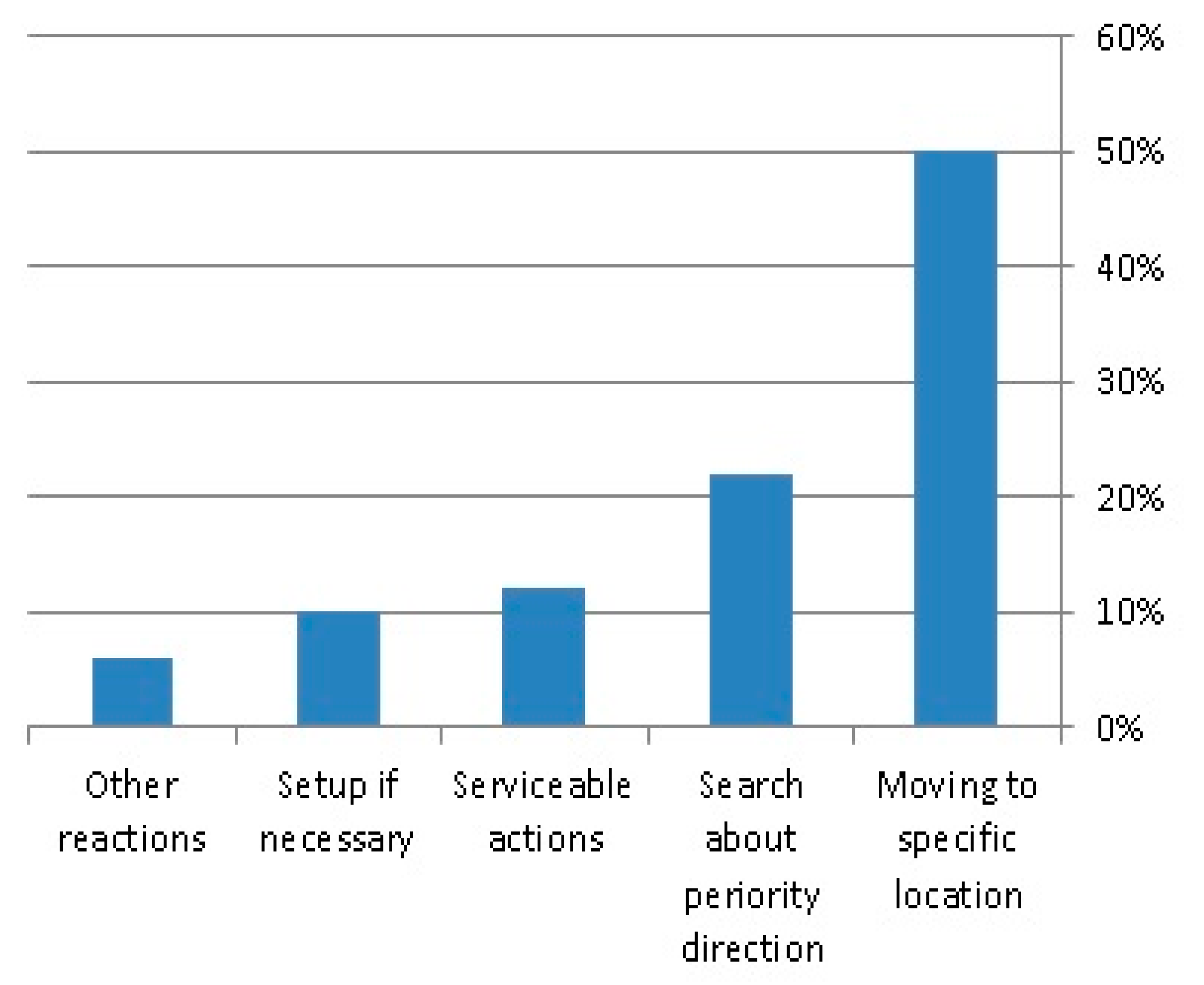
2. Serviceable Sequence Actions for Route Direction

The proposed plan aims to select the minimum route length between main successive locations ψ_i of extensions (such as electrical transformers, water traps, etc.) that are related in terms of the time spent performing each activity, as illustrated in Figure 1. There are five sequences of activities to minimize the route length and time (moving to specific location (i.e., travel), search about priority direction, cost locations, serviceable actions, setup if necessary, and other sudden reactions).

Blair 2013, states that the performance and efficiency of any sequential activities’ plan depends on four tactical decisions [21]: layout design and its selected locations, assignment policy, priority facilities movement and routing policy—these four are a seed for creating the proposed algorithm shown in Figure 3.

The Classification of Proposed systems emphasizes that layout design is one important factor affecting the processes performance and routing distance. It takes n times to finish n (locations); the numbers of trips to serve all locations are equal to the number of locations requested. The factors to be considered in internal layout include: number of locations, length and width of avenue, number and shape of cross avenue and position of main extension source (I/O point). Is there a cross avenue, yes or no? If yes, how many (I/O) locations? Rear and front cross avenue. There are three types of layouts. The first is a parallel avenues case with an I/O-Point located in the middle, the second and third are Vertical Avenues, but the I/O-point is located in the middle and lower left corner to sketch a Flying-V or fishbone. There is another movement direction in ascending order, according to the full-turnover assignment policy (no backtrack), which sorts all locations to be allocated.

There is another vision to switch the proposed plan from A to B. This divides the layout area into zones, which have similar treating proposed procedures, and will be assigned close to each other. However, this vision showed no significant impact on the performance.

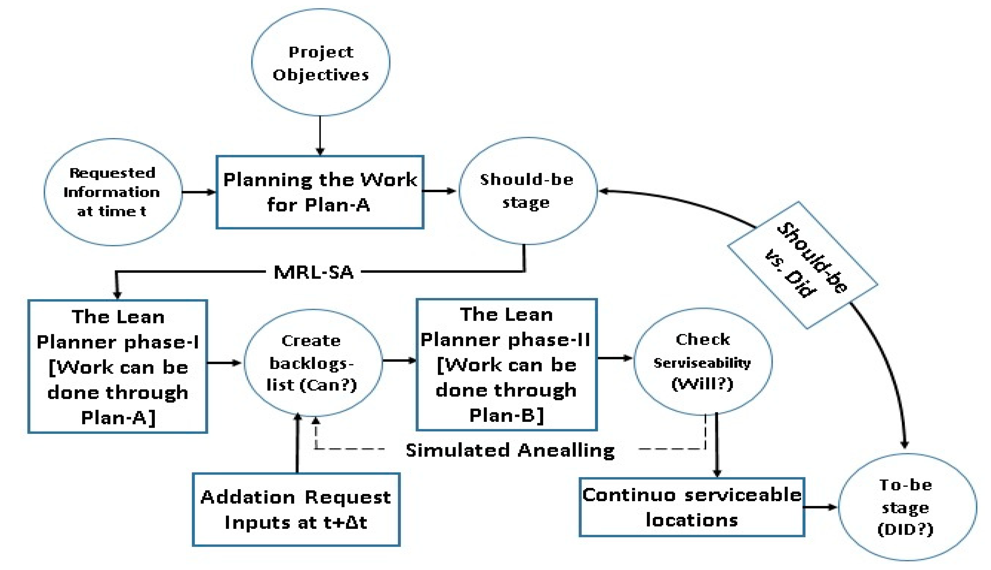
3. Problem Statement in Lean Planner System

The aim of this work is to develop a heuristic algorithm for discovering the shortest route length to serve some locations that lie on a specific layout. The proposed heuristic method aided with SA (MRL-SA) is combined to maximize the number of exchanges in the sequence for the locations in the backlogs-list, as described above. The locations in the backlogs-list have two classifications, unidirectional and bidirectional, which could not support Plan-A/Plan-B when the added locations were not on the proposed routes. Some 185 examples of different locations distribution were generated for unidirectional (i.e., clockwise) and bidirectional (i.e., counterclockwise) movement by choosing interaction values from 1:9 using uniform distribution.

A residential compound contains a large number of building and avenues that need to deploy infrastructure cables and hydrant piping via the sequential procedures list, illustrated in Figure 1, taking into account, the proposed plan created and updated in two aspects, plan-A created according to MRL. In the proposed planning considered in this paper, a contractor faces dynamic stochastic [9] extensions for serviceable items (locations) ${\psi }_i$ through Plan-A (electrical transformers/hydrant pipe or other) and the dynamic stochastic modification of Plan-A to become plan-B ${\psi }_j$ in each period over a finite time horizon. The probability distributions of locations under service, whether at Plan-A or at Plan-B, may be disposed of the specific layout if they are off the route. Only the mean values and the maximum deviations from the mean values can be estimated in each period. The contractor must decide on the number of serviceable items ${\psi }_i$, and if they are serviceable at the beginning of each period t. Once the serviceable items ${\psi }_i$in period t have been observed, the distance to the serviceable items at the end of period t, which is equal to the distance to the serviceable items at the end of period t–1, plus the new distance that belongs to the locations at Plan-A (lpA: location on Plan-A route ${\psi }_i$), and are serviceable in period t less realized $\sum {\mathsf{\psi }}_{\mathrm{i}}$ in period t, is obtained. If there are two choices to select direction when modifying Plan-A ${\psi }_i$to switched to Plan-B ${\psi }_j$, the route length yield to cost analysis, which should be carried out for the proposed change of direction [16], and the route processing cost per item is incurred. If this is neglected and continued to implement Plan-A (i.e., backlogging), costs for items will be added at the end of Plan-A. The contractor can install or dispose the items inserted in Plan-B (lpB ${\psi }_j$) and must decide on the number of items that are (re)serviceable or disposed of at the beginning of each period t + 1. A variable disposal cost per item disposed is incurred when the contractor disposes the items of lpB ${\psi }_i$. Once the lpB items in period t have been observed, the route length to the lpB items at the end of period t—which is equal to the route length of the lpB at the end of period t–1 plus the realized serviceable lpB items in period t, minus the (re)serviceable or disposed items in period t, according to the cost analysis, is obtained. If the ending route length of the (re)serviceable items are in two different directions, a route processing cost per item is incurred (operational cost-saving analysis) to make a decision. Note that the ending route of the (re)serviceable items cannot be negative. Without loss of generality, we assume that serviceable, (re)serviceable and disposable items from Plan-A or Plan-B occur instantaneously through executing Plan-A. In the following, important parameters and decision variables that are used in selecting the route direction after starting at t are given. In order to change the listed locations during the execution of the selected proposed plan, a push to create Plan-B is necessary (i.e., some of the serviceable locations may be added while others may be disposed of through executing Plan-A). The problem assumptions are as follow:

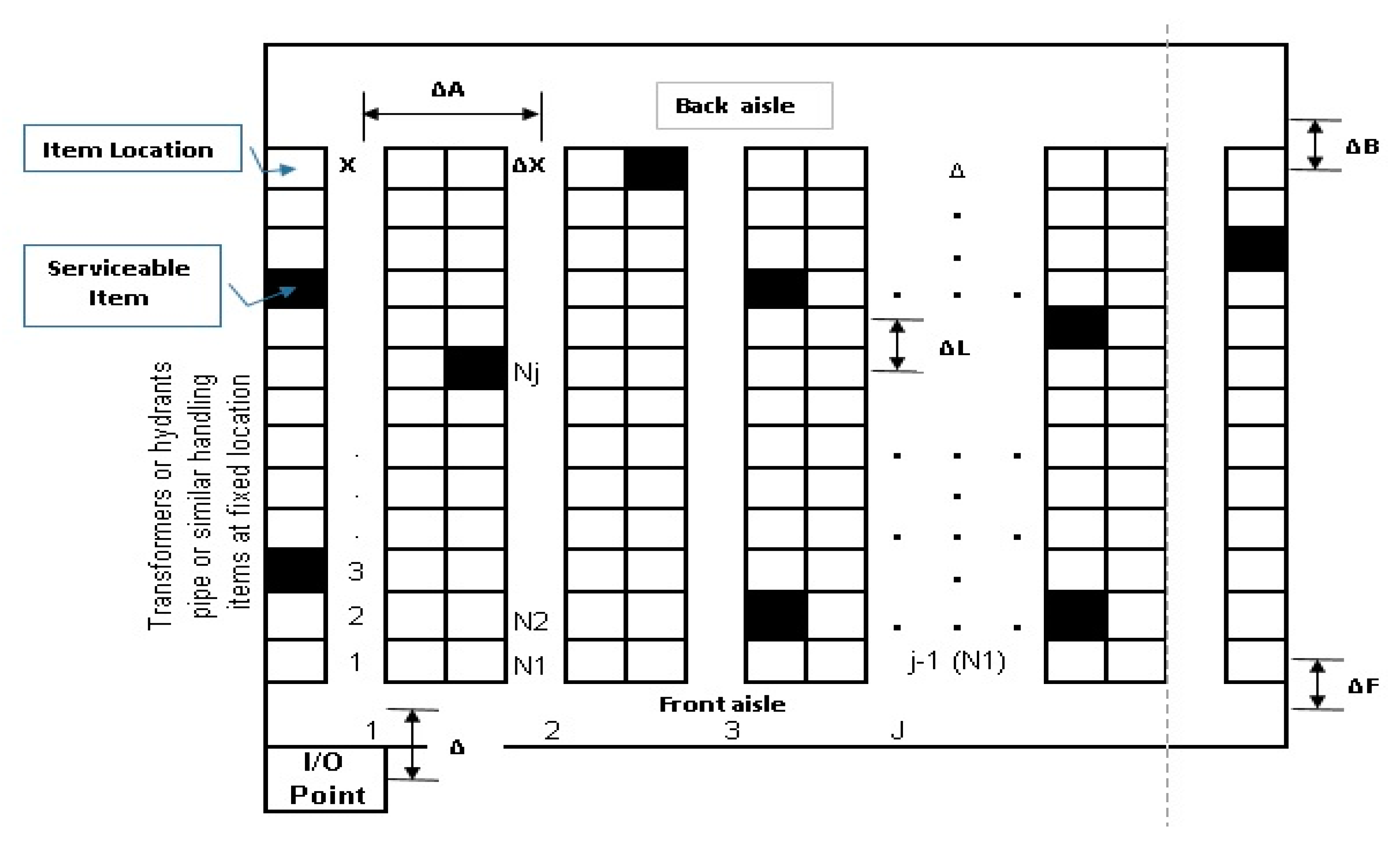
3.1. Structure and Layout

Shape:	Rectangular
Number of blocks:	2 < X < 2000
Main source point location:	Lower left corner
Avenue width:	As OSHA instructed
Service assignment:	Random/proposed
Proposed policy:	Single or groups
Zoning:	None
Proposed system:	Stochastic and dynamic
${\psi }_{i, plan A}$or ${\psi }_{j, plan B}$ Electrical transformers, hydrants valves, etc.

The Layout Assumption

The maximum capability for the study is based on these assumptions. The understudy consists of 2000 locations, J = 40 avenues running between the back and front and N = 100 locations per avenue, each avenue is two-sided and has 100 ${\mathsf{\psi }}_i$ and can be serviceable by being published on each side. For simplicity, the published random assignment policy in this paper deals with locations, not the number of ${\mathsf{\psi }}_i$ in every location vs. the potential bias, which is likely to occur in the location choices cited by Yilun Shang 2019 [22].

3.2. Parameters of Proposed Cost Analysis Plan for Branching Case

If the locations are added for Plan-A to create Plan-B and recalculate the route direction, the first step assumes the method for processing cost analysis to select the minimum cost direction. If the ${\sum }_{cost=0}^{cost=N}{\mathrm{Plan}}_B$, selects Plan-A items ${\mathsf{\psi }}_i$ branches and neglects Plan-B items ${\mathsf{\psi }}_j$to backlogging after finishing all locations in Plan-A proposals ${\mathsf{\psi }}_i$, or applies hybrid modification of items into Plan-B ${\mathsf{\psi }}_j$and adopts its execution according Figure 3.

$C^{PA}:$

Cost of distance drilling (route length) to item ${\mathsf{\psi }}_i$ locations in Plan-A requested.

$C^{PB}:$

Cost of distance drilling (route length) to item ${\mathsf{\psi }}_j$ locations in Plan-B that executes through Plan-A and in its route.

$C^{dpB}:$

Cost of distance drilling for disposing locations ${\mathsf{\psi }}_j$that serviced plan-A or were canceled during Plan-B.

$h^{PA}:$

Item processing cost to serviceable ${\mathsf{\psi }}_i$ at locations in plan-A for requested list L at period t.

$h^{PB}:$

Item processing cost to serviceable ${\mathsf{\psi }}_i$ locations appeared at plan-B, if in the same proposed route.

$b:$

Item backlogging cost to serviceable ${\mathsf{\psi }}_j$ locations at plan-B after finishing Plan-A.

$I_0^S:$

Number of locations ${\mathsf{\psi }}_i$ of plan-A at the beginning of the proposed planning horizon at time (t).

$I_0^R:$

Number of locations ${\mathsf{\psi }}_j$ of plan-B at the beginning of the proposed planning horizon at time (t’).

$r_t:$

Uncertain number of ${\mathsf{\psi }}_j$ locations in plan-B and serviceable or hybrid at plan-A in period t + Δt.

${\overline{r}}_t:$

Estimate of the mean number of ${\mathsf{\psi }}_i$ + ${\mathsf{\psi }}_j$ locations updated to serviceable in period t.

${\widehat{r}}_t:$

Maximum deviation from the mean published number of ${\mathsf{\psi }}_i$ locations updated to serviceable in period t.

$d_t:$

Uncertain serviceable locations’ requested for the list L in period t.

${\overline{d}}_t:$

Estimate of the mean requested list L in period t.

${\widehat{d}}_t:$

Maximum deviation from the mean requested list L in period t.

${\tau }_t^d, {\tau }_t^r:$

Maximum number of uncertain requested and uncertain (re)request # of locations (route length) that can simultaneously deviate from their mean (i.e., ${\overline{d}}_t \mathrm{and} {\overline{r}}_t$) until the end of period t.

Decision Variables

$S_t^A:$

# of serviceable ${\mathsf{\psi }}_i$ locations that are distributed in period t of Plan-A.

$S_t^B:$

# of serviceable ${\mathsf{\psi }}_j$ locations at Plan-B that is updated of Plan-A in period t’.

$X_t^D:$

# of disposed items from the list L in period t’ due to cancelation or against cost analysis step and backlogged to end of the route activities.

$I_t^S:$

# of backlogging locations ${\mathsf{\psi }}_{i+j}$ for requested all locations at the end of period t of Plan-A and Plan-B.

3.3. The Contribution of This Study

The question is, how to make a hybrid between different methods to achieve the maximum benefits of the research objective, when implemented through Lean Planner System.

1-.

Proposed new routing heuristic method [23] to avoid demurrage and control those costs.

2-.

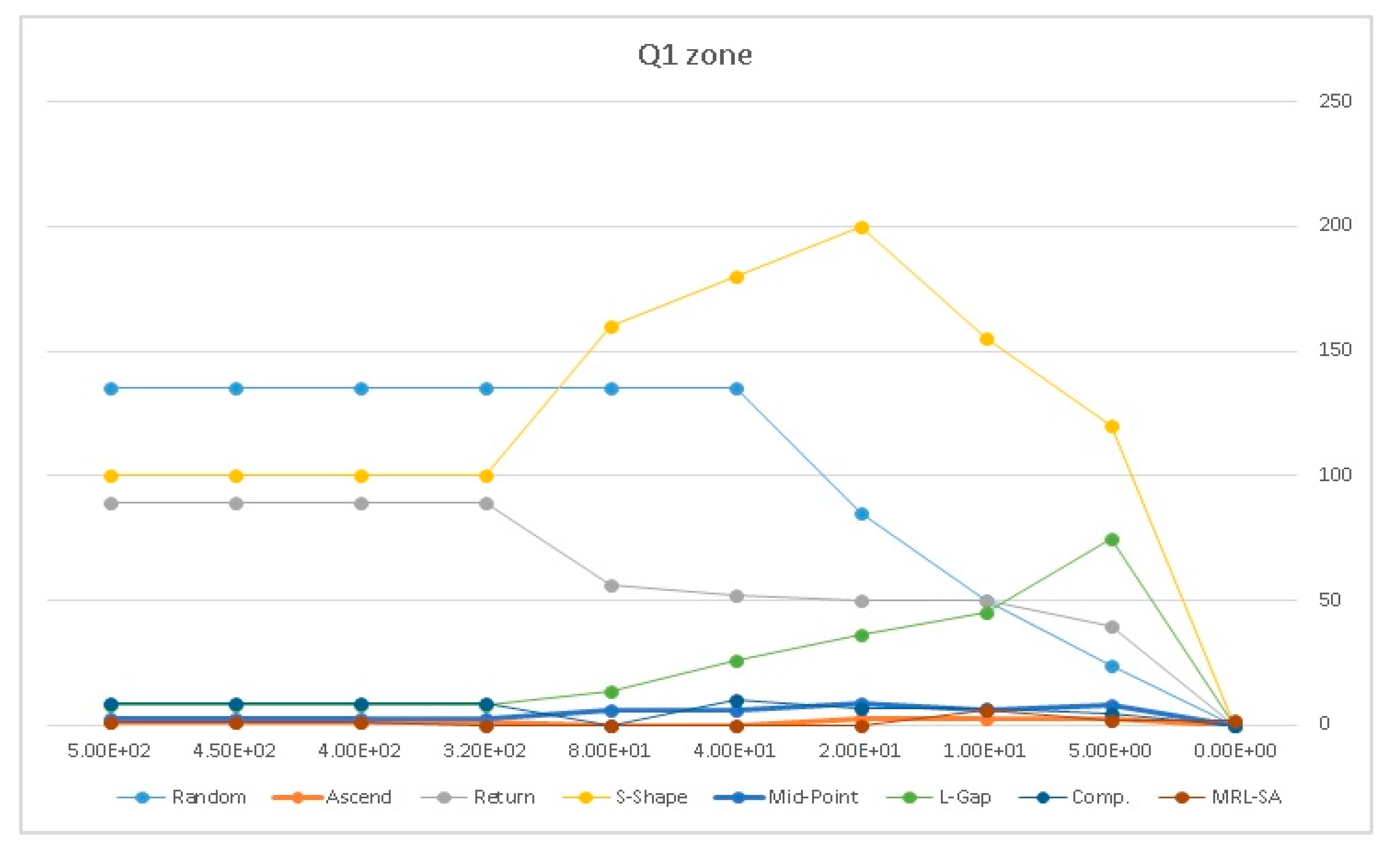
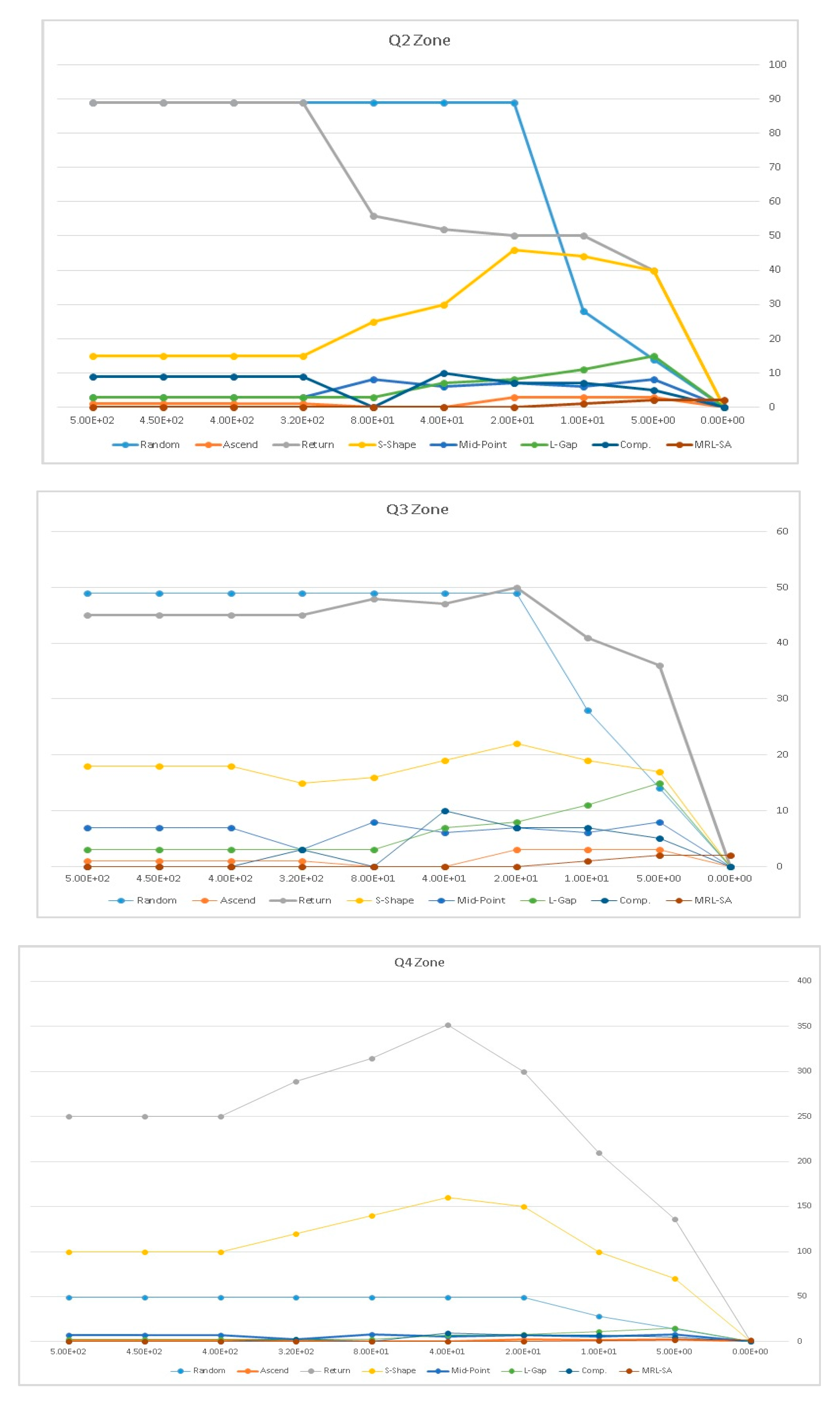
Investigating the impact of proposed regions on the performance of routing heuristics.

The proposed layout consists of: a fixed two dimensional rectangular inside has only one location (J avenue x N two-sided locations per avenue), with one source feeding (I/O-point) located at the extreme lower left corner, as shown in Figure 4. The two end avenues are located near and parallel to the back and front walls of the boundaries. The definition of each symbol on the layout is shown at each location and illustrated in

Table 1. Symbols used in the proposed plan model illustrated in Figure 3.

x, y	Coordinates of serviceable items such as electrical transformers or hydrants or any similar items.	ΔB	The distance between the last ${\mathsf{\psi }}_{\mathrm{i}},{ \mathsf{\psi }}_{\mathrm{j}}$ in the vertical avenue and the back avenue.
j	Avenue number on suggest layout plan	ΔA	The distance between two adjacent avenues.
N	Number of serviceable targeted locations at each avenue whether in Plan A/plan B	Δl	The distance between two adjacent locations: ${\mathsf{\psi }}_{\mathrm{i}},{ \mathsf{\psi }}_{\mathrm{j}}$.
J	Total number of avenues, whether horizontal, vertical, or diagonal	ΔF	The distance between the first location and the front avenue.
i	Number of the location at the avenue where number of locations is (1,2,3…, i, … N)	ΔD	The distance between the feeding/departure point (I/O point) and the front avenue.
${\mathsf{\psi }}_{\mathrm{i}},{ \mathsf{\psi }}_{\mathrm{j}}$	Targeted Location items in plan-A and plan-B	ΔS	The distance between the feeding source point (I/O point) and the point in the straight line of front avenue.
${\delta }_b$	Variable keeps back calculated distance $\sum {\lambda }_i$	L	List of requested locations to be served
		Lb	List of backlogged locations to be served
${\mathit{\lambda }}_{\mathit{i}}$	Route length	${\mathit{\lambda }}_{\mathit{i}}^{\mathit{d}}$	Route length under cost analysis test

.

The locations of the ψ is indicated as (the first location in any avenue j) where jϵ {1,2,…,J} is (j − 1)N + 1, the second location in any avenue j is (j − 1)N + 3, …, (j − 1)N + i where i ϵ {1,2, …,N} and so on, to reach the last location at any avenue j is j_N, but the routing is restarted when ΔS becomes a straight distance back and returns to the same point to start next trip of connection. The distance between any two locations x in j_x and y in j_y is the shortest distance which are calculated as:

• The traversed distance (backtrack), the current avenue to the back avenue, then going to the next serviceable location ${\mathsf{\psi }}_i$.
• The distance if the returned to the front avenue, then going the next serviceable location.

Then follow the minimum distance.

The distance of serviceable all locations in Plan-A is calculated as shown in the next equation [24]:

$$\begin{array}{c}{\mathit{\lambda }}_{\mathit{i}}=\mathit{m}\mathit{i}\mathit{n}{\displaystyle \sum _{\mathit{\psi }=1}^{\mathit{n}}}[∆\mathit{l} \left(2\mathit{N}-{\mathit{i}}_{\mathit{x}}-{\mathit{i}}_{\mathit{y}}\right)+2∆\mathit{B}+\left|{\mathit{j}}_{\mathit{x}}-{\mathit{j}}_{\mathit{y}}\right|∆\mathit{A}+2∆\mathit{D}, ∆\mathit{l}\left({\mathit{i}}_{\mathit{x}}+{\mathit{i}}_{\mathit{y}}-2\right)\\ +2∆\mathit{F}+\left|{\mathit{j}}_{\mathit{x}}-{\mathit{j}}_{\mathit{y}}\right|∆\mathit{A}+2∆\mathit{D}] \end{array}$$

(1)

where:

$$j_x=\left[\frac{x}{N}\right],\dots i_x=x-\left[\frac{x}{N}\right]N,\dots j_y=\left[\frac{y}{N}\right],\dots i_y=y-\left[\frac{y}{N}\right]N$$

3.4. Cost Analysis Formulation

$$\begin{array}{c}{\mathit{\lambda }}_{\mathit{i}}^{\mathit{d}}=\mathit{M}\mathit{i}\mathit{n} {\displaystyle \sum _{\mathit{t}=\mathbf{1}}^{\mathit{T}}}[h^{PB}{\varnothing }_{\mathit{t}\mathit{T}} ({\mathit{I}}_{\mathbf{0}}^{\mathit{R}}+{\displaystyle \sum _{\mathit{i}=\mathbf{1}}^{\mathit{t}}}({\mathit{r}}_{\mathit{i}}-∆B\left({\mathit{P}}_{\mathit{i}}^{\mathit{B}}-{\mathit{P}}_{\mathit{i}}^{\mathit{D}}\right)))+{\mathit{I}}_{\mathit{t}}^{\mathit{S}}+C^{PA}{\mathit{\lambda }}_{\mathit{i}}{S}_t^A+C^{PB}{\mathit{\lambda }}_{\mathit{i}}{\mathit{S}}_{\mathit{t}}^{\mathit{B}}\\ +C^{dpB}{\mathit{X}}_{\mathit{t}}^{\mathit{D}}]+h^{PB}{\mathit{\beta }}_{\mathit{t}}{\tau }_t^r+\mathit{T}{h}^{PB}{\mathit{I}}_{\mathbf{0}}^{\mathit{R}}+{\displaystyle \sum _{\mathit{i}=\mathbf{1}}^{\mathit{t}}}(T-\mathit{t}+\mathbf{1}){\overline{r}}_t\end{array}$$

(2)

$$S_t^A=S_{t0}^A+{{\displaystyle \sum }}_{k=1}^{t-1}\left(d_k{S}_{tk}^{1A}+r_k{S}_{tk}^{2A}\right) 1\le t\le T$$

(3)

$$S_t^B=S_{t0}^B+{{\displaystyle \sum }}_{k=1}^{t-1}\left(d_k{S}_{tk}^{1B}+r_k{S}_{tk}^{2B}\right) 1\le t\le T$$

(4)

$$X_t^D=X_{t0}^D+{{\displaystyle \sum }}_{k=1}^{t-1}\left(d_k{X}_{tk}^{1D}+r_k{X}_{tk}^{2D}\right) 1\le t\le T$$

(5)

$$I_t^S=I_{t0}^S+{{\displaystyle \sum }}_{k=1}^{t-1}\left(d_k{I}_{tk}^{1M}+r_k{I}_{tk}^{2M}\right) 1\le t\le T$$

(6)

Subject to:

$$I_t^S\le h^{PA}\left[I_0^S+{{\displaystyle \sum }}_{i=1}^t(S_i^A+S_i^B-{\overline{d}}_i\right)+q_t{\tau }_t^d+{{\displaystyle \sum }}_{i=1}^t{\vartheta }_{it}] 1\le t\le T, d\in {\lambda }_i^d$$

(7)

$$I_t^S\ge b\left(-I_0^S-{{\displaystyle \sum }}_{i=1}^t(S_i^A+S_i^B-{\overline{d}}_i\right)+q_t{\tau }_t^d+{{\displaystyle \sum }}_{i=1}^t{\vartheta }_{it}] 1\le t\le T, d\in {\lambda }_i^d$$

(8)

$$I_0^R+{{\displaystyle \sum }}_{i=1}^t(r_i-S_i^B-X_i^D)\ge w_t{\tau }_t^d+{{\displaystyle \sum }}_{i=1}^t{\epsilon }_{it}+P_{t+1}^B] 1\le t\le T, d\in R_t$$

(9)

$$S_t^A\ge 0, S_t^B\ge 0, X_t^D\ge 0 1\le t\le T,$$

(10)

$$q_t+{\vartheta }_{it}\ge {\widehat{d}}_i 1\le i\le t\le T$$

(11)

$$w_t+{\epsilon }_{it}\ge {\widehat{r}}_i 1\le i\le t\le T$$

(12)

$${\beta }_T+{\varnothing }_{tT}\le \left(T-t+1\right){\widehat{r}}_{it} 1\le i\le T$$

(13)

$$q_t\ge 0, {\vartheta }_{it}\ge 0, w_t\ge 0, {\epsilon }_{it}\ge 0, {\beta }_{T }\ge 0, {\varnothing }_{tT}\ge 0\dots \dots 1\le i\le t\le T$$

(14)

where

$D_t=\left\{{\overline{d}}_i+{\widehat{d}}_i{z}_i:\left|z_i\right|\le 1\forall 1\le i\le t\right\} and R_t=\left\{{\overline{r}}_i+{\widehat{r}}_i{z}_i:\left|z_i\right|\le 1\forall 1\le i\le t\right\}$ [24].

The objective function (2) is the total test cost in the branch case for a new location added to Plan-A but not on the suggested route, to a serviceable specific location or if disposed. Constraints (7) and (4) keep track of the distance at the end of period t or back locations at the end of period t for any possible realization of ${\psi }_{i+j}$. Note that $I_0^S+{\sum }_{i=1}^t(S_i^A+S_i^B-d_i)$ is the capability level of the service requested ${\psi }_{i+j}$ at the end of period t. Constraints (9) ensure that the capability level is nonnegative at the end of period t. Constraints (10) are for the non-negativity of variables. The variables $q_t, {\vartheta }_{it},w_t,{\epsilon }_{it},{\beta }_{T and }{\varnothing }_{tT}$ for $1\le i\le t\le T$ are used to transform the uncertain model into a traceable model. Next, we show that there are flaws in constraints (9) and (13) of the model, given the above.

To reformulate the model illustrated in (2)–(10) to a traceable model and to control the uncertainty behavior, the right-hand sides of variables $S_t^A, S_t^B, X_t^D, I_t^S$ shown in the proposed cost analysis are in step with constraints (15)–(16). The proposed step inferred, as deduced from Ben-Tal et al. (2004), the following inequality:

$${\alpha }_0+{{\displaystyle \sum }}_{t=1}^T\left({\alpha }_t{a}_t\right)\le 0 \forall a_t\in \left[{\overline{a}}_t-{\widehat{a}}_t, {\overline{a}}_t+{\widehat{a}}_t\right] 1\le t\le T$$

(15)

The constraint (11) represents an uncertain parameter, and ${\alpha }_t$ for $1\le t\le T$ is an expression involving some decision variables, which can equivalently be reformulated as

$${\alpha }_0+{{\displaystyle \sum }}_{t=1}^T\left({\alpha }_t{a}_t+{\gamma }_t{\widehat{a}}_t\right)\le 0 \forall -{\gamma }_t\le a_t\le {\gamma }_t and 1\le t\le T$$

(16)

The proposed step will yield a component-disposal policy that adapts the ${\psi }_{i+j}$ disposal location, based on the realization of requested and updated requests. The ${\psi }_{i+j}$ disposal policy, which will be feasible regardless of the realization of requested and updated requests, is determined by the realized ${\psi }_{i+j}$ as requested and updated, and by the values of$S_{t0}^A, S_{tk}^{1A},$ $S_{tk}^{2A}, S_{t0}^B, S_{tk}^{2B}, X_{t0}^D, X_{tk}^{1D}, X_{tk}^{2D}$ variables for $1\le t\le T and for 1\le k\le t-1$, that are found by solving the proposed equations. For example, the number of requests ${\psi }_{i+j}$ that are collected in period 2 (i.e., $S_2^A$) is determined by $S_{20}^A+d_1{S}_{21}^{1A}+$ $r_1{S}_{21}^{2B}$ where $d_1 and r_1$ are the realized ${\psi }_{i+j}$ requested and updated in period 1 respectively, while $S_{20}^A, S_{21}^{1A} and S_{21}^{2B}$ are found by solving the proposed equations at time t₀.

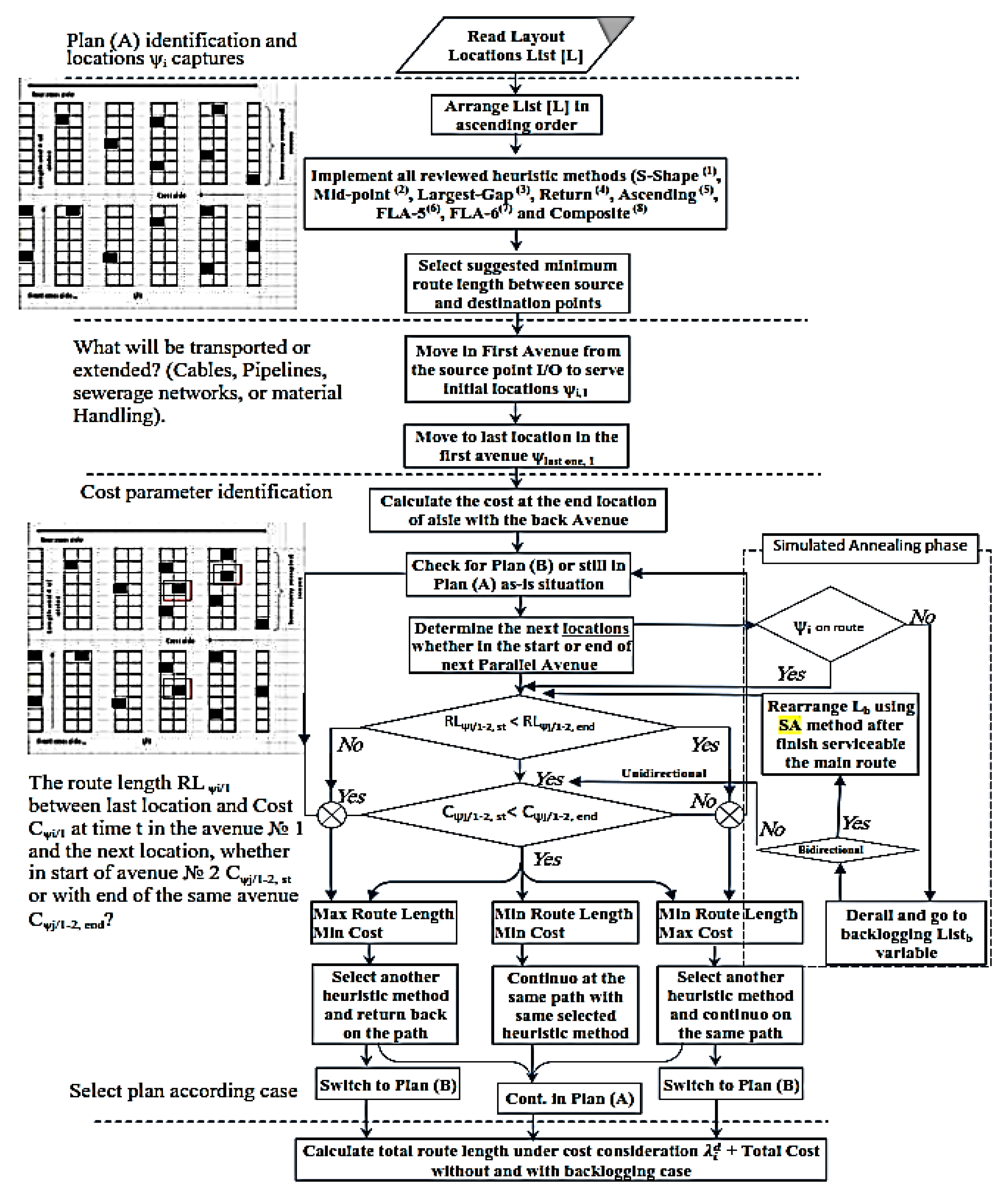
4. Lean Planner System-Phase I [Proposed MRL Heuristic Method]

The minimum route length plan is the main objective of this study. This method has one main drawback, which has a negative impact on its performance. This drawback is that when the route must move from the current avenue to the next one, it just follows the ascending high frequency locations of the ${\psi }_{i+j}$list. To eliminate this drawback, the proposed solution will decide whether to traverse its avenue or return back through the front avenue, based on the shortest routing with minimum cost analysis. The proposed plan has been updated during the connection mission, where some of locations were removed the list and others were returned to the requested list during implementation. The updated ${\psi }_j$ request will be classified to get into Plan-A implementation or disposed, to avoid obstruction or downtime during the implementation mission. This explanation reveals that the problem must be processed as an uncertainty case related to time. The detailed steps of proposed heuristic are as shown in next algorithm.

Step1:	Arrange the requested list L of (Plan-A) according to the serviceable locations ${\mathsf{\psi }}_i$ in an ascending according to specific layout.
Step2:	The route starts from the feeding source point to the first location ${\mathsf{\psi }}_i$ in L
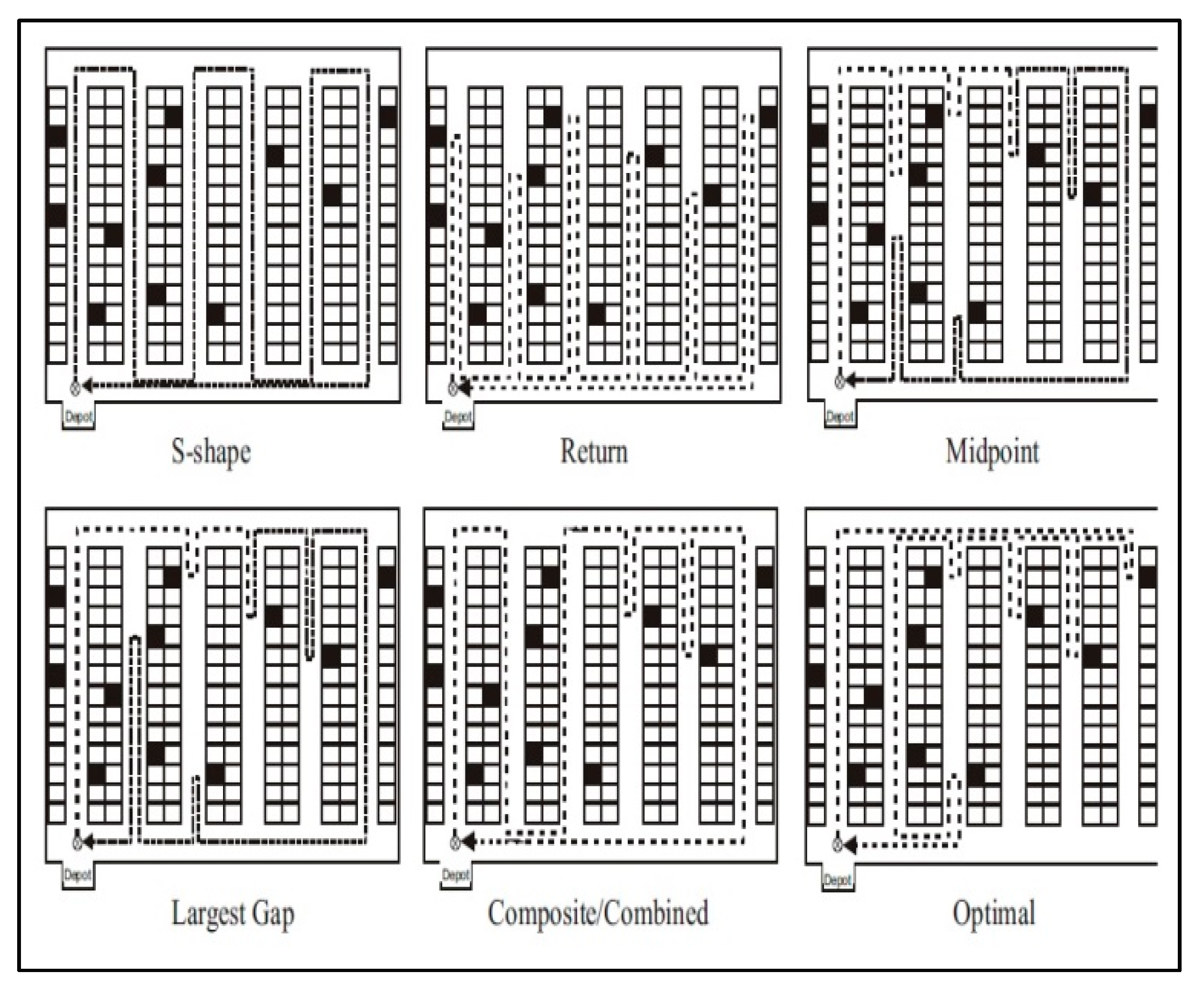
Step3:	The serviceable all ${\mathsf{\psi }}_i$ in (Plan-A) list is subject to one of previous published methods (such as: S-Shape, Mid-point, Return, L-Gap, Return, Composite or Ascending) and uses the same method that have minimum route to service ${\mathsf{\psi }}_j$ in (Plan-B) that id in the same proposed direction and stops at the last one ${\mathsf{\psi }}_{i+j}$ in the last avenue, then goes to step 10.
Step4:	Resolve serviceable ${\mathsf{\psi }}_j$ (which are on the proposed route) items in (Plan-B) and considers last ${\mathsf{\psi }}_i$ is the starting point, and keeps the previous calculated distance route in variable ${\mathsf{\delta }}_b=\sum {\lambda }_i$ via the same published method stated in step 3.
Step5:	If there are ${\mathsf{\psi }}_j$ not on the proposed route, a backlogs list is created for them
Step6:	${\lambda }_{im}$ is the distance between the current location I and m, where m is the first serviceable location in the next avenue, according to the list L of (Plan-A). ${\lambda }_{jn}$ is the distance between the current location j and n, where n is the last serviceable location in the next avenue, according to the list L of (Plan-B), which is based on resolving the new distribution of serviceable ${\mathsf{\psi }}_{i+j}$ on the same route.
Step7:	If the ${\mathsf{\psi }}_j$ is not on the (Plan-A) route, and needs to reverse its direction, it must be subject to the step 7 analysis.
Step8:	If ${\sum }_{cost=0}^{cost=N}{\mathrm{Plan}}_{\mathrm{A}}\le {\sum }_{cost=0}^{cost=N}{\mathrm{Plan}}_B$, select (Plan-A) items ${\mathsf{\psi }}_i$ branch and neglect (Plan B) items ${\mathsf{\psi }}_j$to backlogging after completing all (Plan-A) proposal items ${\mathsf{\psi }}_i$, or carry out hybrid modification of items into (Plan-B) ${\mathsf{\psi }}_j$ and merge the suggested routes.
Step9:	If min [(${\lambda }_{im}$ > ${\lambda }_{jn}$+ $∆F$)] < y, reverse the sequence of the next avenue in list L.
Step10:	Continue serviceable the next item in L, then go to step 3 again.
Step11:	Go back to the front avenue, then go to the feeding source point.

4.1. Performance Measure

The performance is a measurable response that leads to an understanding of efficiency and effectiveness (checking and handling the location right), which is important to determine the total route distance$\sum {\lambda }_i^d$, which is required for the service of all ψ and make a comparison with the minimum route, according to the published methods, and uses the deviation $\%D{v}_{\propto }=\frac{{\lambda }_i^d{}_{\propto }-min{\lambda }_i^d{}_{\propto }}{min{\lambda }_i^d{}_{\propto }}\times 100$, where it represents the percentage of deviation for the suggested route distance $\propto$ from the minimum routing distance, and $\sum {\lambda }_i^d{}_{\propto }$ is the total distance of the routing heuristic $\propto .$

4.2. Illustrative Example for implementing MRL-SA (${\psi }_i$ Distribution)

This example explains how the route distance is calculated based on the MRL-SA heuristic, assuming the compound have five avenues, each of which have 16 two-sided building locations, and the feeding source point is located at lower extreme left corner, and the black cells are the locations of ψ_i to be serviced, as shown in Figure 5. The requested list L is required for serviceable locations # as follows (80, 67, 16, 29, 54, 84, 75, 23, 19, 8, 50, and 12) at period t for Plan-A and 1, 2, 4, 5, 6, 7, 41, 63, at period t’ for Plan-B. Where, ($∆F=∆B=1 unit, ∆A=3 units, ∆D=0 unit, ∆l=1 unit)$, by applying the distance equations, which are described above. During the implementation according to time, the ${\mathsf{\psi }}_{41, 63}$ is located on the proposed route, and therefore will serviceable according to the cost and distance analysis, but other added locations shall be saved in the backlogs list L_b. The proposed MRL-SA tackles L_b via the simulated annealing method after arriving at the end location in the proposed route.

4.2.1. Lean Planner System—Phase-I: Route Based on the Proposed MRL Heuristic

The following are the applied steps of algorithm on the example:

Step1: 

Arrange the locations ${\psi }_i$list in an ascending order L = (3, 8, 12, 16, 19, 23, 29, 45, 50, 54, 67, 75, 80, 84)

Step2: 

The plan aims to go from the feeding source point to the location ${\psi }_3$ (the distance ${\lambda }_i$ = 3 units)

Step3: 

The plan aims to service all ${\psi }_i$ in the current avenue, and stop at the last ${\psi }_{16}$ in the same avenue in this illustrative example (the distance${\lambda }_i$ = 3 + 5 + 4 + 4 = 16 units).

Step4: 

Calculates the distance between the location (${\psi }_{16}$, ${\psi }_{19}$), which is 20 units, and (${\psi }_{16}$, ${\psi }_{29}$), which is 10 units to arrive at the same location (Plan-A). [Take into account costs analysis equations]

Step5: 

The direction will reverse locations in this avenue because 10 < 20, and go to location ${\psi }_{29}$ (the total distance ${\lambda }_i$= 16 + 10 = 26 units).

Step6: 

The proposed plan will collect ${\psi }_i$ from locations ${\psi }_{29}$, ${\psi }_{23}$, ${\psi }_{19}$ and the total travelling distance at end of this avenue is ${\lambda }_i$= 16 + 10 = 26 units.

Step7: 

At t’, the location ${\psi }_{41}$ is added to the layout and placed on the track route. Therefore, there is no need to use cost analysis equations and continue with the MRL method.

Step8: 

Calculates the distance between locations (${\psi }_{19}$, ${\psi }_{41}$), which is 11 units, while the distance between (${\psi }_{19}$, ${\psi }_{50}$) is 20 units. [Take into account costs analysis equations]

Step9: 

The track route will follow the ascending arrangement and go to location 4, because 11< 20. Therefore, the travelling distance ${\lambda }_i$= 37 + 11 = 48 units.

Step10: 

The track route will collect ${\psi }_i$ from the locations ${\psi }_{41}$, ${\psi }_{45}$, ${\psi }_{50}$ and continue on route (the total distance ${\lambda }_i$= 48 + 4 + 5 = 57 units).

Step11: 

Calculates the distance between locations (${\psi }_{50}$, ${\psi }_{54}$), which is 21 units, while (${\psi }_{50}$, ${\psi }_{67}$) is only six units. [Take into account costs analysis equations]

Step12: 

The direction will reverse the ascending arrangement, because 6<21, and go to location ${\psi }_{67}$ (the route distance ${\lambda }_{i }$= 57 + 6 = 63 units).

Step13: 

At t’, location ${\psi }_{63}$ is added to layout (Plan B), but not effects on direction because it between two terminal locations (${\psi }_{54}$, ${\psi }_{67}$). Therefore, this location will be serviced on the track route.

Step14: 

The proposed route will serve locations ${\psi }_{67}$, ${\psi }_{63}$, ${\psi }_{54}$, and the route distance will reach ${\lambda }_i$= 65 + 4 + 9 = 78 units.

Step15: 

Calculates the distance between the locations (${\psi }_{54}$, ${\psi }_{75}$), which is 12 units, while (${\psi }_{54}$, ${\psi }_{84}$) is 19 units. [Take into account costs analysis equations]

Step16: 

The route will follow the ascending arrangement, because 12 < 19, and go to location ${\psi }_{75}$. Therefore, the route distance ${\lambda }_i$= 78 + 13 = 91 units.

Step17: 

The proposed plan will collect ${\psi }_i$ from locations ${\psi }_{75}$, ${\psi }_{80}$, ${\psi }_{84}$ and the total route distance ${\lambda }_i$= 91 + 5 + 4 = 100 units.

Step18: 

The proposed route direction will return to the front avenue and back to the main upstream source distance ${\lambda }_i$= 100 + 16 = 116 units.

Step19: 

The proposed route will return to the feeding source point and the route distance ${\lambda }_i$= 116 + 12 = 128 units.

This solution is done via implementing MRL (i.e., Plan-A), and create a backlog-list for evolving mandates for new locations (Plan-B), which will tackle by Simulated Annealing SA to enhance the solution.

4.2.2. Lean Planner System Phase-II: Backlogs List Tackling Via SA

The optimum sequence for the backlogs list was obtained for both the bidirectional and unidirectional route. In this work, a seed sequence layout route was obtained by MRL (i.e., based on hybridizing superiority heuristic methods). The SA method increases the performance of implementation by finding out the best sequence of backlogs list locations by computing the objective value, as given below. Plan-B, modifies Plan-A at t’ by inserting new locations ψ_i, before and after the proposed method starts at time t, which the backlogs list tackles via SA and rearranges the locations ψ_j randomly, then measures the route length and related cost, then adds that to the previous data obtained by MRL.

In this work, the initial temperature of 500 °C was chosen via expert. The solution can be accepted with an associated probability of 0.92, when it was inferior by 60%, relative to the original solution (expected by proposed heuristic method). Therefore, the initial setting was followed as given below:

P = exp ($-{\lambda }_i^{∆}$/T), i.e., 0.92 = exp(−60/T) or T = 500 °C, Then the SA algorithm starts at a temperature of 500 °C, with temperature reduction factor of 0.92. In this work, the numbers of temperature stages were taken as 42. Then the final temperature was, T_f = 500 * (0.92)⁴² = 20 °C.

The initial seed sequence appeared during implementing Plan-A or a serviceable Plan-B on route were 2-1-6-3-4-7-5, according to t’. If the initial temperature = 500 °C, ACCEPT = 0 and TOTAL = 0 are set as 12 different sequences from the initial backlogs list sequence. Objective values for the 12 sequences were computed, and Δ length/unit (i.e., double the distance between the objective and real route length) were calculated as shown in

Table 2. Different sequences and objective values for bidirectional path flow.

Simulated Annealing Steps Technique	S.No.	SA Sequences							Objective Values	Δ Length/unit	Δ Cost^3
1. Take an initial solution of S from implementing published heuristic method and choose the least value	1	1	6	3	2	4	7	5	42	−6	−1.6
2.  Set an initial temperature, T > 0	2	2	6	1	3	4	7	5	42	−6	−1.6
3.  While not frozen do the following:	3	2	1	3	6	4	7	5	40	−10	−1
3.1 serviceable all locations ψi at the following L list every avenue:	4	2	1	6	4	3	7	5	36	−18	−1.6
3.1.1 allow to enter new locations ψj	5	1	2	6	3	4	5	7	38	−14	−1.4
3.1.2 Sample backlogs at S’	6	2	1	6	3	4	5	7	43	−4	−0.4
3.1.3 Let ∆ = S’-S	7	1	2	6	3	4	7	5	42	−6	−0.6
3.1.4 If ∆ ≤ 0	8	6	2	1	3	4	7	5	40	−10	−1
Then set S ≤ S’	9	2	3	1	6	4	5	7	41	−8	−0.8
else set S← S’ with a probability of exp (-∆/t)	10	4	2	1	6	3	7	5	37	−16	−1.6
3.2 Set T = r*T, where r is the reduction factor.	11	2	7	1	6	3	4	5	36	−20	−1.9
4. Return S.	12	5	2	1	6	3	7	4	40	−10	−1

.

Among the twelve Δ route length/unit, −20 was the least value, its corresponding sequence was taken as preferred sequence 2-7-1-6-3-4-5, its objective value was 36, and the TOTAL and ACCEPT increased by one.

5. MRL-SA Verification

This section focuses on analyzing the results of the 185 different implemented distributions of different locations for all the published methods that are compared with proposed heuristic, to find a relationship between them and a similarity level to create verification level for the proposed method. Also, the objectives of the enterprises were collected according to a generic framework [25] using five-point Likert scales, which revealed four independent variables as Losses cost, route length, traveling time and processing time.

Table 3. Reviewed and Proposed heuristics implementation (statistical analysis ×10³).

No.	Heuristic Methods	N	Mini. ${\mathit{\lambda }}_{\mathit{i}}^{\mathit{d}}$	Max. ${\mathit{\lambda }}_{\mathit{i}}^{\mathit{d}}$	∑ Route	SD
1	S-Shape CW	185	3.45	4.62	4.068448	0.302306
2	S-Shape CCW	185	4.13	5	4.673793	0.249862
3	Flow Line Analysis FLA-5	185	2.97	4.54	3.816207	0.438494
4	Mid-point, CCW	185	3.56	4.7	4.222586	0.333508
5	Largest Gap, CW	185	2.65	4.44	3.825	0.436466
6	Largest Gap, CCW	185	3.55	5	4.525	0.363131
7	Return, CW	185	3.08	4.24	3.747931	0.329134
8	Flow Line Analysis FLA-6	185	4.22	5.2	4.881034	0.204302
9	Composite CW	185	3.58	5	4.627931	0.394616
10	Ascending, CW	185	1.81	5	3.82	0.924127
11	Ascending, CCW	185	3.47	4.89	4.065862	0.304677
12	MRL-SA	185	2.65	4.5	3.782759	0.1501061
The obvious outcomes
13	Losses cost	185	3.45	4.9	4.544828	0.205
14	Route length	185	3.65	4.9	4.49569	0.402
15	Traveling time	185	3.045	4.74	4.209052	0.518
16	processing time	185	2.3	4.4	3.691954	0.562

illustrates that from a total of 2000 examples for different 28 enterprises, the sample sizes of 185 different random distributions were chosen, as cited in Israel Glenn 1992, using the Taro Yamane formula. The simulation intervals were 108, with a mean route of 45.72 units (SD = 12.79, range 22–60 unit length) and 77, with a mean route of 32.02 units (SD = 8.65, range 22–54 unit length). Descriptive statistics are shown in Table 3 (i.e., the means and standard deviations of different heuristics), and was found to be 4.54 (S.D = 0.205), 4.49 (0.402), 4.21 (0.0518) and 3.69 (0.562), respectively, for enterprises objectives. The frequencies were calculated to test the normality of data and it was found that the data used in present research were normally distributed. Select the value above average in the minimum or maximum columns, and the minimum standard deviation is less than the average and maximum mean. The impact factors of measurement objectives illustrated in

Table 4. The impact factors of measurement objectives.

Effect on (Influence)		Losses Cost		Route Length		Traveling Time		Processes Time
Is These Methods	Objectives Profile	Reduce Disposal	Backlogging	Satisfaction Case	Supplement and Drilling	Avoid Demurrage	Enhancing Reputation	Reliability	Downtime	Over Processing		Effective Profile λi (0.562)		Measured Impact Profile μi (0.35311)
Affected by		c.1.	c.2.	c.3.	c.4.	c.5.	c.6.	c.7.	c.8.	c.9.	Objectives Weight
S-Shape CW	3.1	3	5	3	4	4	3	ϕ	ϕ	ϕ	88.06	3.74	80.36	3.41
Mid-point, CCW	3.8	3	3	2	4	2	3	4	2	4	69.89	2.97	85.88	3.65
Flow Line Analysis FLA-5	4.1	4	3	3	2	5	2	3	5	ϕ	113.65	4.83	99.05	4.21
S-Shape CCW	3.9	5	4	4	3	3	3	3	4	3	83.77	3.56	106.17	4.51
Largest Gap, CW	3.6	5	4	4	5	2	2	3	3	5	93.08	3.95	82.7	3.51
Largest Gap, CCW	3.8	3	4	4	3	3	3	3	3	ϕ	64.59	2.74	93.37	3.96
MRL-SA	4.3	4	2	4	4	3	5	4	3	3	74.98	3.18	92.47	3.93
Composite CW	5	4	4	4	4	4	4	4	4	5	99.27	4.22	116.56	4.95
Flow Line Analysis FLA-6	3.6	5	3	4	3	3	4	3	3	ϕ	117.75	2.74	86.87	3.69
Composite CCW	4.1	3	3	5	4	3	4	4	2	3	43.99	1.87	99.87	4.24
Ascending, CW	3.9	2	3	ϕ	5	4	4	5	3	5	81.65	3.47	94.46	4.01
Return, CW	3.6	3	1	3	4	4	4	3	3	ϕ	64.5	5	83.56	3.55
Losses cost		195.5	139.4	130.6	154.5	124.6	113.3	89.6	103.3	78.2
Traveling distance^1000 units		5	3.6	3.3	4	3.19	2.9	2.3	2.6	2
Traveling time		−34.2	3.2	−26.7	−26.7	−25	−56.6	−63.6	−28.4	−29.2	0.562
Proposed time		4.6	4.1	4.5	5	4.27	4.8	4.4	3.8	3.1

which prelude to correlation which emerge the hybridization level via correlation analysis which discussed in

Table 5. The hybrid method correlation performance.

	Mid-Point, CCW	FLA-6	S-Shape CCW	Largest Gap, CW	Composite CW	FLA-5	Largest Gap, CCW	MRL-SA	Composite CCW	Ascending, CW	Return, CW
S-Shape CW		0.267	−0.084	−0.066	0.507	−0.209	−0.701	0.418	0.463	−0.226	0.308
Mid-point, CCW			−0.279		−0.423	0.167	0.655	−0.423	−0.144	0.693	−0.311
FLA-6	−0.696				0.7	−0.348	−0.627	0.7	0.075	−0.286	0.685
S-Shape CCW	−0.164	0.057				0.491	−0.286	0.473	−0.52	−0.661	−0.215
Largest Gap, CW	−0.471	−0.739	0.501		−0.499	0.707	0.154	−0.2	−0.306	−0.102	−0.488
Composite CW			0.162			−0.212	−0.67	0.799	0.305	−0.409	0.606
FLA-5							0	0.212		−0.346	0.104
Largest Gap, CCW								−0.67	−0.094	0.529	−0.52
MRL-SA									0.214	−0.574	0.672
Composite CCW										−0.125
Ascending, CW											−0.06
Return, CW									0.478

. Table 5 illustrates the effective of Composite method. Therefore, this work interests with compare the results of many examples between MRL-SA and Composite as illustrate in

Table 6. Comparison of the proposed MRL-SA with less deviation than the composite method at the backlogging case using Lean Planner System phases.

					Comp.		MRL-SA							Comp.		MRL-SA
#b	σ	dt	rt	Imp%	Average	Standard Dev.	Average	Standard Dev.	#b	σ	dt	rt	Imp%	Average	Standard Dev.	Average	Standard Dev.
3	2	18	14	51.5	5121.1	648.4	2482.2	24.4	5	2	18	14	53	5464.5	632.3	2569.3	16.3
3	2	18	16	52.4	5012.7	592.8	2342.8	26.3	5	2	18	16	52.7	5209.6	588	2465.2	22.7
3	2	18	18	52.9	4971.8	510	2342.8	23.2	5	2	18	18	54.6	5295.5	609.7	2402.7	28.5
3	2	20	14	49.4	5439.6	523.3	2754.3	19.3	5	2	20	14	49.4	5539.5	532	2802.2	18.9
3	2	20	16	50.3	5378.3	584	2671	19.1	5	2	20	16	50.4	5475.5	569.1	2714.9	16.3
3	2	20	18	51.2	5248.1	591.3	2562.3	23.5	5	2	20	18	51.4	5392	606.7	2620.3	23.6
3	2	22	14	48.2	5698.3	630	2953.4	31.4	5	2	22	14	50	5901.3	547.9	2950.2	26.3
3	2	22	16	48.1	5633.5	532.5	2926.3	25	5	2	22	16	48.8	5798.9	588.4	2971.8	21.3
3	2	22	18	49.2	5537	600.6	2811.3	24.6	5	4	22	18	50.1	5779.6	549	2884.7	23.1
3	4	18	14	58.1	8569	1145.4	3592.7	75.1	5	4	18	14	59.1	8912.3	1163.6	3645.7	67.1
3	4	18	16	59.4	8670	960.5	3523.8	70.4	5	4	18	16	59.6	8857.2	1088	3577.9	76.3
3	4	18	18	59.5	8222.7	1035.2	3329.3	77	5	4	18	18	60.8	8844	1042.7	3469.4	74.6
3	4	20	14	58.7	9093.1	964.4	3756.3	73.8	5	4	20	14	59	9404.5	1212.4	3857.5	61.8
3	4	20	16	58.4	8773.2	1056.2	3649	60.4	5	4	20	16	58.5	9083.6	1096.2	3773.5	69.2
3	4	20	18	59	8653	1082.9	3548.8	63.7	5	4	20	18	59.6	9028.6	1205.5	3644.7	65.6
3	4	22	14	56.8	9173.6	1103.5	3963.5	60.6	5	4	22	14	57.4	9505.5	1038	4044.8	44.8
3	4	22	16	57.3	9008.5	1143	3848.7	53.3	5	4	22	16	57.6	9296.4	1176.8	3942.7	50.1
3	4	22	18	58.3	8933.6	1094	3726.5	61.2	5	2	22	18	58	9132.1	1229	3835.2	53.4
4	2	18	14	51.8	5277.9	603.7	2543.2	17	6	2	18	14	52.2	5389.6	662.6	2573.8	16.6
4	2	18	16	51.5	5066.4	532	2457.8	21.9	6	2	18	16	54.2	5399.4	624.2	2471	19.8
4	2	18	18	52.6	4998.4	625.1	2368	25.8	6	2	18	18	53.3	5167.9	631.3	2412.9	25.3
4	2	20	14	48.8	5498.3	576.7	2814.8	16.6	6	2	20	14	49.8	5586.9	570.8	2807.3	21.5
4	2	20	16	49.5	5343.2	520.8	2697.8	18	6	2	20	16	51.7	5626.9	600.1	2716.4	19.9
4	2	20	18	50.4	5262	537.7	2609.4	19.7	6	2	20	18	51.6	5474.8	638.1	2650.5	23.4
4	2	22	14	48.6	5764.7	566.4	2960.4	25.2	6	2	22	14	50.6	6062.4	590.5	2996.5	28.2
4	2	22	16	47.8	5686.9	600.1	2969.5	16	6	2	22	16	49.7	5900	564.4	2968.6	20.9
4	2	22	18	48.6	5551.5	575.6	2851.1	18.5	6	4	22	18	50.3	5798.6	618.7	2879.2	19.3
4	4	18	14	59.4	8868.4	1074.1	3610.7	75.8	6	4	18	14	59.8	9213.1	1171.4	3705.3	68.3
4	4	18	16	59.2	8750.2	1117.4	3566.9	65.9	6	4	18	16	60.9	9202.5	1107.5	3602	77.5
4	4	18	18	59.4	8583.1	1183.6	3481.6	69.3	6	4	18	18	60.9	8900.1	1263	3477.1	81
4	4	20	14	58.6	9270.4	1144.3	3834.2	54.4	6	4	20	14	59.2	9478.6	1236.9	3868	63.1
4	4	20	16	57.7	8917.1	1093.1	3768	57.5	6	4	20	16	59.7	9293.8	1181.2	3749	63.6
4	4	20	18	59.7	9041.8	1241	3648.3	52.1	6	4	20	18	59.8	9205	1114.9	3696.7	59.7
4	4	22	14	56.3	9252.7	1109.8	4042.3	50.6	6	4	22	14	57.2	9507.2	1207.6	4068.3	47.5
4	4	22	16	57.9	9335.4	1210.8	3927.2	49.5	6	4	22	16	59.6	9770.2	1127.3	3949.7	58.1
4	4	22	18	59.3	9420.8	1044.5	3830.7	44.9	6	4	22	18	58.5	9304.7	1088.6	3863.4	53.2

.

In this work, two heuristic search algorithms, one combining MRL with SA, and the other combining composite with SA, which was selected from a previous correlation test, were proposed and compared together, and the result of the comparison is illustrated in Table 6.

If the relationship between Plan-A and Plan-B is positive according to impacted deployment shown in Table 4 (as A improved or was implemented in minimum time, B also improved in a vice versa negative relationship), the magnitude of Cor(A, B) measures the strength of the relationship. The closer Cor(A, B) is to 1 or -1 and the sign indicates the direction of the relationship. If the Cor(A, B) > 0, this implies that B and A are positively related. Conversely, Cor(B, A) < 0 implies they are negatively related. If p-value (p < 0.0001) is much less than α = 0.05, this indicates a very high significance. In this table, we analyzed the four types of enterprise needs separately to clarify their affect independently, as illustrated in Table 5.

Thirty-seven sets of input data were generated from the uniform distribution from one to nine for the unidirectional flow path, as well as the bidirectional flow paths [8]. The above combination of the selected heuristic method and the simulated annealing method was tested in the 185 sets of generated data.

Computational Verification Results

The computational results are presented as follows, based on ANOVA and statistical analysis shown in

Table 7. Statistical analysis.

	Ascend	MRL-SA	Return	L-Gap	Mid-point	S-Shape	Comp.
Count	270	270	270	270	270	270	270
Sum	10629.34	1723.28	17541.7	6388.035	7177.268	5186.399	2790.102
Average	39.368	6.383	64.969	23.66	23.5824	19.20889	10.33371
Variance	841.66	90.1069	548.7855	605.4917	924.444	691.3697	189.5498

and

Table 8. ANOVA for upper and lower sectors comparison.

Source of Variation	SS	df	MS	F	p-Value	F Crit
Sample	200566.1	8	25070.77	247.6	8.00*10^−285	1.944
Columns	639676.2	6	106612.7	1053	0	2.105
Interaction	661237	48	13775.77	136.1	0	1.368
Within	184985.9	1827	101.2512
Total	1686470	1886

for measuring the different impacts on the performance of the routing technique if the layout to the parallel sectors such as upper/lower or right/middle/left, is divided. Figure 6 illustrates the average percentage deviation of each routing. It is noticeable that the best routing is MRL-SA without considering the requested size for every location, while Figure 7 shows the interaction between the routing policies by changing the requested locations and controlling the number of ${\psi }_i$ (i.e., until 1300 locations in the layout) at a specific time related to the other locations, according to the published plan. Figure 7 illustrates that the largest gap is best at low duty ${\psi }_i$ until a 4% modification of Plan-A, whether MRL is better than others if it has more than 160 locations from 1300. This value push to improve the proposed heuristic published plan divides into two areas, the upper half, which consists of regions (C, G, K, D, H, L), and the lower half, which consists of regions (A, E, I, B, F, J) and three vertical areas, as shown in

Table 9. Number of locations according to regions classification.

	Requested Area	# of Regions	Regions	# of ${\mathit{\psi }}_{\mathit{i}}$ Locations
1	Upper half	6	C,D,G,H,K,L	1000
	Lower half	6	A,B,E,F,I,J	1000
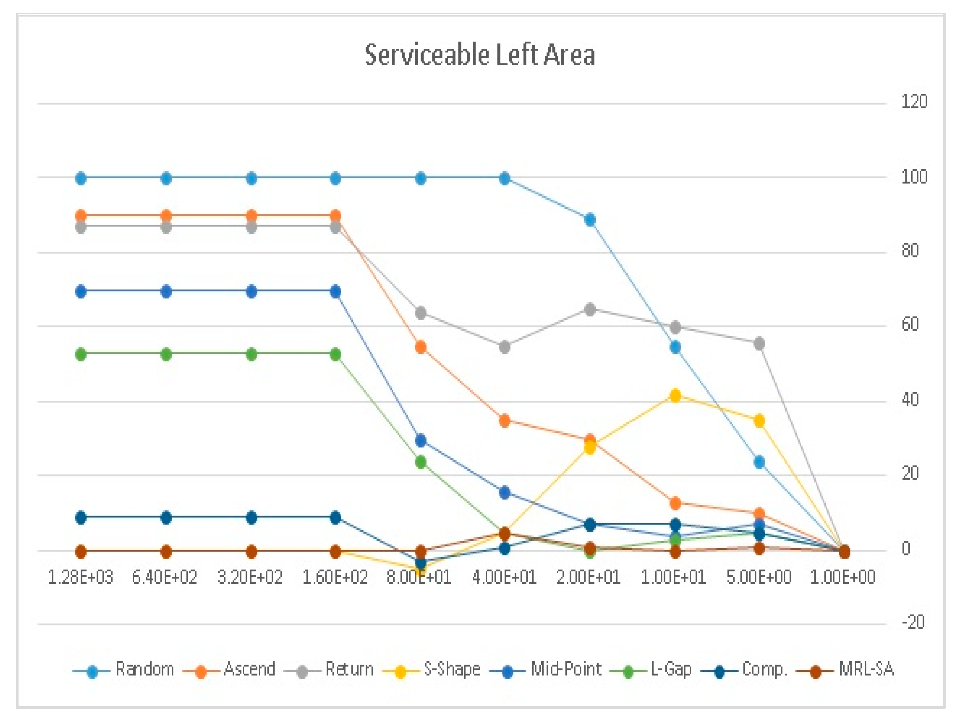
2	Left area	4	A,B,C,D	350
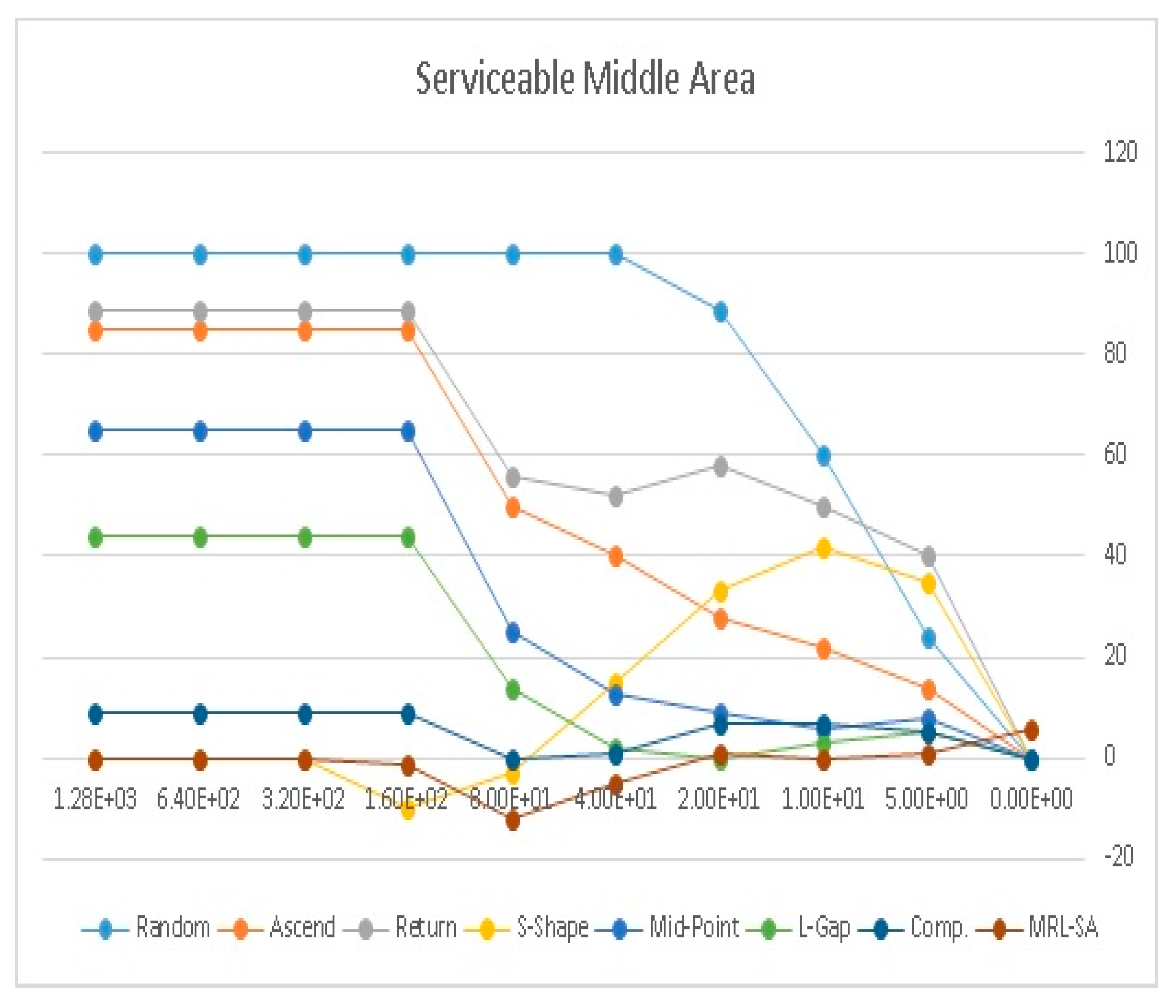
	Middle area	4	E,F,G,H	1300
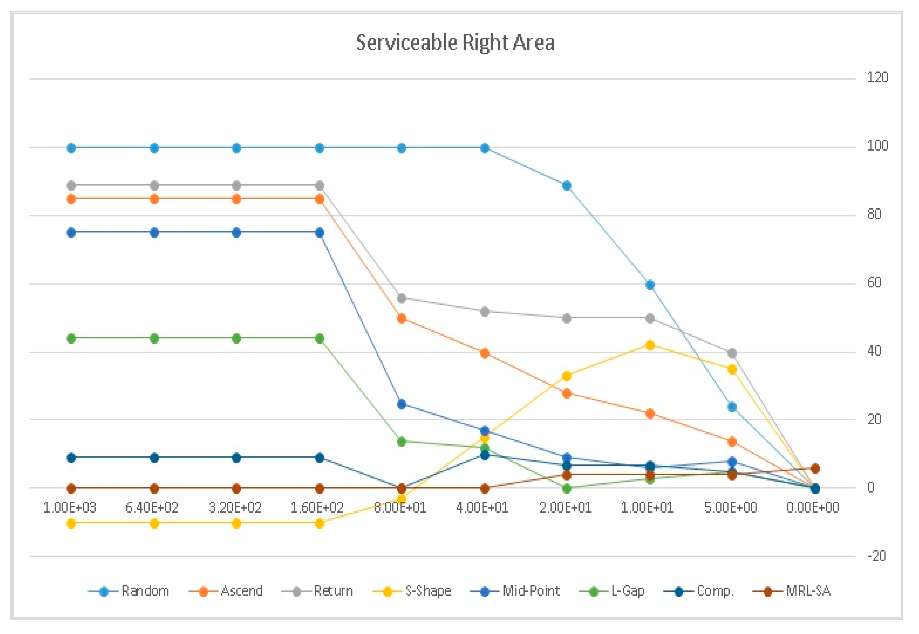
	Right area	4	I,J,K,L	350
3	Q1	3	A,E,I	500
	Q2	3	B,F,J	500
	Q3	3	C,G,K	500
	Q4	3	D,H,L	500

and illustrated in Figure 8, while the ANOVA results are illustrated in

Table 10. ANOVA for Q1, Q2, Q3 and Q4 comparison.

Source of Variation	SS	df	MS	F	p-Value	F Crit
Sample	200566.1	8	25070.77	247.6	8e−285	1.944
Columns	639676.2	6	106612.7	1053	0	2.105
Interaction	661237	48	13775.77	136.1	0	1.368
Within	184985.9	1827	101.2512
Total	1686470	1886

.

Computational results of the proposed model were solved by a solver with its default settings on a hp-core i3 Precision Workstation running under Windows 10. The I/O place selection in the left, right or middle will not be significant for the proposed heuristic, but S-Shape is preferable if it is in the right place and the composite method is preferable if it is in the middle, as illustrated in Figure 9, Figure 10 and Figure 11. Also, the layout is divided to Qi zones. The initial deviation of the request locations in Plan-A, and the modified locations in Plan-B are set to zero (i.e.,$I_0^S=I_0^R=0$). the location requested, updated and disposing are taken as $S^A=7$, $S^B=4, X^D=2$, respectively. $h^{PB}=4\le h^{PA}=5$ The locations backlogging is set to b ∈ {3, 4, 5, 6}, as shown in Table 8, to ensure all possible relations (i.e., less than, equal, or greater than) between$h^{PB}and b, h^{PA}and b$. The uncertain request has a mean ${\overline{d}}_t\in \left\{18,20,22\right\}$ and a standard deviation of $\sigma \in \left\{2,4\right\}$. In the proposed framework, the uncertain request $d_t$ can take any value from the interval ${\overline{[d}}_t-2\sigma ,{\overline{d}}_t+2\sigma ], i.e., {\widehat{d}}_t=2\sigma .$ Similarly; the uncertain updated requests have a mean ${\overline{r}}_t\in \left\{14,16,18\right\}$ and a standard deviation $\sigma \in \left\{2,4\right\}$. As a result, the uncertain updated locations $r_t$ can take any value from the interval ${\overline{[r}}_t-2\sigma ,{\overline{r}}_t+2\sigma ], i.e., {\widehat{r}}_t=2\sigma .$ Thus, combining all the parameter settings that have generated 72 instances for the average-case performance assessment, in total. While the costs of uncertainty ${\tau }_t^d$ are generated such that the probability of infeasibility at constraints (4) and (5) for t is less than 5%, the proposed costs of uncertainty ${\tau }_t^r$ are generated such that the probability of infeasibility at constraint (6) for t is less than 0.1%.

6. Conclusions

In this work, the Last Planner System used in the construction projects sector has evolved by a hybrid search algorithm that was used by combining MRL and SA through two sequential phases, and the sum of the route length value (e.g., illustrated in Figure 12) of the main route that results from MRL and backlogs-list of the unidirectional or bidirectional flow path to become the Lean Planner System. The performance of the proposed algorithm was tested using a wide set of data, and the results showed that the proposed MRL-SA algorithm was performing well, as illustrated in Figure 13. The main conclusions for the paper are summarized in the following points:

When the requests reach up to 60% of all locations that must be serviceable, the proposed heuristic MRL-SA presents the optimum route length, which has not proved costly when compared to the reviewed heuristic methods, but if the request size is considered, the Composite heuristic method is preferred to achieve the objective of the proposed Plan-A. Therefore, Table 6 illustrates the results of the analyses and a comparison between the proposed MRL-SA and the composite heuristic method. The published three policies (S-Shape, Largest Gap and Mid-point) have nearly the same performance. There are two cases affecting MRL-SA performance, first when the serviceable locations fall to less than 4.2%, while the second emerged when the requested locations for serviceable becomes more than 14% of the total requested using S-shape or MRL-SA, and these will be integrated together to achieve the objective.

The paper revealed that when the layout was divided into two halves (upper and lower) and the farthest points about the I/O position, the integration of the MRL-SA and Composite is preferred as illustrated in Figure 13 and can be deduced from Table 8. While, if the requested locations lay in the lower half, the integration between MRL-SA and the Return or Mid-point are preferred to execute Plan-A and Plan-B, as illustrated in Table 10.

When the requested serviceable locations are distributed vertically in three parallel regions, the Plan’s implementation of MRL-SA or another method will result in a short route, but with differences in cost, according to the requested distribution case.

7. Future Work

The same proposed algorithm that targets a reduction in the movement waste of Lean management, can be used for other applications. For example, improving the processes layout that has minimum backtrack direction and minimum transportation, whether in shop-floor or in inventory handling, which has been widely implemented as cited by Joël, R [26], but nowadays, this algorithm can be programmed to be a Mobile application to guide patients in hospitals to reduce their walks between examining rooms. This policy targets a reduction in the likelihood of patients meeting in aisles, which is especially relevant in the context of combat COVID19, as suggested by the WHO recommendations.

References

- Alshaimi, A.; Koskela, L. “Critical Evaluation if the Previous Delay Studies in Construction”. Proceedings of BuHu 8th International Postgraduate Research Conference, Prague, Czech Republic, 26–27 June 2008; Czech Technical University: Prague, Czech Republic, 2008. [Google Scholar]
- Azevedo, S.G.; Carvalho, H.; Duarte, S.; Cruz-Machado, V. Influence of Green and Lean upstream suplly chain management practices on business sustainability. IEEE Trans. Eng. Manag. 2012, 59, 753–765. [Google Scholar] [CrossRef]
- Remon, F.A.; Sherif, M.H. Applying lean thinking in construction and performance Improvement. Alex. Eng. J. 2013, 52, 679–695. [Google Scholar]
- Mohammad, H.E.; Islam, A.; Yasmine, A. A heuristics-based solution to the continuous berth allocation and crane assignment problem. Alex. Eng. J. 2013, 52, 671–677. [Google Scholar]
- Dassonville, L. Handbook for Implementing a Quality Management System in a National Mapping Agency. World Wide Web. Available online: http://www.eurographics.org/sites/default/files/handbook_V1.pdf (accessed on 10 January 2016).
- Laila, M.; Khodeir, R.O. Examining the interaction between lean and sustainability principles in the management process of AEC industry. Ain Shams Eng. J. 2018, 9, 1627–1634. [Google Scholar]
- Rodriguez, D.; Buyens, D.; Van Landeghem, H.; Lasio, V. Impact of lean production o n perceived job autonomy and job satisfaction: An experimental study. Hum. Factors Ergon. Manuf. Serv. Ind. 2016, 6, 159–176. [Google Scholar] [CrossRef]
- Cherrafi, A.; Elfezazi, S.; Chiarini, A. The integration of lean manufacturing, Six Sigma and sustainability: A literature review and future research directions for developing a specific model. J. Clean. Prod. 2016, 139, 828–846. [Google Scholar] [CrossRef]
- Brandstنtter, G.; Kahr, M.; Leitner, M. Determining optimal locations for charging stations of electric car-sharing systems under stochastic demand. Transp. Res. Part B 2017, 104, 17–35. [Google Scholar] [CrossRef]
- Jayawickrama, M.; Jayatilaka, P.R.; Kulatunga, A.K. Investigation of Level of Adaptation of Sustainability Concepts in Local Manufacturing Sector: A Case Study. In Proceedings of the 2nd Roundtable on SCP, Colombo, Sri Lanka, 21–22 February 2013. [Google Scholar]
- Ozcelik, F.A. Hybrid genetic algorithm for the single row layout problem. Int. J. Prod. Res. 2012, 50, 5872–5886. [Google Scholar] [CrossRef]
- Lenin, N.; Siva Kumar, M.; Islam, M.N.; Ravindran, D. Multi-objective optimization in single row layout design using a genetic algorithm. Int. J. Adv. Manuf. Technol. 2013, 67, 1777–1790. [Google Scholar] [CrossRef][Green Version]
- Chen, R.; Qian, X. Optimal charging facility location and capacity for electric vehicles considering route choice and charging time equilibrium. Comput. Oper. Res. 2020, 113, 104776. [Google Scholar] [CrossRef]
- Lenin, N.; Kumar, M.S.; Ravindran, D.; Islam, M.N.A. Tabu search for multi objective single row facility layout problem. J. Adv. Manuf. Syst. 2014, 13, 17–40. [Google Scholar] [CrossRef]
- Iliya, M. Waste collection inventory routing with non-stationary stochastic demands. Comput. Oper. Res. 2020, 113, 104798. [Google Scholar]
- Wang, W. Robotics and Computer Integrated Manufacturing. Robot. Comput. Integr. Manuf. 2020, 61, 101849. [Google Scholar] [CrossRef]
- Brevet, D. A dial-a-ride problem using private vehicles and alternative nodes. J. Veh. Routing Algorithms 2019, 2, 89–107. [Google Scholar] [CrossRef][Green Version]
- Benkebir, N. On a multi-trip vehicle routing problem with time windows integrating European and French driver regulations. J. Veh. Routing Algorithms 2019, 2, 55–74. [Google Scholar] [CrossRef]
- Gagarin, A.; Corcoran, P. 2018. Multiple domination models for placement of electric vehicle charging stations in road networks. Comput. Oper. Res. 2018, 96, 69–79. [Google Scholar] [CrossRef]
- Wu, F.; Sioshansi, R. A stochastic flow-capturing model to optimize the location of fast-charging stations with uncertain electric vehicle flows. Transp. Res. Part D 2017, 53, 354–376. [Google Scholar] [CrossRef]
- Blair, E.H. Regulation time Culture. Professional Regulation time. J. Prof. Saf. 2013, 58, 59–65. [Google Scholar]
- Shang, Y. Subgraph Robustness of Complex Networks Under Attacks. IEEE Trans. Syst. Man Cybern. Syst. 2019, 49, 821–832. [Google Scholar] [CrossRef]
- Tran, T.H.; Nagy, G.; Nguyen, T.B.T.; Wassan, N.A. An efficient heuristic algorithm for the alternative-fuel station location problem. Eur. J. Oper. Res. 2018, 269, 159–170. [Google Scholar] [CrossRef]
- Ahmed, M.A.; Adel, A.-E.I. Defect Control via Forecasting of Processes’ Deviation as JIDOKA Methodology. In Proceedings of the International Conference on Industrial Engineering and Operations Management, Bandung, Indonesia, 6–8 March 2018. [Google Scholar]
- Lu, C.C.; Yu, V.F. Data envelopment analysis for evaluating the efficiency of genetic algorithms on solving the vehicle routing problem with soft time windows. Comput. Ind. Eng. 2013, 63, 520–529. [Google Scholar] [CrossRef]
- Joël, R. Solving a real-life roll-on–roll-off waste collection problem with column generation. J. Veh. Routing Algorithms 2019, 2, 41–54. [Google Scholar] [CrossRef]