Dominance Conditions for Optimal Order-Lot Matching in the Make-To-Order Production System

Abstract

Order-lot matching is the process of assigning items in lots being processed in the make-to-order production system to meet the due dates of the orders. In this study, an order-lot matching problem (OLMP) is considered to minimize the total tardiness of orders with different due dates. In the OLMP considered in this study, we need to not only determine the allocation of items to lots in the production facility but also generate a lot release plan for the given time horizon. We show that the OLMP can be considered as a special type of machine scheduling problem with many similarities to the single machine total tardiness scheduling problem ($1||\sum T_i$). We suggest dominance conditions for the OLMP by modifying those for $1||\sum T_i$ and a dynamic programming (DP) model based on the dominance conditions. With two example problems, we show that the DP model can solve small-sized OLMPs optimally.

1. Introduction

Order-lot matching is the process of assigning items in work-in-progress (WIP) lots to orders in a make-to-order production system to meet the due dates of the orders. Typical examples for order-lot matching include the allocation of semiconductor chips in the semiconductor industry and the allotment of liquid crystal display (LCD) semi-products in the color-filter fabrication facility of thin film transistor liquid crystal display (TFT-LCD) industry. This study was motivated by a need of semiconductor company in Korea that produces memory chips and adopts make-to-order strategy. The order-lot matching problem is different from the lot sizing problem [1,2] in that lot sizes are not to be determined but fixed. Since order sizes are usually larger than lot sizes, an order is met with multiple lots. If all of the orders are met with the lots being processed at the production facility, the additional items must be released to the production facility. Therefore, in the manufacturing industries, which have a relatively long Turn-Around-Time (TAT), effective order-lot matching can improve the customer service level, such as the on-time-delivery rate and the levels of CPFR (Collaborative Planning, Forecasting, and Replenishment). Usually, order-lot matching is performed periodically in the make-to-order production system once every day or once every shift.

While a tremendous amount of research has been performed in the area of planning and scheduling, there is relatively little research on the order-lot matching problem (OLMP). The OLMP has mostly been studied to meet customers’ needs in the semiconductor manufacturing industry. The authors of [3,4,5,6,7,8] studied order-lot matching problems in the semiconductor assembly and/or test facilities. The authors of [9,10,11] studied order-lot matching problems in the wafer fabrication facility. [11] revealed the characteristics of the OLMP by suggesting the compact pegging method and showing that the OLMP is similar to an order sequence problem with the compact pegging method. Recently, [12] proposed priority rules for the OLMP by exploiting similarities between the OLMP and the single machine total tardiness scheduling problem $1||\sum T_i$.

Due to the computational complexity of the OLMP, previous literature employed a heuristic approach to solve the problem. In this study, however, we exploit characteristics of the OLMP and propose optimality conditions for the OLMP for the first time, which can be used for developing optimal solution algorithms. The rest of this paper is organized as follows. In the next section, problem description for the OLMP is given. Section 3 presents the dominance conditions, which establish precedence relations among the orders in optimal order sequences followed by a dynamic programming (DP) model based on the dominance conditions to solve the OLMP optimally. Two examples of the OLMP are solved using the dominance rules and the DP model in the following section. In the last section, a short summary and suggestions for further research are given.

2. Problem Description

The OLMP considered in this study is the same with the problem studied in [12], i.e., the problem of assigning items in lots currently being processed to orders with the objective of minimizing the total tardiness of the orders. Items can be assigned to any order if their product types are the same as that of the order. When the orders cannot be satisfied with lots in process, additional lots are to be released into the production system to satisfy all orders with the given production capacity.

Parameters	$N$	number of orders
	$L$	number of lots in process
	$T$	length of the planning time horizon (unit: day)
	i	index for order
	l	index for lot
	t	index for time period (unit: day)
	$q_i$	quantity of order i
	$Q_t$	limit on the total number of items that can be released at time t
	$d_i$	due date of order i (unit: hour)
	CT	(estimated) production cycle time from release to finish (unit: hour)
Variables	$w_l$	number of items included in lot l
	$r_l$	(estimated) remaining time of lot l (unit: hour)
	$C_i$	completion time of order i (unit: hour)
	${\tau }_i$	tardiness of order i (unit: hour)
	$x_{il}$	number of items in lot l assigned to order i
	$y_{it}$	number of items newly released lot into the production system at time t for order i
	$z_{il}$	equals 1 if lot l is used to satisfy order i, 0 otherwise
	$u_{it}$	equals 1 if there exist some lots newly released at time t to satisfy order i, 0 otherwise

The OLMP is formulated as a mixed integer linear program as below.

[OLMP] Minimize

$${\sum }_{i=1}^N{\tau }_i$$

(1)

subject to

$${\sum }_{l=1}^L{x}_{il}+{\sum }_{t=1}^T{y}_{it}=q_i \forall i$$

(2)

$${\sum }_{i=1}^N{x}_{il}\le w_l \forall l$$

(3)

$${\sum }_{i=1}^N{y}_{it}\le Q_t \forall t$$

(4)

$$x_{il}\le w_l{z}_{il} \forall i, l$$

(5)

$$y_{it}\le Q_t{u}_{it} \forall i, t$$

(6)

$$C_i\ge r_l{z}_{il} \forall i, l$$

(7)

$$C_i\ge \left(24t+CT\right)u_{it} \forall i, t$$

(8)

$${\tau }_i\ge C_i-d_i \forall i$$

(9)

$${\tau }_i\ge 0 \forall i$$

(10)

$$x_{il}\ge 0 \forall i, l$$

(11)

$$y_{it}\ge 0 \forall i, t$$

(12)

$$z_{il}\in \left\{0, 1\right\} \forall i, l$$

(13)

$$u_{it}\in \left\{0, 1\right\} \forall i, t$$

(14)

The objective of the problem is to minimize the total tardiness of all orders. Constraint (2) is for satisfying the order quantity with existing lots of items and/or newly released ones. Constraint (3) specifies the maximum possible number of items in a lot that can be assigned to orders. Constraint (4) represents a capacity of the production system, i.e., the maximum number of items that can be released at each period. Constraint (5) specifies the number of items in each lot assigned to different orders. Constraint (6) limits the total number of newly released items in each time period. Constraints (7) and (8) specify the completion time of each order. Note that $r_l$ in (7) is an estimated value, which can be calculated by the sum of processing time and waiting time. The waiting time varies dynamically according to the WIP level, so the estimated waiting time by the average of historical waiting time can be applicable. Constraint (9) represents the tardiness of each order. Equations (10)– (14) as constraints specify the ranges of the decision variables.

In [11], the authors proved the NP-hardness of the OLMP and the existence of an optimal order sequence for matching with lots. The order sequence represents processing priorities of orders; orders with higher priorities appear earlier in the sequence. They also proposed the order-lot assignment method called the compact pegging method for a given order sequence. In the compact pegging method, items (in lots) with less remaining time are assigned to orders with higher priorities, which results in the best lot-order assignment for the given order sequence. 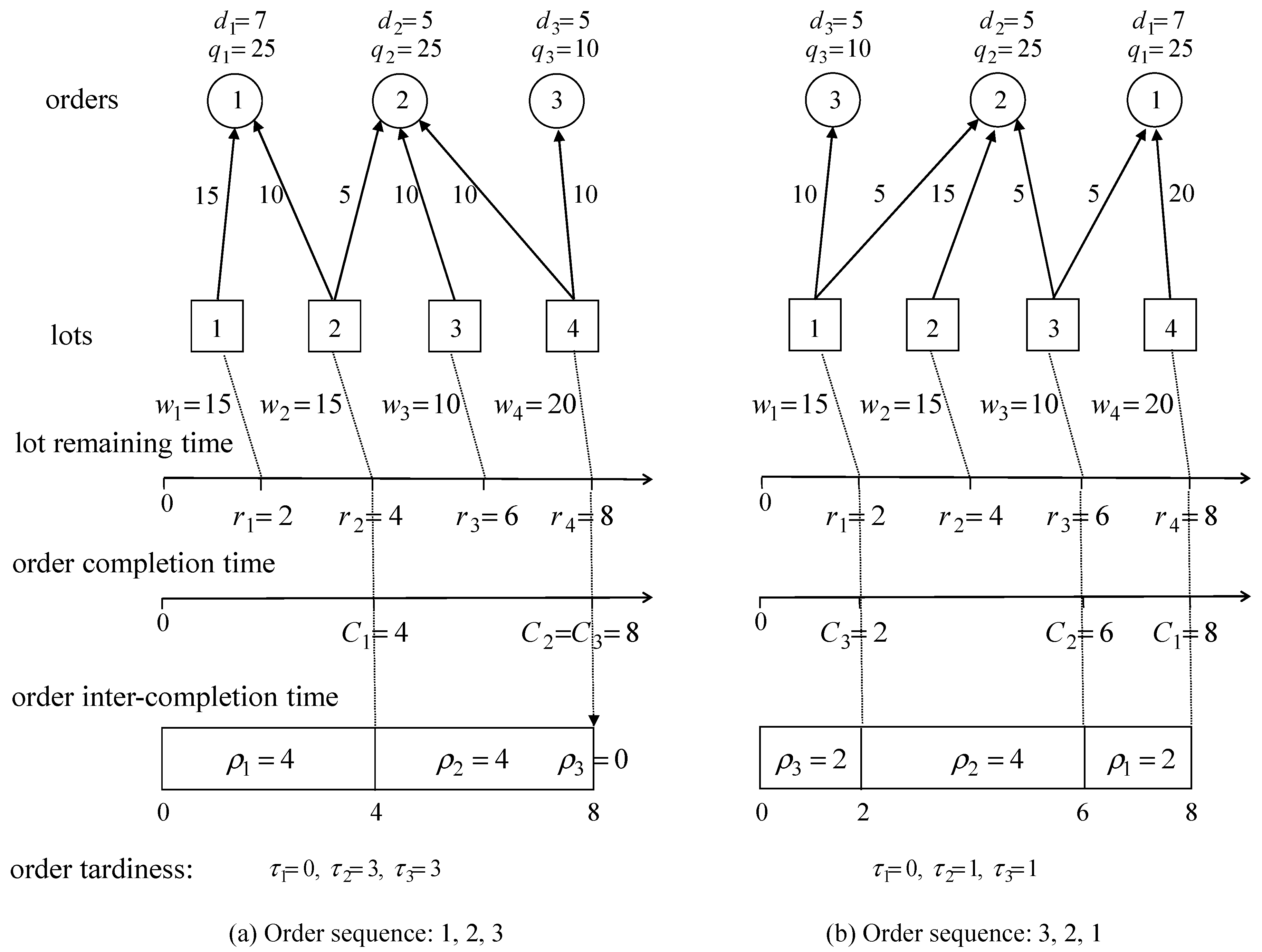Figure 1 illustrates how lots are assigned to orders using the compact pegging method for two order sequences. With the compact pegging method, the completion time of an order is equal to the largest remaining time of lots, which are assigned to the order and it is less than or equal to those of orders at later positions in the order sequence. As can be seen in the figure, orders with higher priorities have less completion times. Order completion times are subject to not only the order sequence but also order quantities, the number of lots, and the remaining times of lots, while job completion times in $1||\sum T_i$ are determined only by the job sequence. Let ${\rho }_i$ be the inter-completion time of order i, which is defined as the time duration between the completion times of order i and its precedent in the order sequence. The inter-completion time can be considered as the job processing time in $1||\sum T_i$. However, it is sequence dependent and can be equal to zero, unlike the job processing time: ${\rho }_1=4, {\rho }_2=4,{\rho }_3=0$ in Figure 1a and ${\rho }_1=2, {\rho }_2=4,{\rho }_3=2$ in Figure 1b although the sum of the inter-completion times is equal to the total completion time and it is a sequence-independent constant (${\sum }_{i=1}^3{\rho }_i=8$ in the example). Therefore, the OLMP cannot be converted into $1||\sum T_i$ but can be considered as a new type of machine scheduling problem with many similarities to $1||\sum T_i$.

Since the OLMP is an NP-hard problem, it is effective to develop efficient heuristic algorithms, such as [12], for solving large-sized problems. However, we can obtain optimal solutions for small and moderate-sized problems if there exist dominance conditions that can reduce the solution space significantly without affecting optimal solutions. In the following sections, we suggest dominance conditions for the OLMP and show how they can used to find the optimal solution.

3. Dominance Conditions

Since the OLMP has similar characteristics to $1||\sum T_i$, we exploit the dominance conditions of $1||\sum T_{i }$ to develop those of the OLMP. $1||\sum T_i$ is one of the most extensively studied problems in the literature, and, as a result, many theoretical theorems have been proposed to establish precedence relations among jobs in optimal job sequences. Among them, the most seminal ones are the Emmons’s dominance conditions [13] and the Lawler’s decomposition principle [14]. In this section, we show that the dominance conditions of Emmons [13] and Lawler [14] can be also applied to the OLMP. Since the dominance conditions for $1||\sum T_i$ cannot be directly applied to the OLMP due to the differences between the OLMP and $1||\sum T_i$ as mentioned before, we modified the dominance conditions of Emmons [13] and Lawler [14] for their application to the OLMP following the same manner of developing theories as Emmons [13] and Lawler [14].

At first, we propose theorems and derived corollaries that correspond to the Emmons’s dominance conditions [13]. Let $C(•)$ be the earliest possible total completion time for orders in order set $•$, i.e., the earliest possible time when all orders in order set $•$ can be completed. For example, $C\left(\left\{1\right\}\right)=4$, $C\left(\left\{2\right\}\right)=4$, $C\left(\left\{3\right\}\right)=2$, $C\left(\left\{1, 2\right\}\right)=8$, $C\left(\left\{1, 3\right\}\right)=6$, $C\left(\left\{2, 3\right\}\right)=6$, and $C\left(\left\{1, 2, 3\right\}\right)=8$ in Figure 1. Let B_i and A_i be the sets of orders that have been shown, at any point, to precede and follow order j in an optimal order sequence, respectively, and let $U_i^{\pi }$ be a set of orders that precedes order i in $\pi$.

Theorem 1.

For anytwo orders j and k with$q_j\le$, if $d_j\le \max (C\left(B_k\cup \left\{k\right\}\right), d_k)$, then order j precedes order k in at least one optimal order sequence (that is, $j\in B_k$and $k\in A_j$).

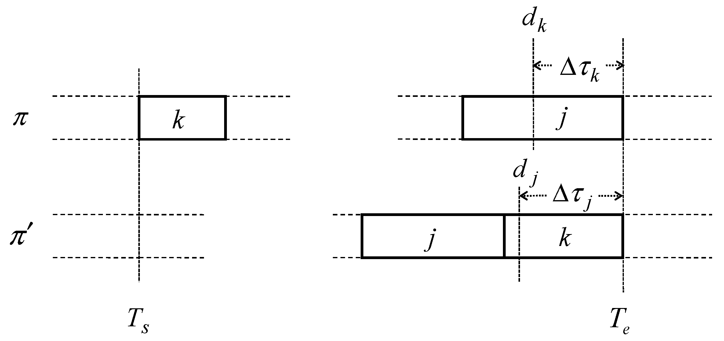
Proof. 

Consider order sequence $\pi \pi$ in which all orders in B_K precede order k, and order k precedes order j with $q_j\le q_k$. Let $T_s$ and $T_e$ be the times at which order k starts and order j ends, respectively (see Figure 2). Then, $T_s=C\left(U_k^{\pi }\right)$ and $T_e=C\left(U_j^{\pi }\cup \left\{j\right\}\right)$ . Additionally, let ${\rho }_k^{\pi }=C\left(U_k^{\pi }\cup \left\{k\right\}\right)-C\left(U_k^{\pi }\right)$ and ${\rho }_j^{\pi }=C\left(U_j^{\pi }\cup \left\{j\right\}\right)-C\left(U_j^{\pi }\right)$ be inter-completion times of orders k and j in order sequence $\pi$ , respectively. Let ${\pi }^{\prime }$ be an order sequence that is obtained by interchanging orders j and k in $\pi$ . Then, we have ${\rho }_j^{{\pi }^{\prime }}=C\left(U_k^{\pi }\cup \left\{j\right\}\right)-C\left(U_k^{\pi }\right)$ and ${\rho }_k^{{\pi }^{\prime }}=C\left(U_j^{\pi }\cup \left\{k\right\}\right)-C\left(U_j^{\pi }\right)$ . Since $q_j\le q_k$, ${\rho }_k^{\pi }\ge {\rho }_j^{{\pi }^{\prime }}$ and ${\rho }_j^{\pi }\le {\rho }_k^{{\pi }^{\prime }}$. Note there exists no (in) equality relationship between ${\rho }_j^{\pi }$ and ${\rho }_j^{{\pi }^{\prime }}$ (or ${\rho }_k^{\pi }$ and ${\rho }_k^{{\pi }^{\prime }}$ ) since they are sequence dependent. □

We show that interchanging the two orders does not increase the total tardiness. It is clear that all orders that precede order k or follow order j in the original sequence are unaffected when the two orders are interchanged. All orders between order k and j are completed earlier with their tardiness decreased or unchanged. We consider the following two cases to investigate the changes in tardiness of orders j and k after the interchange:

(a)

Suppose $d_j\le d_k$. We consider the following three subcases:

(a1)

If $d_j\le d_k<T_e$, as illustrated in Figure 2, then the decrease of tardiness of order j is $\Delta {\tau }_j=T_e-\max (T_s+{\rho }_j^{{\pi }^{\prime }}, d_j)$, the increase of tardiness of order k is $\Delta {\tau }_k=T_e-\max (T_s+{\rho }_k^{\pi }, d_k)$, and the net decrease due to the tow changes is $\Delta {\tau }_j-\Delta {\tau }_k=\max (T_s+{\rho }_k^{\pi }, d_k)-\max (T_s+{\rho }_j^{{\pi }^{\prime }}, d_j)$, which is nonnegative since $d_k\ge d_j$ and ${\rho }_k^{\pi }\ge {\rho }_j^{{\pi }^{\prime }}$.

(a2)

If $d_j\le T_e\le d_k$, $\Delta {\tau }_j-\Delta {\tau }_k=\Delta {\tau }_j\ge 0$.

(a3)

If $T_e<d_j\le d_k$, $\Delta {\tau }_j=\Delta {\tau }_k=0$. Thus, in all cases, the total decrease of tardiness is positive, or at worst zero, so the change should be made.

(b)

Suppose $d_j\le C\left(B_k\cup \left\{k\right\}\right)$, as also illustrated in Figure 2. Since $B_k\subseteq U_k^{\pi }$, $d_j\le C\left(U_k^{\pi }\cup \left\{k\right\}\right)$. Then, again, $\Delta {\tau }_j-\Delta {\tau }_k=\max (C\left(U_k^{\pi }\cup \left\{k\right\}\right), d_k)-\max (C\left(U_k^{\pi }\cup \left\{j\right\}\right), d_j)$ is nonnegative since $C\left(U_k^{\pi }\cup \left\{k\right\}\right)\ge \max (C\left(U_k^{\pi }\cup \left\{j\right\}\right), d_j)$.

According to Theorem 1, we can reduce the total tardiness by interchanging the positions of order j and k in the order sequence if order k precedes order j, $q_j\le q_k$, and $d_j\le \max (C\left(B_k\cup \left\{k\right\}\right), d_k)$. In Figure 1a, order 1 precedes order 3, $q_3\le q_1$ and $d_3\le d_1$, so we can reduce the total tardiness from six to two by interchanging order 1 and order 3 as shown in Figure 1b.

Corollary 1.1. 

If order j has the properties $q_j\le q_i$and$d_j\le \max (C\left(\left\{i\right\}\right), d_i)$for all$i\ne j$, then order j is the first in an optimal order sequence.

Proof. 

It is obvious by Theorem 1. □

Corollary 1.2.

If order j has properties $q_j\ge q_i$and$\max (C\left(\left\{j\right\}\right), d_j)\ge d_i$for all$i\ne j$, then order j is the last in an optimal order sequence.

Proof. 

It is obvious by Theorem 1. □

Corollary 1.3.

Let the least quantity sequence be an order sequence in which orders of fewer quantities are placed earlier in the sequence. Then, the least quantity sequence is optimal if it is identical with the earliest due date sequence.

Proof. 

It is straightforward by case (a) in the proof of Theorem 1. □

Theorem 2.

For any two orders j and k with$q_j\ge q_k$, if$d_k\ge \max (d_j, C\left({A^{\prime }}_j-\left\{k\right\}\right))$, where${A^{\prime }}_j=\left\{i; i\notin A_j\right\}$, then order j precedes order k (that is,$k\in A_j$and$j\in B_k$).

Proof. 

Consider sequence $\pi$ in which order k precedes order j, all orders in $B{}_j$ precede order j, and order j precedes all orders in $A{}_j$ . Let $T_s$ and $T_e$ be the times at which order k begins and order j ends, respectively. Since ${A^{\prime }}_j\supseteq U_j^{\pi }\cup \left\{j\right\}\supseteq U_k^{\pi }\cup \left\{k\right\}\cup \left\{j\right\}$, $C\left(U_j^{\pi }\cup \left\{j\right\}\right)\left(=T_e\right)\le C\left({A^{\prime }}_j\right)$ and $C\left(U_k^{\pi }\right)\left(=T_s\right)\le C\left({A^{\prime }}_j-\left\{j\right\}-\left\{k\right\}\right)$. Consider sequence ${\pi }^{\prime }$, which is obtained by moving order k to a position immediately after order j in $\pi$ (see Figure 3 ). Again, orders before $T_s$ and after $T_e$ are unaffected. Order j and all orders between orders k and j are now processed earlier, which can decrease their tardiness or leave it unchanged. Only order k can have an increase in tardiness (Equation (15)):

$$\Delta {\tau }_k=\{\begin{array}{c}{T}_e-C\left(U_k^{\pi }\cup \left\{k\right\}\right), \mathrm{if} d_k<C\left(U_k^{\pi }\cup \left\{k\right\}\right),\\ T_e-d_k, \mathrm{if} C\left(U_k^{\pi }\cup \left\{k\right\}\right)\le d_k<T_e,\\ 0, \mathrm{if} d_k\ge T_e.\end{array}$$

(15)

 □

Since $C\left(U_k^{\pi }\right)\le C\left({A^{\prime }}_j-\left\{j\right\}-\left\{k\right\}\right)$ and $d_k\ge C\left({A^{\prime }}_j-\left\{k\right\}\right))$, we have the following inequalities (Equation (16)):

$$C\left(U_k^{\pi }\cup \left\{k\right\}\right)\le C\left({A^{\prime }}_j-\left\{j\right\}\right)\le C\left({A^{\prime }}_j-\left\{k\right\}\right)\le d_k$$

(16)

Therefore, the alternative, $\Delta {\tau }_k=T_e-C\left(U_k^{\pi }\cup \left\{k\right\}\right)$, is ruled out. If $\Delta {\tau }_k=0$, then moving order k after order j does not increase the total tardiness. For $\Delta {\tau }_k=T_e-d_k>0$, since $d_k\ge d_j$, we have $d_j<T_e$. It follows that the decrease of tardiness of order j is $\Delta {\tau }_j=\left(T_e-d_j\right)-\max (C\left(U_k^{{\pi }^{\prime }}\right)- d_j, 0)=T_e-\max (C\left(U_k^{{\pi }^{\prime }}\right), d_j)=T_e-\max (C\left(U_j^{\pi }\cup \left\{j\right\}-\left\{k\right\}\right), d_j)$.

Thus, $\Delta {\tau }_j-\Delta {\tau }_k=d_k-\max (C\left(U_j^{\pi }\cup \left\{j\right\}-\left\{k\right\}\right), d_j)$. Since $d_k\ge \max (d_j, C\left({A^{\prime }}_j-\left\{k\right\}\right))$ and $C\left({A^{\prime }}_j\right)\ge C\left(U_j^{\pi }\cup \left\{j\right\}\right)$, $d_k\ge \max (C\left(U_j^{\pi }\cup \left\{j\right\}-\left\{k\right\}\right), d_j)$, i.e., $\Delta {\tau }_j\ge \Delta {\tau }_k$. Thus, postponing order k after order j is advantageous in this case.

Corollary 2.1.

If order j has properties$d_j\ge d_i$for all$i\ne j$and$d_j\ge C\left(\Omega -\left\{j\right\}\right)$, where $\Omega$is a set of all orders, then order j is the last in an optimal sequence.

Proof. 

If $q_j\ge q_i$, order i precede order j by Theorem 1. Otherwise, order i precedes order j by Theorem 2. □

Theorem 3.

For any two orders j and k with$q_j\le q_k$, if$d_k\ge C\left({A^{\prime }}_j\right)$, where${A^{\prime }}_j=\left\{i; i\notin A_j\right\}$, then order j precedes order k (that is,$j\in B_k$and$k\in A_j$).

Proof. 

Consider any sequence in which order j precedes all orders in $A_j$ and follows order k. We show that interchanging orders j and k can only decrease the total tardiness. Let $T_e$ be the time at which order j ends. Since $T_e\le C\left({A^{\prime }}_j\right)$ and $d_k\ge C\left({A^{\prime }}_j\right)$, $d_k\ge T_e$. This means that order k maintains zero tardiness after the interchange. Since all other orders are either remained unmoved or are advanced in time, the only possible change in tardiness is decreasing. □

Now, we propose properties and a theorem that correspond to the Lawler’s decomposition principle [14]. Let $C_j^{\pi }$ be the completion time of order j in order sequence $\pi$.

Property 1.

Let$\pi$be any order sequence which is optimal with respect to the given due dates$d_1, d_2,\dots , d_N$, and ${d^{\prime }}_j$be chosen such that

$$min(d_j, C_j^{\pi })\le {d^{\prime }}_j\le \max (d_j, C_j^{\pi })$$

(17)

Then, any sequence ${\pi }^{\prime }$ which is optimal with respect to the due dates ${d^{\prime }}_1, {d^{\prime }}_2,\dots , {d^{\prime }}_N$ is also optimal with respect to $d_1, d_2,\dots ,d_N$ (but not conversely).

Proof. 

This property came from Theorem 1 of Lawler [14] and can be directly applied to the OLMP when jobs are substituted as orders. Refer to the proof of Theorem 1 of Lawler [14].

Property 2.

There exists an optimal order sequence$\pi$in which all on time orders are in non-decreasing due date order.

Proof. 

Suppose order i follows order j in an optimal sequence $\pi$, where orders i and j under $d_i\le d_j$ are both on time in $\pi$. Then, moving order j after order i yields a sequence for which the total tardiness is no greater. □

Theorem 4.

Suppose that the orders are numbered in non-decreasing due date order, i.e.,$d_1\le d_2\le \dots \le d_N$(where $i<j$whenever$d_i=d_j$and$q_i\le q_j$). Let order k be such that$q_k={\max }_j(q_j)$. Then, there exists an optimal order sequence in which order k can be set in position $h\ge k$and the orders preceding and following order k are determined as$B_k=\left\{1, 2, \dots , k-1, k+1, \dots , h\right\}$and$A_k=\left\{h+1, \dots , n\right\}$.

Proof. 

Let $\pi$ be any order sequence that is optimal with respect to the given due dates $d_1, d_2,\dots , d_N$, and let ${\pi }^{\prime }$ be an order sequence which is optimal with respect to the due dates $d_1, d_2,\dots , d_{k-1}, {d^{\prime }}_k=\max (C_k^{\pi }, d_k), d_{k+1},\dots , d_N$. By Property 1, ${\pi }^{\prime }$ is also optimal with respect to the original due dates. It follows that $C_k^{{\pi }^{\prime }}=C_k^{\pi }$ and thus $C_k^{{\pi }^{\prime }}\le {d^{\prime }}_k$. By Theorem 1, any order j with $d_j\le {d^{\prime }}_k$ precedes order k in ${\pi }^{\prime }$. Any order j such that $d_j>{d^{\prime }}_k$ would be on time if it precedes order k in ${\pi }^{\prime }$, which means that such order follows order k in ${\pi }^{\prime }$ by Property 2. Thus, order k is preceded by all orders j such that $d_j\le {d^{\prime }}_k$ in ${\pi }^{\prime }$. Let h be chosen to be the largest integer such that $d_h\le {d^{\prime }}_k$, and the theorem is proved. □

Property 3.

Suppose that orders are numbered in non-decreasing due date order, i.e.,$d_1\le d_2\le \dots \le d_N$(where$i<j$whenever$d_i=d_j$and$q_i\le q_j$). Let order k be such that$q_k={\max }_j(q_j)$. Then, there exists at least one optimal order sequence in which order k is not placed in position h, where$k\le h\le N-1$and$C\left(\left\{i | 1\le i\le h\right\}\right)\ge d_{h+1}$.

Proof. 

By Theorem 4, there exists an optimal order sequence $\pi$ in which $B_k=\left\{1, 2, \dots , k-1, k+1, \dots , h\right\}$, where $k\le h\le N-1$. If $C\left(\left\{i | 1\le i\le h\right\}\right)\ge d_{h+1}$, set ${d^{\prime }}_k=C_k^{\pi }=C\left(B_k\cup \left\{k\right\}\right)=C\left(\left\{i | 1\le i\le h\right\}\right)$. Then, by Property 1, an optimal order sequence with respect to ${d^{\prime }}_k$ (say ${\pi }^{\prime }$) is also optimal with respect to $d_k$. By Theorem 4, order k is placed in position m in ${\pi }^{\prime }$ where $k\le m\le N-1$ and ${d^{\prime }}_k<d_{m+1}$. Since $d_{h+1}\le {d^{\prime }}_k=C\left(\left\{i | 1\le i\le h\right\}\right)<d_{m+1}$, $m>h$, which means that order k is not placed in position h in ${\pi }^{\prime }$. □

According to Theorem 4, the order set can be decomposed into two subsets by order k, i.e., $B_k$ and $A_k$. Thus, a DP model can be used to find the optimal order sequence, as was done in [14]. The following notation is used to define the DP model:

$$S\left(i, j, k\right)=\{l | i\le l\le j, q_l<q_k\}$$

$T\left(S\left(i, j, k\right), Q\right)$: the total tardiness for an optimal sequence of the orders in $S\left(i, j, k\right)$ when the most progressed Q items, i.e., Q items with the least remaining work, were already assigned to other orders and thus were not available any longer.

$C\left(S, Q\right)$: the total completion time for orders in S when the most progressed Q items were already assigned to other orders and thus they are not available any longer.

The DP model is given as:

$$\begin{gathered} T\left(S\left(i, j, k_{t-1}\right), Q\right)=\underset{0\le \delta \le j-k_t }{min}\{T\left(S\left(i, k_t+\delta , k_t\right), Q\right)+\max (0, C\left(\{l | i\le l\le \\ {k}_t+\delta \}\right), Q)-d_{k_t})+T\left(S\left(k_t+\delta +1, j, k_t\right), {\sum }_{i=1}^{k_t+\delta }{q}_i\right)\}, \mathrm{where} k_t=\underset{l}{argmax}\left\{q_l | l\in \\ S\left(i, j, k_{t-1}\right)\right\}. \end{gathered}$$

(18)

To select $k_t$ in Equation (18), ties are broken by choosing an order with the earliest due date. To apply the DP model, we set $i=1$, $j=N$, and $Q=0$ at first. The initial conditions for e Equation (15) are $k_0=0$, $q_0=\infty$, $T\left(\varnothing , Q\right)=0$, and $T\left(\left\{j\right\}, Q\right)=\max (0, C\left(\left\{j\right\}, Q\right)-d_j)$.

By Property 3, it is sufficient to consider only values of $\delta$ satisfying inequality $C\left(\left\{l | i\le l\le k_t+\delta \right\}\right)<d_{k_t+\delta +1}$. As a result, there may be a considerable reduction in the number of subproblems that must be solved. Let $\Psi =\{\delta | 0\le \delta \le j-k_t, C\left(\left\{l | i\le l\le k_t+\delta \right\}\right)<d_{k_t+\delta +1}\}$. (Here, it is assumed that $d_{N+1}=\infty$ for completeness of $\Psi$.) Then, Equation (18) can be rewritten as

$$\begin{gathered} T\left(S\left(i, j, k_{t-1}\right), Q\right)=\underset{\delta \in \Psi }{min}\{T\left(S\left(i, k_t+\delta , k_t\right), Q\right)+max(0, C\left(\{l | i\le l\le k_t+\delta \}\right), Q)- \\ {d}_{k_t})+T\left(S\left(k_t+\delta +1, j, k_t\right), {\sum }_{i=1}^{k_t+\delta }{q}_i\right)\}, \mathrm{where} k_t=\underset{l}{argmax}\{q_l | l\in S\left(i, j, k_{t-1}\right)\}. \end{gathered}$$

(19)

Since the development of Lawler’s decomposition theorem [14], there have been further theoretical developments in the decomposition theorem for $1||\sum T_i$ by many researchers, such as [15,16,17,18]. See [19] for a review on the latest theoretical developments on $1||\sum T_i$. The variants of Lawler’s decomposition theorem [14] could be also applied to the OLMP similarly.

4. Examples

We give two examples of the OLMP that can be solved optimally using the dominance rules and the DP model explained in Section 3.

<Example 1>

Table 1. Order data for Example 1.

i	1	2	3	4	5
$q_i$	10	40	20	15	50
$d_i$	10	10	15	25	30

and

Table 2. Lot data for Example 1.

L	1	2	3	4	5	6	7	8	9	10
$w_l$	10	10	20	20	10	15	20	20	20	20
$r_l$	5	5	10	20	20	25	30	35	40	50

show data for Example 1.

We apply the dominance rules corresponding to Emmons’s rule [13] to Example 1.

(a)

By Corollary 1.1, order 1 is the first since $q_1\le q{}_i$ and $d_1\le d{}_i$ for all $i>1$, which implies $B_2=\left\{1\right\}, B_3=\left\{1\right\}, B_4=\left\{1\right\}, B_5=\left\{1\right\}, \mathrm{and} A_1=\left\{2, 3, 4, 5\right\}$.

(b)

By Corollary 1.2, order 5 is the last since $q_5\ge q{}_i$ and $d_5\ge d{}_i$ for all $i<5$, which implies $A_1=\left\{5\right\}, A_2=\left\{5\right\}, A_3=\left\{5\right\}, A_4=\left\{5\right\}, \mathrm{and} B_5=\left\{1, 2, 3, 4\right\}$.

(c)

By Theorem 1, order 3 precedes order 2 since $q_3\le q{}_2$ and $d_3\le max(C\left(B_2\cup \left\{2\right\}\right)=20, d_2)$, which implies $B_2=\left\{1, 3\right\}$ and $A_3=\left\{2, 5\right\}$.

(d)

By Theorem 2, order 2 precedes order 4 since $q_4\le q{}_2$, $d_4>max(C\left({A^{\prime }}_2-\left\{4\right\}\right)=20, d_2)$. It follows that $B_4=\left\{1, 2, 3\right\}$ and $A_2=\left\{4, 5\right\}$. that $B_4=\left\{1, 2 3\right\}$ and $A_2=\left\{4, 5\right\}$.

According to (a)–(d), the optimal order sequence is 1, 3, 2, 4, 5 with the total tardiness of 20. Figure 4 illustrates the optimal order-lot matching for Example 1.

<Example 2>

Table 3. Order data for Example 2.

i	1	2	3	4
$q_i$	20	30	40	20
$d_i$	10	20	30	40

and

Table 4. Lot data for Example 2.

L	1	2	3	4	5	6	7
$w_l$	20	20	10	20	20	10	20
$r_l$	10	20	30	40	50	60	70

show data for Example 2. We apply the DP model based on the dominance rules corresponding to Lawler’s rules [14] to Example 2.

To apply the DP model, the initial conditions for Equation (16) are given as $i=1$, $j=N$, $t=1$, $Q=0$, $k_0=0$, $q_0=\infty$, and $d_5=\infty$.

We consider order set $S\left(1, 4, 0\right)=\left\{1, 2, 3, 4\right\}$. Since order 3 has the largest quantity among the considered orders, we obtain $k_1=3$. And since $\Psi =\{\delta | 0\le \delta \le 1, C\left(\left\{l | 1\le l\le 3+\delta \right\}\right)<d_{3+\delta +1}\}$, $C\left(\left\{1, 2, 3\right\}\right)=50>d_4$ and $C\left(\left\{1, 2, 3, 4\right\}\right)=70<d_5$, we obtain $\Psi =\left\{1\right\}$. Thus, Equation (16) yields:

$$\begin{gathered} T\left(S\left(1, 4, 0\right), 0\right)=T\left(S\left(1, 4, 3\right), 0\right)+\left[max(0, C\left(\left\{1, 2, 3, 4\right\}, 0\right)-d_3\right]+T\left(\varnothing , 110\right) \\ =T\left(S\left(1, 4, 3\right), 0\right)+40+0. \end{gathered}$$

Note that $S\left(1, 4, 3\right)=\left\{1, 2, 4\right\}$ and $C\left(\left\{1, 2, 3, 4\right\}, 0\right)=70$.

We set $t=2$ and consider order set $S\left(1, 4, 3\right)=\left\{1, 2, 4\right\}$. We obtain $k_2=2$ and $\Psi =\left\{0, 1\right\}$. Equation (16) yields:

$$T\left(S\left(1, 4, 3\right), 0\right)=\min \{\begin{array}{c}T\left(S\left(1, 2, 2\right), 0\right)+\left[max(0, C\left(\left\{1, 2\right\}, 0\right)-d_2\right]+T\left(S\left(4, 4, 2\right), 50\right)\\ T\left(S\left(1, 4, 2\right), 0\right)+\left[max(0, C\left(\left\{1, 4, 2\right\}, 0\right)-d_2\right]+T\left(\varnothing , 70\right)\end{array}$$

$$=\min \{\begin{array}{c}\left[max(0, C\left(\left\{1\right\}, 0\right)-d_1\left]+10+\right[max(0, C\left(\left\{4\right\}, 50\right)-d_4\right]=0+10+0=10\\ T\left(S\left(1, 4, 2\right), 0\right)+\left[max(0, C\left(\left\{1, 4, 2\right\}, 0\right)-d_2\right]+T\left(\varnothing , 70\right)=T\left(S\left(1, 4, 2\right), 0\right)+20+0.\end{array}$$

Note that $S\left(1, 2, 2\right)=\left\{1\right\}$, $S\left(4, 4, 2\right)=\left\{4\right\}$, $S\left(1, 4, 2\right)=\left\{1, 4\right\}$, $C\left(\left\{1, 2\right\}, 0\right)=30$, and $C\left(\left\{1, 4, 2\right\}, 0\right)=40$. Since $T\left(S\left(1, 4, 2\right), 0\right)\ge 0$, $T\left(S\left(1, 4, 3\right), 0\right)=10$. Thus, we obtain $T\left(S\left(1, 4, 0\right), 0\right)=50$ when an optimal order sequence is 1, 2, 4, 3. Figure 5 illustrates the optimal order-lot matching for Example 2.

5. Conclusions

In this study, we suggested dominance conditions for the OLMP by modifying those for $1||\sum T_i$ to establish precedence relations among the orders in optimal order sequences. These relationships can be used to curtail the solution space significantly. We suggested a DP model based on the dominance conditions to solve the OLMP optimally. The main contribution of this research is to propose the optimality conditions for the OLMP for the first time and show that the small-sized OLMPs can be solved optimally using the DP model. Further research is needed to improve the suggested dominance conditions and DP model to develop an optimal solution algorithm that can solve moderate-sized problem instances optimally within a reasonable time. Additionally, this study can be extended to various industries in which matching problems arise. For example, we can use the suggested model and approach to solve the cargo-ship matching problem [20] and the crane-ship matching problem [21] in the port industry.

References

1. Iris, C.; Yenisey, M. Multi-item simultaneous lot sizing and storage allocation with production and warehouse capacities. In Computational Logistics; Springer: Berlin/Heidelberg, Germany, 2012; pp. 129–141. [Google Scholar]
2. Phouratsamay, S.-L.; Kedad-Sidhoum, S.; Pascual, F. Two-level lot-sizing with inventory bounds. Discret. Optim. 2018, 30, 1–19. [Google Scholar] [CrossRef] [Green Version]
3. Knutson, K.; Kempf, K.; Fowler, J. Lot-to-order matching for a semiconductor assembly and test facility. IIE Trans. 1999, 31, 1103–1111. [Google Scholar] [CrossRef]
4. Fowler, J.; Knutson, K.; Carlyle, M. Comparison and evaluation of lot-to-order matching policies for a semiconductor assembly and test facility. Int. J. Prod. Res. 2000, 38, 1841–1853. [Google Scholar] [CrossRef]
5. Carlyle, M.; Knutson, K.; Fowler, J. Bin covering algorithms in the second stage of the lot to order matching problem. J. Oper. Res. Soc. 2001, 52, 1232–1243. [Google Scholar] [CrossRef]
6. Boushell, T.G.; Fowler, J.W.; Keha, A.; Montgomery, D.C. Evaluation of heuristics for a class-constrained lot-to-order matching problem in semiconductor manufacturing. Int. J. Prod. Res. 2008, 46, 3143–3166. [Google Scholar] [CrossRef]
7. Ng, T.S.; Sun, Y.; Fowler, J.W. Semiconductor lot allocation using robust optimization. Eur. J. Oper. Res. 2010, 205, 557–570. [Google Scholar] [CrossRef]
8. Sun, Y.; Fowler, J.W.; Shunk, D.L. Policies for allocating product lots to customer orders in semiconductor manufacturing supply chains. Prod. Plan. Control 2011, 22, 69–80. [Google Scholar] [CrossRef]
9. Wu, T.W. Modular demand and supply pegging mechanism for semiconductor foundry. In Proceedings of the 2003 IEEE International Symposium on Semiconductor Manufacturing, San Jose, CA, USA, 30 September–2 October 2003; pp. 325–328. [Google Scholar]
10. Bang, J.Y.; An, K.Y.; Kim, Y.D.; Lim, S.K. A due-date-based algorithm for order-lot matching in a semiconductor wafer fabrication facility. IEEE Trans. Semicond. Manuf. 2008, 21, 209–216. [Google Scholar]
11. Kim, J.G.; Lim, S.K. Order-lot pegging for minimizing total tardiness in wafer fabrication process. J. Oper. Res. Soc. 2012, 63, 1258–1270. [Google Scholar] [CrossRef]
12. Kim, J.G.; Lim, S.K.; Bang, J.Y. Lot-Order assignment applying priority rules for the single-machine total tardiness scheduling with nonnegative time-dependent processing times. Math. Probl. Eng. 2015, 2015, 434653. [Google Scholar] [CrossRef] [Green Version]
13. Emmons, H. One-machine sequencing to minimize certain functions of job tardiness. Oper. Res. 1969, 17, 701–715. [Google Scholar] [CrossRef]
14. Lawler, E.L. A “pseudopolynomial” algorithm for sequencing jobs to minimize total tardiness. Ann. Discret. Math. 1977, 1, 331–342. [Google Scholar]
15. Potts, C.N.; Van Wassenhove, L.N. A decomposition algorithm for the single machine total tardiness problem. Oper. Res. Lett. 1982, 1, 177–818. [Google Scholar] [CrossRef]
16. Szwarc, W. Single machine total tardiness problem revisited. In Creative and Innovative Approaches to the Science Management; Quorum Books: Westport, CT, USA, 1993; pp. 407–419. [Google Scholar]
17. Chang, S.; Lu, Q.; Tang, G.; Yu, W. On decomposition of the total tardiness problem. Oper. Res. Lett. 1995, 17, 221–229. [Google Scholar] [CrossRef]
18. Della Croce, F.; Tadei, R.; Baracco, P.; Grosso, A. A new decomposition approach for the single machine total tardiness scheduling problem. J. Oper. Res. Soc. 1998, 49, 1101–1106.
19. Koulamas, C. The single-machine total tardiness scheduling problem: Review and extensions. Eur. J. Oper. Res. 2010, 202, 1–7. [Google Scholar] [CrossRef]
20. Iris, Ç.; Christensen, J.; Pacino, D.; Røpke, S. Flexible ship loading problem with transfer vehicle assignment and scheduling. Transp. Res. Part B Methodol. 2018, 111, 113–134. [Google Scholar] [CrossRef] [Green Version]
21. Iris, Ç.; Pacino, D.; Røpke, S.; Larsen, A. Integrated berth allocation and quay crane assignment problem: Set partitioning models and computational results. Transp. Res. Part E Logist. Transp. Rev. 2015, 81, 75–97. [Google Scholar] [CrossRef] [Green Version]
Figure 1. Order-lot matchings using the compact pegging method.
Processes 08 00255 g001
Figure 2. The effect of interchanging two orders in an order sequence.
Processes 08 00255 g002
Figure 3. The effect of moving an order after another one in an order sequence
Processes 08 00255 g003
Figure 4. The optimal order-lot matching for Example 1
Processes 08 00255 g004
Figure 5. The optimal order-lot matching for Example 2.
Processes 08 00255 g005