Article

Computational Study in Bottom Gas Injection Using the Conservative Level Set Method

by
Jorge E. Rivera-Salinas
1,*,
Karla M. Gregorio-Jáuregui
2,
Alejandro Cruz-Ramírez
2,
Víctor H. Gutierréz-Pérez
3,
José A. Romero-Serrano
2,
Seydy L. Olvera-Vazquez
3,
Heidi A. Fonseca-Florido
4 and
Carlos A. Ávila-Orta
5
1
Catedrático CONACyT—Departamento de Procesos de transformación, Centro de Investigación en Química Aplicada—CIQA, Saltillo 25294, Coahuila, Mexico
2
Departamento de Ingeniería en Metalurgia y Materiales, Instituto Politécnico Nacional, Escuela Superior de Ingeniería Química e Industrias Extractivas—ESIQIE, UPALM, México City 07738, Mexico
3
Departamento de Formación Profesional Específica, Instituto Politécnico Nacional—Unidad Profesional Interdisciplinaria de Ingeniería campus Zacatecas—UPIIZ, Zacatecas 98160, Mexico
4
Catedrático CONACyT—Departamento de Materiales Avanzados, Centro de Investigación en Química Aplicada—CIQA, Saltillo 25294, Coahuila, Mexico
5
Departamento de Materiales Avanzados, Centro de Investigación en Química Aplicada—CIQA, Saltillo 25294, Coahuila, Mexico
*
Author to whom correspondence should be addressed.
Processes 2020, 8(12), 1643; https://doi.org/10.3390/pr8121643
Submission received: 13 November 2020 / Revised: 9 December 2020 / Accepted: 9 December 2020 / Published: 12 December 2020
(This article belongs to the Special Issue Applied Computational Fluid Dynamics (CFD))

Abstract

:
This paper presents a computational study on bottom gas injection in a cylindrical tank. The bubble formation at submerged orifices, bubble rising, and interactions between bubbles and bubbles with the free surface were studied using the conservative level set method (CLSM). Since the gas injection is an important technique in various fields and this process is quite complicated, the scenario was chosen to quantify the efficacy of the CLSM to describe the gas-liquid complex interactions with fast changes in the surface tension force and buoyancy force. The simulation accuracy is verified with the grid convergence index (GCI) approach and Richardson Extrapolation (RE) and is validated by comparing the numerical results with experimental observations, theoretical equations, and published data. The results show that the CLSM accurately reproduces the bubble formation frequency, and that it can handle complicated bubble shapes. Moreover, it captures the challenging phenomena of interaction between bubbles and free surface, the jet of liquid produced when bubbles break through the free surface, and the rupture of the film of liquid. Therefore, the CLSM is a robust numerical technique to describe gas-liquid complex interactions, and it is suited to simulate the gas injection operation.

1. Introduction

Gas-liquid reactors are used in a wide variety of applications in the chemical, petrochemical and metallurgy industries, etc. Because of its effectiveness, the gas injection processes have been widely investigated experimentally and numerically to understand the flow patterns of these systems.
Experimental studies are good options to understand the underlying mechanism in bubble dynamics. In certain regimes, interference appears in the measuring of characteristics relative to the flow, for instance, the pressure distribution and velocity field around the bubbles due to the rapid deformation that the bubble shape can undergo during its rise through the liquid. This problem poses limits for the scope of the experimental studies to the regime where only small bubble deformations exist, and the bubble shape is relatively stable [1].
Analytic studies and empirical correlations are normally formulated to study the global characteristics of the process, such as the average bubble size, volume fraction, the frequency of bubble formation, etc.
Although experimental studies can observe a series of new phenomena [2], they can take more time and have higher expenses than numerical studies [3]. As a result, in the significant progress in modeling of two-phase flow and the increasing power of computational resources, the numerical simulation offers scope to study the complex phenomena in bubble dynamics for a wide range of conditions. Moreover, it has been shown that the computational fluid dynamics (CFD) modelling of two-phase flow could exhibit better accuracy than the empirical correlations in the predictions of global characteristics [4]. Therefore, numerical studies have been widely used to extend the range of research into bubble formation, even beyond experimental studies [5]. Consequently, the two-phase flow simulation and experimental studies complement each other efficiently to achieve a deep insight into the flow patterns and have made significant advances in recent decades.
At this time, there is a wide variety of models coupled to the Navier-Stokes equations for simulating two-phase flow and free surface problems. In two-phase flow it is well known that energy, mass and momentum transfer rates are quite sensitive to the flow patterns, hence the progress in understanding a wide range of phenomena in two-phase flow, such as in the case of the bottom gas injection process, requiring accurate information about the flow structure.
Two-phase flow predictions with contact lines may dramatically vary for the same system, depending on the modelling parameters; e.g., discretization, mesh density, boundary conditions and technical parameters of the method to track the interface such as the level of reinitialization, among others. Incorrect selection of parameters may yield a smooth solution without physical meaning, leading to misleading conclusions. Therefore, when using a method to track the interface of the fluids, there are many pitfalls may render the results invalid [6]. In this context, validation and verification are fundamental concepts that determine the accuracy of the model and the numerical uncertainty of the solution, respectively. Moreover, complicated methods to track the interface means that much effort is needed to reproduce a result, therefore simple methods are preferable.
A popular technique in front capturing is the volume of fluid (VOF) method [7,8] because it ensures discrete mass conservation when accurate advection algorithms are used even for a relatively coarse mesh. Some approaches for the discrete solution of the VOF equation are the geometrical advection and a pseudo-Lagrangian technique. However, the drawbacks of the VOF method is that the local curvature computation of the interface is not satisfactory at all in some applications because of the discontinuity of the color function at the interface [9], which puts constraints on the geometric advection algorithm to accurately evolve the VOF scalar. Therefore, when an explicit treatment of the surface tension is employed, the contact angle condition and the stringent stability constraint on the time step must be imposed accurately.
The standard level set (LS) method [10,11] is an efficient method to compute the local curvature more accurately than the VOF method because in the LS method the function ϕ varies smoothly across the interface. With the LS method, the merging or break-up of the interface can be handled automatically without specific algorithms. However, a severe drawback to this method is that it is prone to a lose/gain mass of the fluid in a nonphysical manner. The technique called coupled level set volume of fluid (CLSVOF) method [12,13] combines the advantages of both the LS and the VOF. With this coupling, mass conservation from the VOF function and accurate computation of the curvature from the level set function are achieved. Although this method combines the complementary advantages of both the LS and the VOF method, it is more complicated because both the VOF and LS functions need to be solved and coupled. Moreover, as the modelling parameters increase, the pitfall arises while using complex methods.
Due to the simplicity and the ability of the standard LS method to accurately model two-phase flows, different techniques to overcome the mass conservation issue with the LS method were proposed by Sussman et al. [14], Herrmann [15,16], Olsson and Kreiss [17] and Wang et al. [18] Among the different attempts to alleviate the mass conservation issue, the simplicity of the original method is retained in the conservative level set method (CLSM) of Olsson and Kreiss [17]. In this signed distance function, ϕ of the standard method [10,11] is replaced with a hyperbolic tangent profile, and the interface contour is represented by using a Heaviside function bounded to interval [0, 1] where the interface is defined on ϕ = 0.5 , rather than the level set function. In a later work by Olsson et al. [19], they improved the CLSM by the modification of the reinitialization step, besides a finite element discretization and an adaptive mesh control procedure that were also presented in that work. For the improvement of the LS method, a reinitialization procedure was formulated as a conservation law so that together with the regularized characteristic function (the Heaviside function as a piecewise constant function), oscillations are damped. Using the regularized function and its preserving of the smooth profile in the reinitialization procedure, the spurious currents and the oscillations in the pressure are not introduced as the interface is advected. The solution of the mass conservation issue of the LS method allows the model to be used successfully in applications such as bubble formation [20], bubble rise [17,18,21] and bubble bursting at the free surface [14], among many others. It is important to remark that new formulations of the conservative level set method has been presented using different reinitialization procedures to improve the robustness of the CLSM [22,23].
There are published studies on some stages that occur in the gas injection process, such as the bubble formation, bubble rise and bubble bursting using an interface capturing method to track the interface. However, few studies that simulate the full process of bottom gas injection using front capturing methods are available in the literature. The Level Set formulated by Sussman et al. [14] has been used to study at the same time the stages involved in the bottom gas injection [24]. This study is focused on the rising behavior of gas bubbles and the bubble formation process from an orifice embedded to simulate the effects of solid concentrations on bubble formation and raise behavior. Valencia et al. [25] simulated the full process of bottom gas injection using the VOF method implemented in the Fluent software. In this work, simulations to explore numerically the growth, rise and the interaction with the upper air-water interface of bubbles generated by injection with a submerged orifice, were used. Comparison against theoretical predictions showed non-negligible differences attributed to the effect of wall adhesion.
The requirements for design and optimization of the gas injection operations need accurate quantitative information about such flow. These phenomena depend strongly on the flow structure. Two phase-flow simulations are essential for the calculation of production rates to design a more efficient process, so the studies to verify the capability of the currently available numerical methods to describe interfacial motions are very useful. Especially considering that the key issue to achieve a comprehensive analysis of the problem is the tracking of the interfaces. To this date, owing to the complexity of two-phase flow, their simulations remain a great challenge [26]. Based on the broad front capturing methods available to simulate two-phase flow, comparative testing studies have been carried out to identify the methods that are best suited for an accurate description and better predictions in modeling a particular problem. In [20], the growth and detachment of an isolated air bubble injected through a single orifice in the axiymmetric domain were considered using the VOF method, the LS method and the coupled VOF with LS (CLSVOF). It was found that the LS method consistently predicted the bubble detachment volume and time, with errors lower than 2%, while the VOF method produces the least accurate results with earlier bubble detachment and smaller volumes, whereas the CLSVOF method modeled significant bubble oscillations, which were not observed experimentally. Carlson et al. [27] tested the accuracy of both the VOF method and the LS method for the study of slug flow. The VOF method did not correctly predict the slug flow pattern under the conditions studied. The accuracy of the diffuse interface or phase-field approach and the CLSM to capture the coalescence process of two ferrodroplets, was investigated in [28]. Comparison against analytical solutions showed that the phase-field approach results are more accurate than the results of CLSM when the magnetic effect dominates over the surface tension effect; that is to say, when there are large topological deformations produced by large uniform magnetic fields. More comparative testing studies and the feasibility to simulate a specific application can be found elsewhere [29,30].
In this work, the effectiveness of the CLSM to simulate the bottom gas injection process is tested. The aim is to examine the efficacy and accuracy of this (relatively simple) approach to capture complicated gas-liquid interface motions with challenging phenomena with fast changes in the surface tension force (associated to curvature changes) and buoyancy force [31], such as those arising naturally in the gas injection process. Phenomena such as bubble formation from an orifice, the bubble rising close to the free surface and the bubble bursting into small droplets are covered. Therefore, this paper contributes to the documentation of applicability of the CLSM in complex two-phase multi-scale problems satisfyingly simulated.
For the conditions of the problem, the air is blown through an orifice placed at the center of the bottom of a recipient containing water. The problem also takes into account the deformation of the free surface gas-liquid caused by the impingement of the bubbles, which produce a jet of liquid when they break. For validation, the results were compared against numerical data computed with the VOF (using a Piecewise Linear Interface Calculation approach) method reported in the literature [25]. Moreover, qualitative comparisons of the computational results for the free surface behavior against experimental observations were made to further validate the numerical model. The simulation accuracy is verified with the grid convergence index (GCI) approach and Richardson Extrapolation (RE).

2. Basic Equations and Numerical Scheme

The equations governing the motion of an unsteady, immiscible and incompressible two-phase flow are essentially the Navier-Stokes equations. In gas-liquid two-phase flow, the main body forces which govern are the surface tension force ( F s t ) and the acceleration due to gravity ( g ). The buoyancy effect arises from the source term ( ρ g ). The equations can be written as
ρ ( ϕ ) u t + ρ ( ϕ ) u u = p + [ μ ( ϕ ) ( u + u T ) ] + ρ ( ϕ ) g + F s t
Together with the divergence-free condition.
u = 0
where u denotes the velocity field and p the pressure field. ρ ( ϕ ) and μ ( ϕ ) are the discontinuous density and viscosity fields, respectively. The density and viscosity are defined in terms of the level set function ϕ to smooth the jump conditions in the properties of the materials across the interface. The function ϕ is defined in the domains of the mixture of fluids and it is a Heaviside function that distinguishes the two phases varying smoothly from 0 to 1 across the interface.
ϕ ( x , y , t ) { < 0.5   if   ( x , y )     gas   domain   = 0.5   if   ( x , y )     interface > 0.5   if   ( x , y )     water   domain
ρ ( ϕ ) = ρ g + ( ρ l ρ g ) ϕ
μ ( ϕ ) = μ g + ( μ l μ g ) ϕ
The system is assumed to be isothermal. The gas density varies according to the ideal gas law, since the density of the liquid phase is three orders of magnitude higher than that of the gas phase. The surface tension is recast into a volume force in the Navier-Stokes equation and is formulated as the divergence of the capillary pressure tensor [32]:
F s t = T
T = σ ( I ( n n T ) ) δ
Here I is the identity matrix. The δ -function is approximated by a smooth Dirac delta function centered at the 0.5 isocontour of ϕ according to
δ = 6 | ϕ ( 1 ϕ ) | | ϕ |
The geometrical parameters as the curvature κ and the normal n to the interface are calculated along the 0.5 isocontour of the level set variable as follows
κ = n | ϕ = 0.5
n = ϕ | ϕ | | ϕ = 0.5
The equation governing the transport of the ϕ function is a hyperbolic partial differential equation, where the interface is advected by the local velocity field u . However, this convection equation is not very stable. Thus, to improve stability, a small amount of viscosity is added to avoid a discontinuity at the interfaces as well as an artificial compression flux in the normal direction [16] ( ϕ ( 1 ϕ ) n ). All of this is to maintain the resolution of sharp changes in properties at the interface. The equation governing the convection and the reinitialization of ϕ is given as
ϕ t + u ϕ = γ ( ε ϕ ϕ ( 1 ϕ ) ϕ | ϕ | )
The terms on the left-hand side represent the correct advection of the interface, while the terms on the right-hand side are necessary for the numerical stability control. The parameter ε represents the thickness of the transition layer, and it is desirable to keep ε as small as possible to give better conservation of the area bounded by the 0.5 contour of ϕ . On the other hand, since the method is coupled with the incompressible Navier-Stokes equations, a small value of ε will reduce the smearing of density, viscosity and surface tension [19]. A recommended value is half the coarsest mesh size (in this work, the coarsest mesh size in the simulations was 0.4 mm). The parameter γ determines the amount of reinitialization of the level set function and it helps to preserve the interface thickness constant. γ is assumed to be an artificial diffusion parameter. In this step, the Equation (11) reaches a steady state by pure diffusion without any convection. A too-small value of γ causes the interface to not maintain a constant value and oscillations can appear because of numerical instabilities. On the other hand, an excessively large value causes the interface to move incorrectly. A suitable value for γ is the maximum magnitude of the velocity field u [33]. During the bubble formation stage, the maximum superficial velocity of the gas varies significantly because of the neck radius reduction. Therefore, the reinitialization parameter that is good at the time when the neck of the bubble is formed would be very high after the pinch-off stage. If γ is represented by a piecewise function during the entire period of operation, the free surface moves nonphysically (jaggy interface) at the beginning, because it remains essentially quiescent until the first bubble impingement at the upper gas-liquid surface. Thus, after some ad hoc intervention, the choice of the γ was set to a constant value of 1 m/s. With this value the interface dynamics of the overall process are not sensitive to γ .
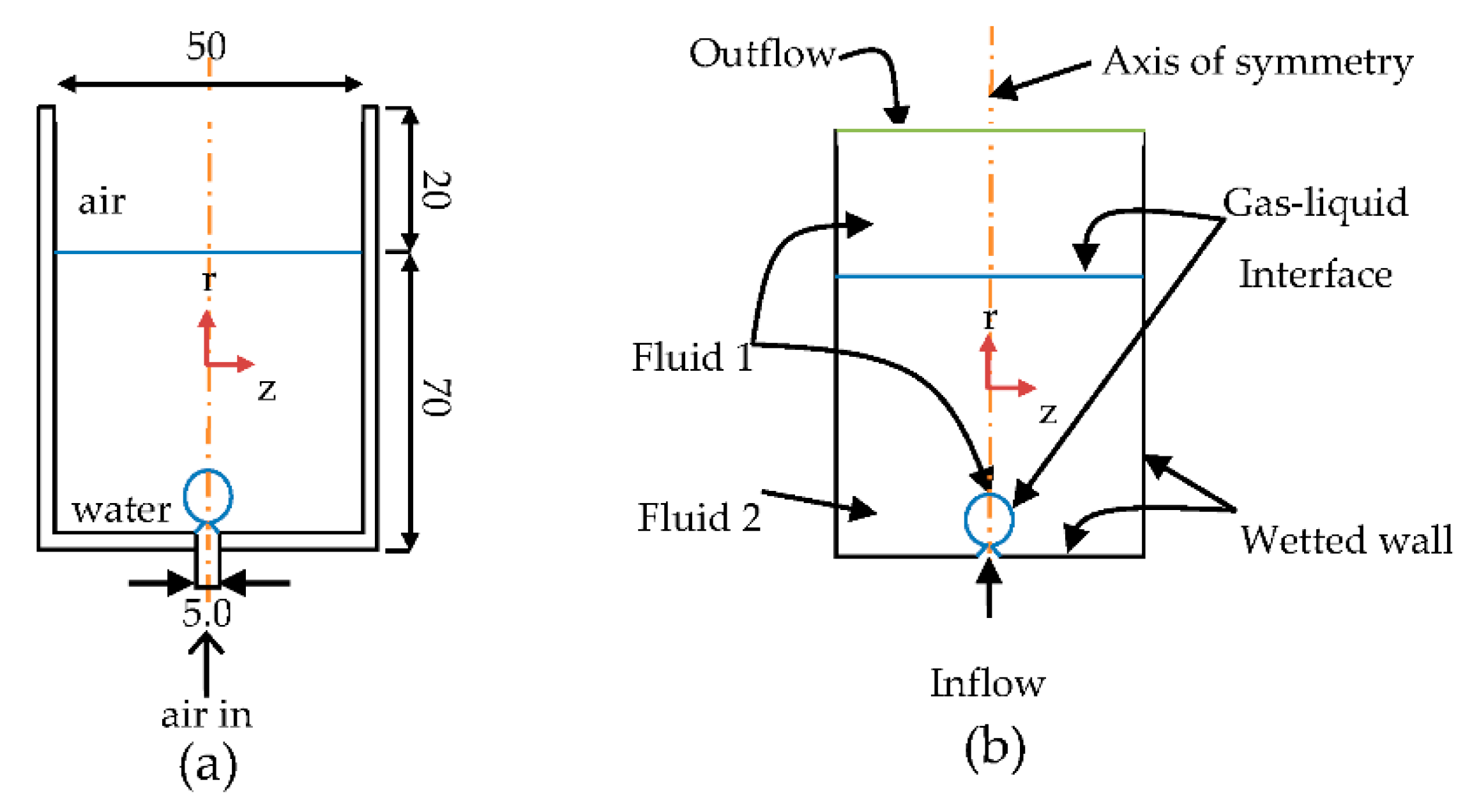
Figure 1 shows the solution domain used for the numerical computations of the bottom air injection into quiescent water. The physical dimensions are in millimeters and the boundary conditions used in this work are also shown. The diameter of the bottom orifice is 2.5 mm, and air flows through the orifice to a constant velocity of 0.2 m/s assuming a fully developed laminar flow where the average velocity profile is parabolic. It is assumed that the vessel to be made of a polymer and the contact angle between the liquid and solid walls is 110°. The parameters employed to perform the simulation were based on the conditions numerically studied in [25] using the VOF method. The gas is let go from the solution domain at the upper part of the vessel where outflow pressure was set to 1 Pa.
Due to the symmetry of the system about the vertical axis, a two-dimensional axisymmetric problem was used to solve in time-dependent and spatially the governing equations of fluid flow and interface capturing. Effects of azimuthal instabilities are ignored and may be important. This model was developed using the CFD module of COMSOL Multiphysics, where equations are solved using the Galerkin finite element method. The momentum and continuity equations were coupled in terms of the primitive variables u and p. The use of Galerkin formulation in problems which involve advection terms that dominate over diffusive terms tend to produce numerical instabilities. These result in spurious node to node oscillations in the velocity field, so the inclusion of the Streamline Upwind/Petrov-Galerkin method was used to stabilize the Navier-Stokes equations and the level set equations. The stabilization is achieved by adding a term to the Galerkin formulation for both incompressible and compressible flow by modifying the standard Galerkin weighting functions. This additional term prevents the oscillations caused by the presence of the advection term by adding a streamline upwind perturbation, which acts only in the flow direction [34].
The level set equation requires initialization at time t = 0 and u = 0 to define the initial position of the interface and to ensure the smooth initial solution of the level set variable, and then this initial solution is used to start the time-dependent simulations. The numerical algorithm employs the same methodology as presented in [19], with the main difference that they used the projection method to overcome the incompressibility constraint in the Navier-Stokes equations. The projection method is well suited for low Reynolds number calculations. It allows resolving the equations for the velocity and pressure in a segregated manner at each time step, reducing the amount of memory needed in the computing. The CFD solver of COMSOL Multiphysics (5.2a, COMSOL Inc. Burlington, MA, USA, 2016) is for general problems, which can include complicated boundary conditions. It uses by default a fully coupled solution strategy for the primitive variables ( u , p) using mixed methods. In mixed methods, the interpolation functions for pressure and velocity are chosen one order lower for pressure than those for the velocity to avoid pressure oscillations in the pressure field (due to the Babuska-Brezzi (B-B) inf-sup condition [35]). However, the software also allows for the use of combinations of an equal or higher order of interpolation functions for the velocity components and pressure field. Moreover, it also includes the incremental pressure correction scheme version of the projection method to solve in a segregated manner. In this work, the interpolation functions to represent the velocity and pressure were of the type P2-P1 even though the Petrov-Galerkin formulation of the problem circumvents the B-B inf-sup condition and piecewise quadratic P2 finite elements for the level set function.

2.1. Temporal Discretization

The temporal terms in the Navier-Stokes equations and level set equation were discretized in an implicit fashion by using a second-order backward difference formula (BDF) technique. The time steps are controlled by the numerical solver (adaptive time-stepping), but the numerical accuracy was checked by doing a convergence study where further mesh refinement and the decrease in the values of the relative tolerance (to lower the adaptive time step size in the solver) do not produce visible changes in the results (to ensure mesh independent, a mesh with a total of 1.7 × 10 5 elements has been retained). As mentioned above, in this work the adaptive time stepping option was used (BFD) since this implicit method is stable and has an efficient time step control. Thus, the appropriated Courant Friedrich Lewy (CFL) number was determined by the solver. Then, the time steps are updated as needed to achieve numerical stability, and according to the accuracy of the solution while it meets the specified relative tolerance ( 1 × 10 5 ). From the convergence plot reported by the solver (not shown here), it was observed that the smallest time step in the computation was Δ t = 4 . 5   × 10 5 , while the bigger time step was about Δ t = 9 . 2   × 10 4 . To accelerate the convergence rate, scaling factors for the variables u and p were set to 1 and 1000, respectively. With these values in the scaling variables, the convergence was accelerated. Convergence within each time step was tracked in the solver log where no failures were reported. Fixed meshes with unstructured triangular elements were used. The system of nonlinear equations was solved using the damped Newton method with a constant value equal to one for the damping factor. With such values for the damping factor, the nonlinear solver was stable and convergences were reasonably fast. The linear system of equations that arises at each Newton iteration was solved by a direct solver such as PARDISO. The full solution shown in the figures of the results section was obtained by mirroring in the symmetry plane.

2.2. Mesh Resolution

Simulations were run over three fixed meshes: coarse ( N 3 = 5900 elements), intermediate ( N 2 = 21,196 elements) and fine ( N 1 = 175,202 elements). A convergence study of mesh refinement was performed to quantify the discretization error of the solutions. Uncertainty estimates were calculated with the Grid Convergence Index (GCI) and performed with a Richardson extrapolation (RE). Detailed information for the performing of the later methods GCI and RE can be found at ASME V and V 20-2009 (this standard address verification and validation (V and V) in CFD and HT) [36] and [
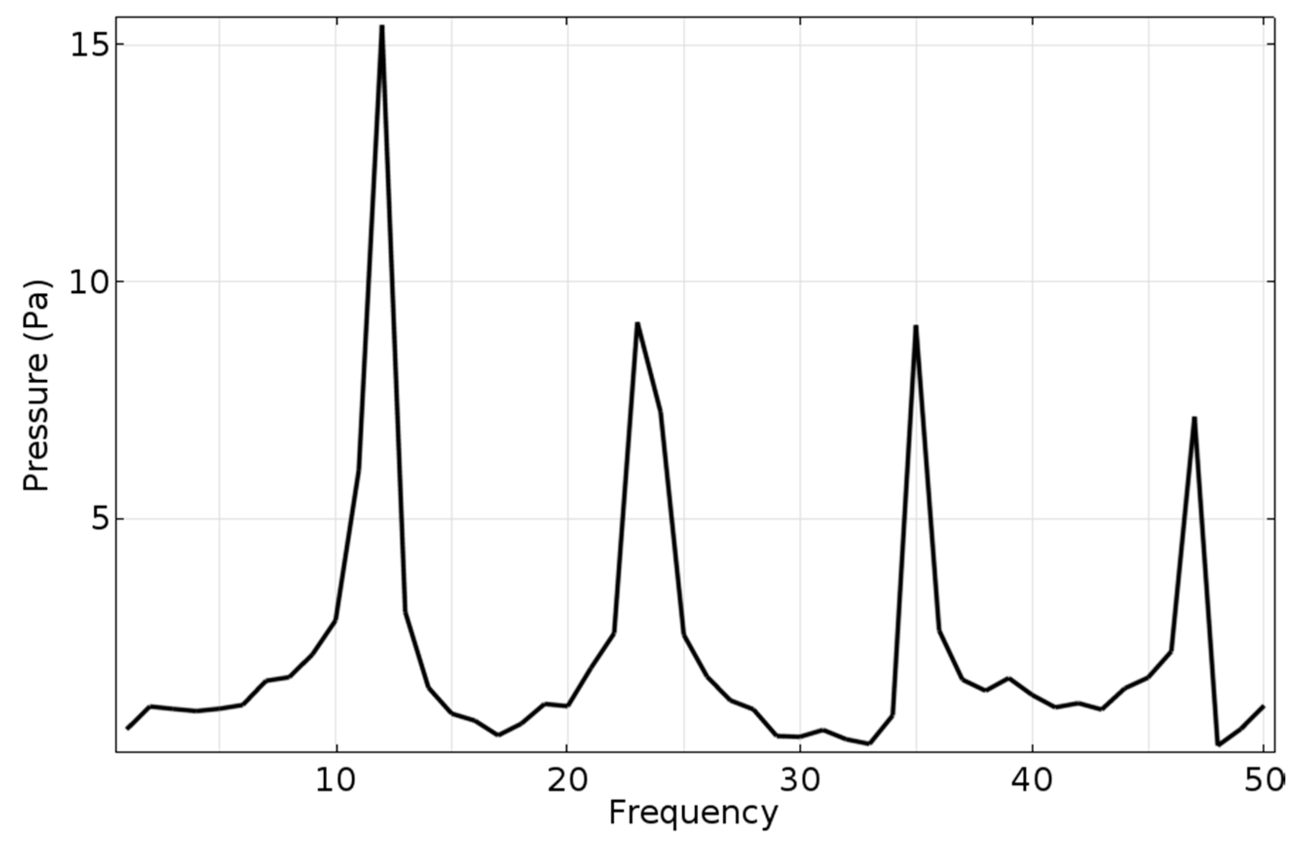
37]. The bubble frequency (dynamic gas pressure at the nozzle) was chosen as the critical variable ( φ 1 = 12 [1/s], φ 2 =10 [1/s] and φ 3 = 9.8 [1/s]). Table 1 presents convergence parameters calculated from the gathered information of the three studies. The verification of the numerical model using a global variable such as the bubble frequency shows that the mesh resolution is appropriated based on the value of the GCI computed. It is desirable that the GCI value would be as low as possible to ensure that the numerical solution will not change with further refinement of the mesh. A GCI value of 6.4% is small and the results are likely to approach to the asymptotic range of convergence. Then, it is expected that further refinement does not substantially change the tracking of the interfaces. However, the presence of discontinuities or singularities can complicate grid convergences studies with the GCI approach [37]. In this study, the singularities arise when the bubble neck’s pinch-off (a finite time singularity in the flow where pressure, velocity, and curvature diverge), consequently this gives non-conservative estimates of discretization errors since the convergence condition ( R ) [38] corresponds to divergence with R = ε 21 / ε 32 = 10 , where ε 21 = ϕ 2 ϕ 1 and ε 32 = ϕ 3 ϕ 2 . Despite that a divergence condition was obtained because of the singularities arising in the study, the verification of numerical accuracy was considered acceptable based on the GCI value and the extrapolated critical variable value ( φ e x t 21 = 12.61   [ 1 / s ] ). The study was also validated by comparing the numerical values of the bubble frequency against those predicted by the analytical equation reported in [25].

3. Results and Discussions

3.1. Bubble Formation Process from an Orifice Embedded in Water and Rise Behavior of Air Bubbles

Most CFD studies that analyze the flow structure in the gas injection have mainly focused in the bubble formation stages: expansion, detachment, deformation, and rise behavior, without including the interaction of the gas bubbles with the free surface at the same time. Only a few works include the interaction of the gas bubbles with the upper interface [24,25].
In this work, the CLSM [19] was employed to simulate the bottom gas injection operation. The aim is to examine the accuracy and capability of this approach to simulate complex problems. The numerical description of these problems is challenging due to the necessity of addressing at the same time many facets of the physical behavior in a high level of detail, requiring a method that can handle complex deformation and motion at the air-liquid interface. For the present case, the numerical solution obtained with the CLSM was assessed quantitatively and qualitatively by comparing the solution against the numerical results reported by [25] using the VOF method. The behavior predicted for the interaction of the two first bubbles formed with the upper air-water interface by both the VOF and LS methods was different under the same operating conditions (physical problem). Therefore, to investigate these differences, the bottom gas injection process in small scale was physically simulated and photographed with a high-speed video camera (720 frames/s), and then the images corresponding to the free surface were compared with the images obtained numerically.
Figure 2 shows the initial stage for the gas injection into quiescent water. There, the bubble is formed whilst attached to the nozzle as the air flows at a constant gas flow rate. Initially, the moment of gas is balanced by the surface tension force, and then the bubble attains a semispherical shape. As the gas enters, the bubble increases its size, and buoyancy forces become important. Then, for a certain volume, the bubble naturally tends to minimize its surface area until the tension in its two surfaces is countered by the excess pressure according to Laplace’s Equation. As a result of this surface minimization, longitudinal curvature changes sign on the base of the bubble, causing the formation of a neck. The incoming gas flux and the buoyancy effect leads to a thinning of this neck until the pinch-off occurs. The pinch-off occurs in two steps. After the formation of a long connecting filament, pinch-off occurs by the retraction of the bubble´s tail and, as the filament is sufficiently elongated, it creates a satellite bubble, which coalesces almost immediately with the former bubble because it is immersed in the former bubble´s wake. Afterwards, the first bubble was released leaving a residual bubble at the nozzle tip, the residual bubble grows up by the same process and eventually a column of discrete bubbles is formed, triggering the liquid flow. This liquid flow, in turn, could facilitate the bubble formation or the detachment of the bubble due to the liquid recirculation motion, which exhibits the highest velocity in the middle plane. However, the velocity at which the surrounding liquid flows near the orifice does not modify the expansion bubble stage, initially established.
A comparison between both the VOF method [25] and the CLSM shows generally good agreement in terms of bubble rise velocities. The maximum bubble rise velocities calculated from each method were very similar, 0.311 m/s for the VOF method and 0.3058 m/s for the LS method. The maximum rise velocity is computed using Equation (12).
w ¯ = 2 π δ w d A δ d A
where w is the velocity in z-direction and A is the area that corresponds to the domain where water is contained. However, differences were found in the shapes that the bubbles undergo in the dynamics of pinch-off and when the bubbles rise, in the bubble formation frequency as well as in the bubble bursting. Bubble sizes after detachment from the orifice were determined in the order of 8.5 mm and of 9.7 mm with the VOF method and LS method, respectively. Figure 3 shows the bubble size obtained with the LS method. The bubble size is an important issue in the gas injection in the context of phenomena related to the bubble’s drag, such as interfacial mass transfer and heat transfer. Theoretically, the bubble diameter should be of the order of 6 mm. Bigger bubbles and faster rise velocities were obtained numerically in both methods due to the wall adhesion’s effect considered in the simulations. For the air-water system studied, a static contact angle of θ a = 110 ° was imposed. This implies low wall wettability, meaning that the injected gas spreads over a larger area around the nozzle. Contrary to non-wetting systems, where the gas does not spread along the wall and for which the theoretical equation holds d B l = 0.794 d o r 0.8 u o r 0.4 , Equation (10) in [25] is used to compute the bubble diameter. This equation assumes that the bubble volume at detachment is controlled principally by the nozzle radii because the bubble base remains attached to the orifice. This explains why simulated bubbles are larger than the theoretical ones. The difference between the bubble sizes obtained with the VOF method and LS method is about 12%.
For the bubble formation frequency, the VOF method [25] predicts a bubble frequency of 10 (1/s), while to the CLSM the bubble formation frequency was of 12 (1/s), as shown in Figure 4. The numerical bubble frequency was computed by performing a Fourier analysis of the pressure pulsations of the gas at the exit of the nozzle. The theoretical value of the frequency of bubble formation under the conditions studied is 12.2 (1/s). A comparison between the theoretical and numerical results of frequency of bubble formation shows that the CLSM is more accurate than the VOF method to reproduce the bubble formation frequency, with a relative error lower than 2%. If the numerical bubble frequency is compared against the extrapolated bubble frequency from the verification study 12.61 (1/s), the relative error ( e e x t 21 × 100 % ) is lower than 5%, which shows that the results are in the asymptotic range of convergence. The bubble formation is considered to take place in the dynamic regime according to Mccann and Prince [39] since the flow rate used in this study is near to 3.93 × 10 6 m3/s. At this flow rate, the bubble formation is governed by the interplay of surface tension, buoyancy, viscous and inertial forces. Based on the accuracy of the reproduced frequency of bubble formation, it could be said that the CLSM balances well these forces locally very well during the bubble formation stage; however, this is not true because in the pinch-off event a nonphysical satellite bubble is formed. In the dynamic regime, the bubble formation is not dominated at all by capillary forces. Capillary forces are more important at the gas flow rate < 0.167 × 10 6 m3/s [39]. However, as can be seen, the entropy condition in the level set equation for the vanishing viscosity (R.H.S. of Equation (11)) implemented in the method to propagate the interface, plays an important role in predicting gradual variations of the surface tension force even for regimes not dominated by capillary forces. This results in a stable local balance of the forces involved in the bubble formation in the Navier-Stokes equation. During the gas injection, the frequency of bubble formation must be appropriately reproduced to consider the collective effects of bubbles, taking into account that the bubble´s wake can influence the ascent velocity of the subsequent bubbles.
In this work, during the bubble formation stage, it was found that the CLSM suffers from the drawback that it predicts the formation of nonphysical satellite bubbles in the pinch-off dynamics of bubbles. The pinch-off process can be characterized by the mass density ratio D = ρ g / ρ l (mathematical model written in the dimensionless form [40]), whereas, for systems of low-density bubble surrounded by a dense fluid, such as air rising in water, D 0 and it corresponds to the pinch-off of bubbles surrounded by inviscid liquids. When D 0 , the creation of satellite bubbles is not expected physically and the point of separation exhibits symmetry in the vertical direction and the neck radius undergoes a sudden rupture [40]. Contrary to the VOF method, with the CLSM, the symmetry in the vertical direction of the point of rupture is lost as the neck radius shrinks before it undergoes a sudden rupture (Figure 5). A possible explanation to this drawback of the simulation may be attributed to the reinitialization parameter needed to track the interface dynamics of the overall process (bubble formation and bubble-free surface interaction), which causes the interface to move slightly in a nonphysical manner. Gas velocity varies abruptly in the bubble’s neck during bubble formation stage since the neck’s bubble is attached to the gas source, thus surface tension acts only in the tangential direction on the interface in a finite time. This slight motion of the interface in the axial direction results in the formation of long filaments. These filaments will cause the subsequent formation of nonphysical satellite bubbles due to the capillary waves in the filament surface. Figure 6 shows the variation in the superficial gas velocity inside the bubble, while this is attached to the nozzle. The abrupt change in the velocity at that instant is explained by the relation u 1 A 1 = u 2 A 2 , since the flow rate is constant. Gas velocity varies to almost 5 times the inlet velocity (0.2 m/s) by reaching a maximum velocity of 0.98 m/s when bubbles are formed.
It is well known that the bubble behavior during its rise depends considerably on the bubble diameter, which is influenced strongly by the nozzle diameter. In order to obtain a bubble diameter as precise as possible, a fine grid spanning the nozzle radius and in the nozzle neighborhood is desired to compute correctly the moving contact line at the wetted wall, during the bubble formation. In the bubble rise, the CLSM shows that it can satisfactorily describe the bubble rise dynamics because the wobbling of the bubbles was observed (Figure 7) as expected theoretically. According to the bubble regime map of Clift et al. [41], an E o b = 9.8 (Eötvös number, E o b = g Δ ρ d B 2 / σ ) and a Re b = 2000 (bubble Reynolds number, Re b = ρ g u B d B / μ g ) computed numerically for the current operation conditions, an intermediate spherical cap + wobbling regime is shown. In the results computed with the VOF method, the wobbling effect is not observed, only the spherical cap regime, as can be seen in Figure 3 and Figure 5 shown in [25]. As the wobbling effect is expected theoretically, and this phenomenon is strongly influenced by the bubble diameter and the local balance of the forces around the bubble rise, it is shown that the results of the CLSM for the bubble diameter are more accurate than the results of the VOF method.
Figure 7 shows the evolution in the bubble’s shapes at the first stages after the injection began, and at the end of the period studied. The bubbles retain a mainly spherical cap shape, but the wobbling effect is present essentially for all the rising time. This effect appears especially when the bubble has just detached from the orifice due to the retraction of the bubble´s tail. The bubble wobbling effect appears under a rapid change of forces around the bubble interface, which makes the shape of the bubble oscillate as the bubble rises. In order to capture numerically the bubble wobbling effect, the model to track the position of the interface must solve properly the local balance of the forces around the rising bubble. The forces which principally influence the shapes that the bubble undergoes as they rise are the shear imposed by the surrounding liquid and the surface tension, which are well balanced by the CLSM during the bubble rise stage.
Mass conservation is an important issue in the LS method, since this method is prone to gain or lose the mass of the fluids during the simulation. Moreover, mass conservation in the two-phase flow simulations is a criterion related to the correctness of the numerical results. A numerical study [19] shows that the CLSM has the ability to track the interface between the gas and the liquid in a benchmark test such as the rotating circle, vortex test, rising bubble and falling droplet, showing that the surface tension calculation is accurate and relatively easy with very good mass conservation. We examine the evolution of total mass conservation with time, which is shown in Figure 8. The mass per unit volume of gas is plotted against the time to track the mass lost during the simulation. In Figure 8 it can be seen that mass loss is small, 0.018325 g / cm 3 , whereas the volume corresponds to the whole computational domain (revolved), which shows that mass conservation is satisfied.

3.2. Gas Bubble Impingement at the Free Surface

When gas bubbles passage continuously through a free surface and they burst, the process is often accompanied by jets shooting up. After jets reach their peak height and fall due to gravity, they induce oscillations on the free surface, causing its deformation by the wave propagation. Thus, the dynamics of the free surface on this stage produces the formation of droplets by jets of drops and the bursting of the gas bubble. This phenomenon finds an important role in the gas injection process in the context of mass transfer rates across the liquid-gas interface, for example, the gases from the environment are considered as contaminants. The evolution of the free surface undergoes complex deformation due to the continuous propagation of the wave caused by the periodic bubble passage. A simulation that includes the physical description of this phenomenon in a high level of detail makes the numerical problem stiff. As the bubble size is reduced, smaller time steps are necessary, especially when explicit methods are used. The size of the bubbles can be reduced when they interact with a free surface in motion. The gas bubble can experience stages such as ring bubbles or even small gas bubbles that are produced by gas entrapment from the environment. Adaptive meshing such that the grid can be refined close to the interface and adaptive time-stepping can be employed to better resolve fine scale features in the gas-liquid interface. Using adaptive meshing and adaptive time-stepping, solvers may meet a CFL condition where the numerical waves propagate at least as fast as the physical waves. However, in this work, a fixed mesh with non-uniform elements and adaptive time-stepping were employed. Regarding the maximum height deformation of the free surface water-liquid interface when the jet of liquid is formed, the VOF method computed a maximum height of 12.3 (mm), but the jet of liquid is poorly formed, as can be observed in Figure 3 shown in [25]. To the CLSM, the maximum height was 13 (mm), with a jet of liquid clearly formed (Figure 9) due to the surface tension force playing the principal role in this stage, and the LS method poses the ability to handle flows with a strong surface tension. At this time, the jet decays without releasing any jet drops. However, at other times, the bursting of the bubble leads to the production of droplets formed by the collapse of the bubble cavity when the surface wave converges axially, as shown in Figure 10a, and droplets are formed by the rupture of the thin film of liquid above the bubble caused by the capillary instability, such as in Figure 10b. Both values of the maximum height of the jet computed with the VOF and LS method are closer quantitatively. Besides, the propagation of the wave over the free surface renders, in essence, the same behavior in both methods. A more detailed description of the events involved when gas bubbles passage continuously through a free surface is observed in the results of the LS method.
Valencia et al. [25] reported that coalescence between the two first bubbles is observed because the first bubble is the slowest and the second is the fastest. However, the position at which the coalescence occurs is not mentioned. With the LS method, the coalescence of these two bubbles was observed only when coarse meshes were used (coarse and intermediate meshes); moreover, with these meshes, the frequency of bubble formation converges towards that predicted by the VOF method. Therefore, considering that (for this case) similar accuracy pertains between the results of the VOF method and the CLSM when using coarse meshes, coalescence does not occur under such conditions of gas injection because with coarse meshes the results are not in the asymptotic range of convergence as shown in Section 2.2, and the behavior of the free surface is as that simulated by the CLSM. To determine the accuracy of the CLSM to simulate the coalescence of the two first bubbles near the free surface, the gas injection system was physically simulated, and the free surface was pictured using a high-speed camera (720 frames/s). For that purpose, air bubbles in quiescent water were formed in a cylindrical vessel. The gas flow rate is 1.6 × 10 6 m3/s. The radius of the orifice at the bottom is 0.3 mm, and it is placed at the axis of symmetry. The radius of the vessel is 2.5 mm and is initially filled with 5 mm of liquid water. The angle of contact between the liquid and the solid correspond to a polymeric surface, and is θ a = 88 ° . The container is made of a cyclic olefin polymer (COP), which has a roughness low enough that the contact angle hysteresis is negligible. The numerical simulation of this system follows the same numerical procedure as that for the system shown in Figure 1. From the comparison between the physical images and the numerical predictions of the interaction between bubbles coalescing near the free surface (Figure 11), it is straightforward that the behavior experimentally observed is very similar to the behavior predicted by the CLSM. The dynamic of the interface of the bubbles and the free surface predicted by the CLSM shows excellent agreement with the images experimentally obtained. Considering that the exposure of the water to the atmosphere causes surfactant contamination [42] and that the surface tension value can vary between the experiment and the simulation, this may slightly modify the numerical behavior from the physical ones. The results obtained by the numerical model developed using the CLSM to simulate the full process of gas injection demonstrates the efficacy of this approach for describing the moving and deformed interfaces that arise in the gas injection processes.

4. Conclusions

In this work, the capabilities of the CLSM to simulate gas-liquid complex interactions were explored by simulating the bottom gas injection process. Since singularities arise in the study, the divergence condition was obtained in the verification of numerical accuracy, nevertheless, it was considered acceptable since the GCI value was small.
Results were compared with those reported in the literature using the volume of fluid method (VOF), and with those obtained by physically simulating the process to validate the numerical model. The velocity field was obtained numerically and the bubble sizes were very similar between the VOF and CLSM. However, the present study shows that the CLSM presents notable capabilities to simulate accurately the important physical features of the gas injection process.
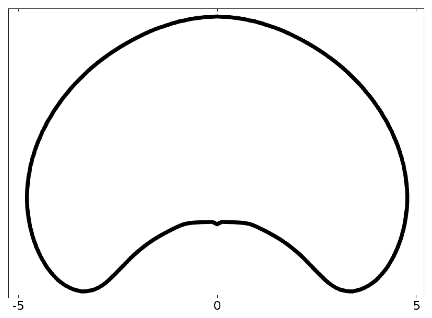
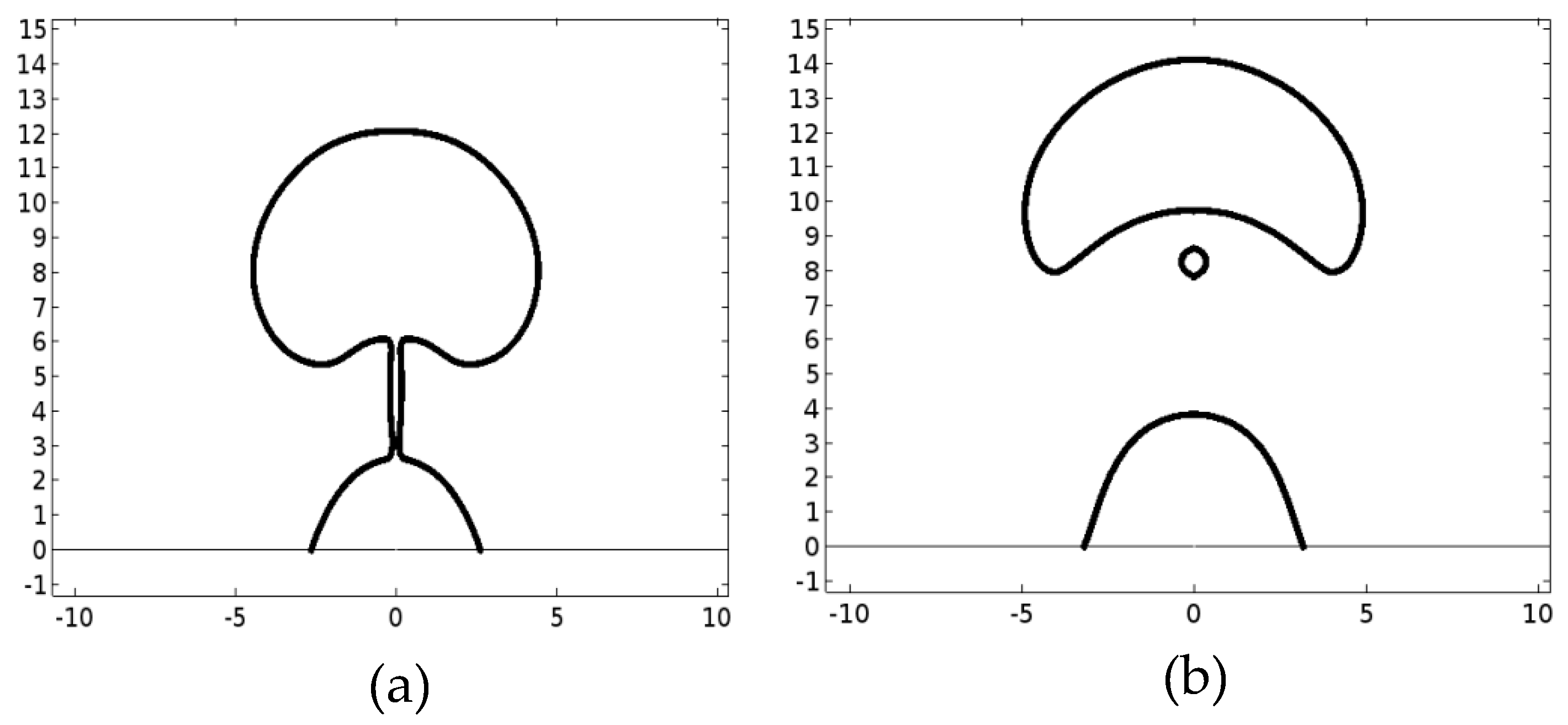
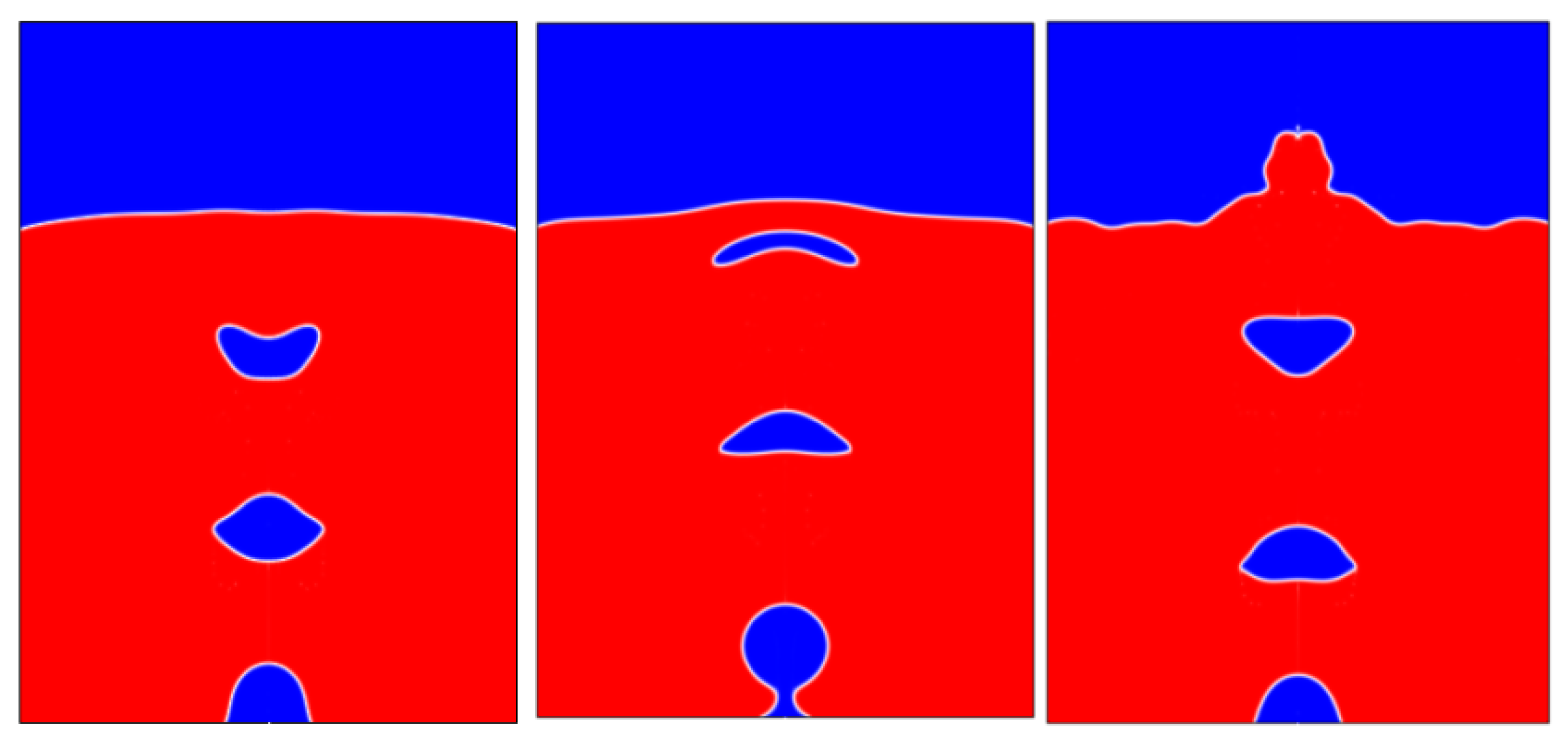
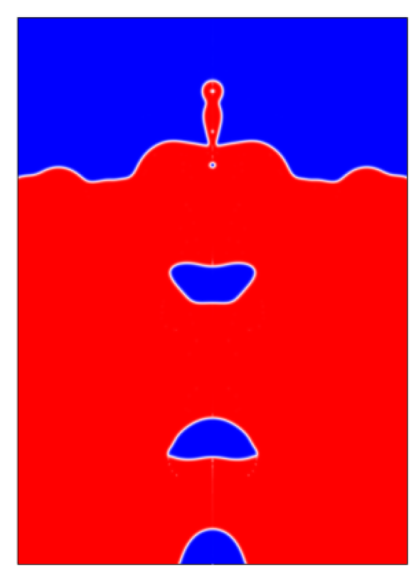
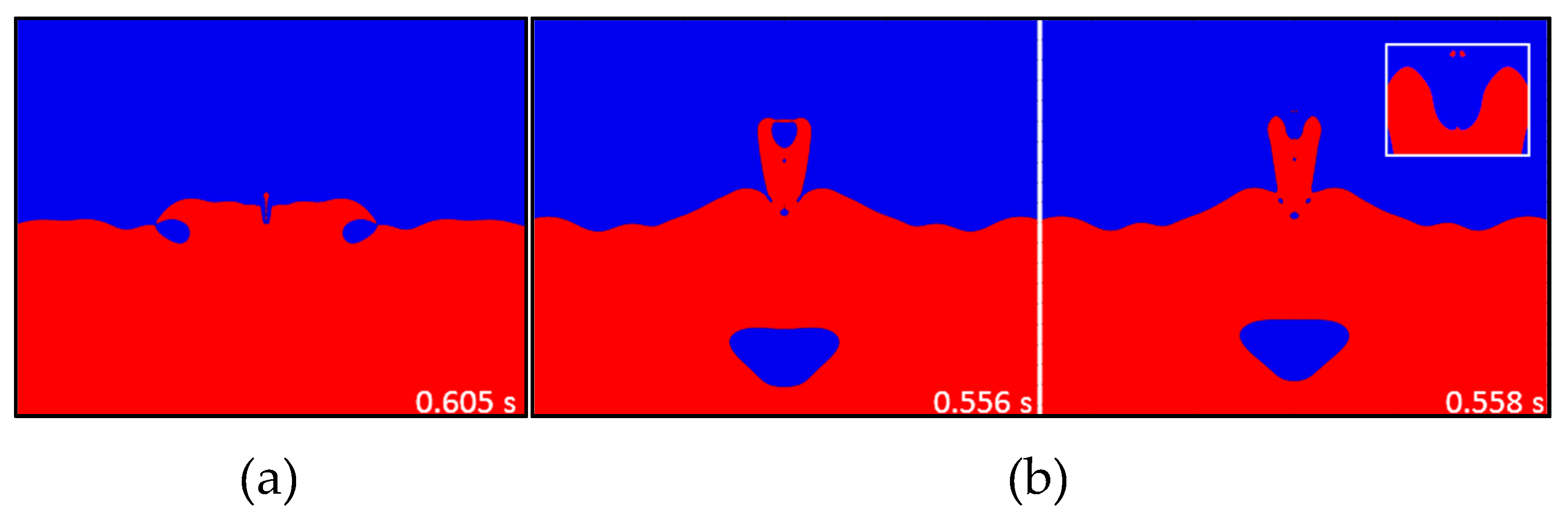
Predictions are accurate even for those regimes where capillary forces do not dominate at all since the LS computes very well the local balance of the forces around the gas-liquid interface. This allows the CLSM to accurately predict the bubble frequency formation and the bubble rise dynamics, as is shown by the complex bubble shapes captured along with the wobbling effect, which was theoretically expected. It was found that the CLSM suffers from the drawback that it predicts the formation of nonphysical satellite bubbles in the pinch-off dynamics of bubbles.
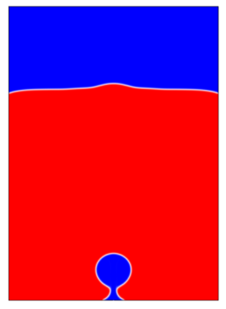
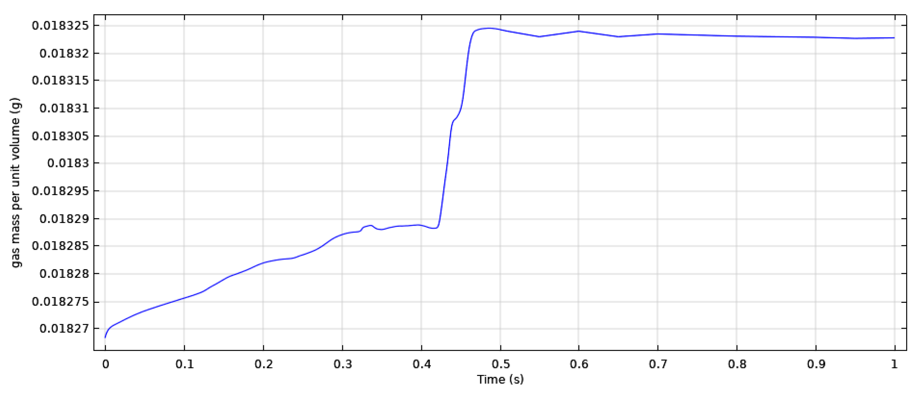
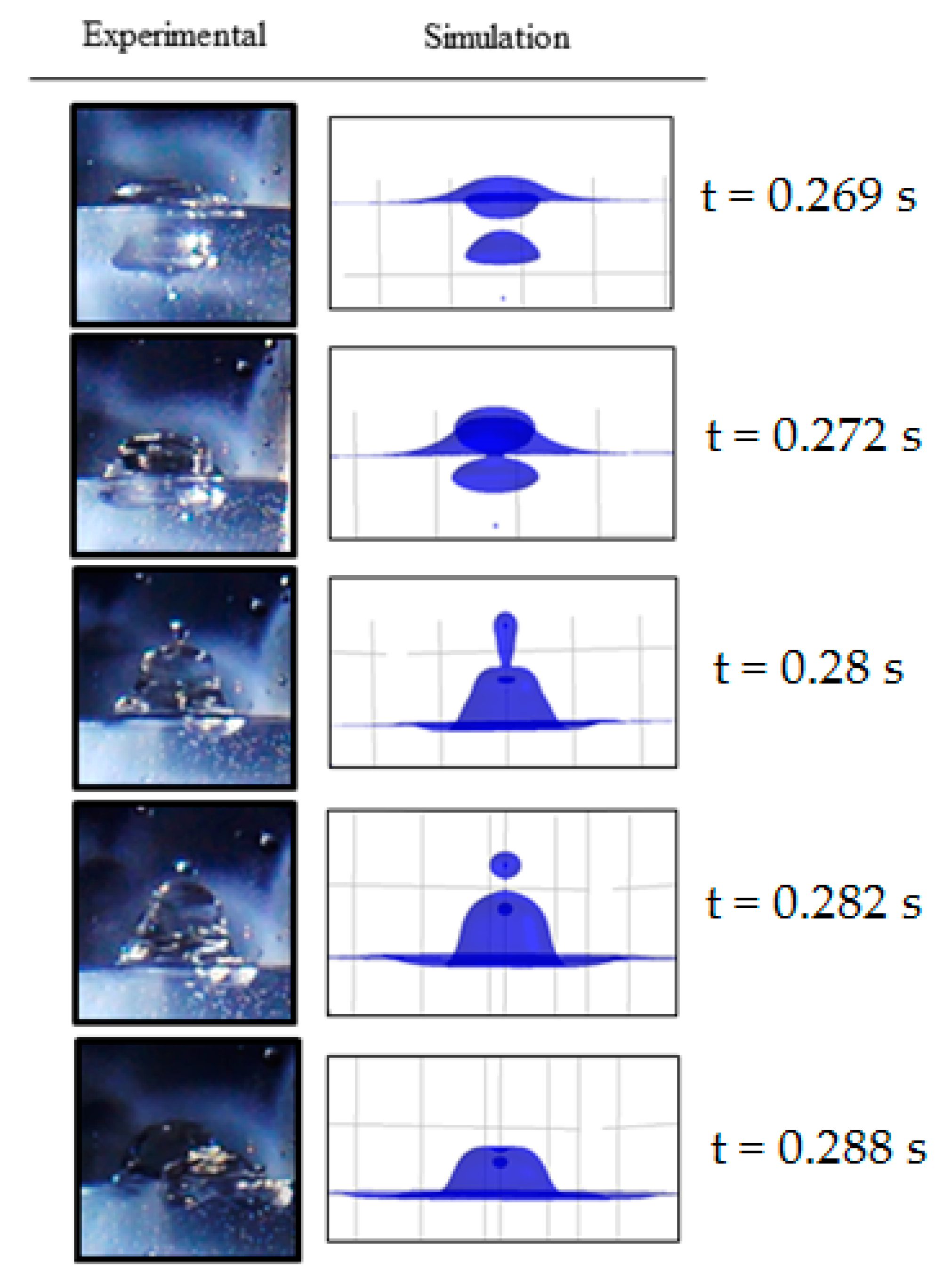
The simulation of the impingement event of the gas bubbles at the free surface compared very well with the physical images obtained in this work. The mass loss is small 0.018325 g / cm 3 showing good mass conservation. Therefore, based on extrapolated and validation errors—5%, and 2% respectively—the CLSM has the accuracy and robustness to capture with a high level of detail the physical phenomena related to gas-liquid complex interactions in fairly complicated systems such as gas injection.

Author Contributions

J.E.R.-S. and K.M.G.-J. designed the study, performed the numerical simulations, and wrote the manuscript; J.E.R.-S. and V.H.G.-P. performed the physical simulation; A.C.-R., resources, J.E.R.-S., K.M.G.-J., V.H.G.-P., A.C.-R., J.A.R.-S., S.L.O.-V., H.A.F.-F. and C.A.Á.-O., funding acquisition. All authors have read and agreed to the published version of the manuscript.

Funding

The APC was funded by the FORDECYT project 296356.

Acknowledgments

The authors wish to thank the Institutions CONACYT, SNI, Centro de Investigación en Química Aplicada, and Instituto Politécnico Nacional, for their permanent support. The authors also kindly acknowledge CONACYT (México) for giving financial support to this work through the FORDECYT project 296356. J.E. Rivera gratefully acknowledges the financial support received from Cátedras CONACYT project 809.

Conflicts of Interest

The authors declare no conflict of interest.

Nomenclature

E o b Eötvös number ( E o b = g Δ ρ d B 2 / σ )
e a 21 approximate relative error
e e x t 21 extrapolated relative error
g gravitational acceleration vector in z-direction (m/s2)
n normal at the interface
p pressure (N/m2)
Re b bubble Reynolds number ( Re b = ρ g u B d B / μ g )
rradial component of the axisymmetric co-ordinate (mm)
r 21 , r 32 intermediate-fine and coarse-intermediate grid refinement factors, respectively
p order of accuracy
t time (s)
u velocity vector ( u , v )
zvertical component of the axisymmetric co-ordinate (mm)
Greek Symbols
δ delta function
ε interface numerical thickness (m)
γ reinitialization of the level set function
κ mean curvature of the interface (m−1)
μ viscosity of mixture (Pa s)
ρ density of mixture (kg/m3)
σ surface tension coefficient (N/m)
ϕ level set function
φ e x t 21 extrapolated value of the critical variable
Subscripts
ggas
lliquid
s t surface tension

References

  1. Hua, J.; Lou, J. Numerical simulation of bubble rising in viscous liquid. J. Comput. Phys. 2007, 222, 769–795. [Google Scholar] [CrossRef]
  2. Zhang, A.; Cui, P.; Cui, J.; Wang, Q. Experimental study on bubble dynamics subject to buoyancy. J. Fluid. Mech. 2015, 776, 137–160. [Google Scholar] [CrossRef] [Green Version]
  3. Ming, F.; Sun, P.; Zhang, A. Numerical investigation of rising bubbles bursting at a free surface through a multiphase SPH model. Meccanica 2017, 52, 2665–2684. [Google Scholar] [CrossRef]
  4. Pinilla, A.; Guerrero, E.; Henao, D.H.; Reyes, D.V.; Pereyra, E.; Soto, G.; Ratkovich, N. CFD modelling of two-phase gas-liquid annular flow in terms of void fraction for vertical down- and up-ward flow. SN Appl. Sci. 2019, 1, 1382. [Google Scholar] [CrossRef] [Green Version]
  5. Chen, X.; Chen, N.; Delgado, A. Numerical study of formation of a series of bubbles at a submerged orifice. Appl. Math. Model. 2019, 73, 668–694. [Google Scholar] [CrossRef]
  6. Åsmund, E. Comment on the level-set method used in ‘Numerical study on mobilization of oil slugs in capillary model with level set approach’. Eng. Appl. Comput. Fluid. Mech. 2016, 10, 466–472. [Google Scholar]
  7. Chen, L.; Garimella, S.; Reizes, J.; Leonardi, E. The Development of a Bubble Rising in a Viscous Liquid. J. Fluid. Mech. 1999, 387, 61–96. [Google Scholar] [CrossRef] [Green Version]
  8. Hirt, C.; Nichols, B. Volume of fluid (VOF) method for the dynamics of free boundaries. J. Comput. Phys. 1981, 39, 201–225. [Google Scholar] [CrossRef]
  9. Osher, S.; Sethian, J. Fronts propagating with curvature-dependent speed: Algorithms based on Hamilton-Jacobi formulations. J. Comput. Phys. 1988, 79, 12–49. [Google Scholar] [CrossRef] [Green Version]
  10. Rider, W.; Kothe, D. Reconstructing volume tracking methods. J. Comput. Phys. 1998, 141, 112–152. [Google Scholar] [CrossRef] [Green Version]
  11. Sussman, M.; Smereka, P.; Osher, S. A level set approach for computing solutions to incompressible two-phase flow. J. Comput. Phys. 1994, 114, 146–159. [Google Scholar] [CrossRef]
  12. Bourlioux, A. Coupled level set volume of fluid algorithm for tracking material interfaces. In Proceedings of the 6th International Symposium on Computational Fluid Dynamics, Lake Tahoe, CA, USA, 4–8 September 1995. [Google Scholar]
  13. Sussman, M.; Puckett, E. A coupled level set and volume of fluid method for computing 3D and axisymmetric incompressible two-phase flows. J. Comput. Phys. 2000, 162, 301–337. [Google Scholar] [CrossRef] [Green Version]
  14. Sussman, M.; Fatemi, E.; Smereka, P.; Osher, S. An improved level set method for incompressible two-phase flows. Comput. Fluids 1998, 27, 663–680. [Google Scholar] [CrossRef]
  15. Herrmann, M. Refined level set grid method for tracking interfaces. In CTR Annual Research Briefs; Center for Turbulence Research: Stanford, CA, USA, 2005; pp. 3–18. [Google Scholar]
  16. Herrmann, M. A balanced force refined level set grid method for two-phase flows on unstructured flow solver grids. J. Comput. Phys. 2008, 227, 2674–2706. [Google Scholar] [CrossRef]
  17. Olsson, E.; Kreiss, G. A conservative level set method for two-phase flow. J. Comput. Phys. 2005, 210, 225–246. [Google Scholar] [CrossRef]
  18. Wang, Y.; Simakhina, S.; Sussman, M. A hybrid level set-volume constraint method for incompressible two-phase flow. J. Comput. Phys. 2012, 231, 6438–6471. [Google Scholar] [CrossRef]
  19. Olsson, E.; Kreiss, G.; Zahedi, S. A conservative level set method for two-phase flow II. J. Comput. Phys. 2007, 225, 785–807. [Google Scholar] [CrossRef]
  20. Albadawi, A.; Donoghue, D.; Robinson, A.; Murray, D.; Delauré, Y. On the analysis of bubble growth and detachment at low Capillary and Bond numbers using Volume of Fluid and Level Set methods. Chem. Eng. Sci. 2013, 90, 77–91. [Google Scholar] [CrossRef]
  21. Gollakota, A.; Kishore, N. CFD study on rise and deformation characteristics of buoyancy-driven spheroid bubbles in stagnant Carreau model non-Newtonian fluids. Theor. Comput. Fluid Dyn. 2018, 32, 35–46. [Google Scholar] [CrossRef]
  22. Shervani-Tabar, N.; Vasilyev, O.V. Stabilized conservative level set method. J. Comput. Phys. 2018, 375, 1033–1044. [Google Scholar] [CrossRef]
  23. Sajid, M.; Bennacer, R. Simulation of Single Bubble Dynamics in Nucleate Pool Boiling Using a Conservative Level Set Method. In Proceedings of the ASME 2009 Heat Transfer Summer Conference, San Francisco, CA, USA, 19–23 July 2009. [Google Scholar]
  24. Chen, C.; Liang-Shih, F. Discrete Simulation of Gas-Liquid Bubble Columns and Gas-Liquid-Solid Fluidized Beds. AIChE J. 2004, 50, 288–301. [Google Scholar] [CrossRef]
  25. Valencia, A.; Cordova, M.; Ortega, J. Numerical simulation of gas bubbles formation at a submerged orifice in a liquid. Int. Commun. Heat Mass. Transf. 2002, 29, 821–830. [Google Scholar] [CrossRef]
  26. Zhang, C.; Fakhari, A.; Li, J.; Luo, L.; Qian, T. A comparative study of interface-conforming ALE-FE scheme and diffuse interface AMR-LB scheme for interfacial dynamics. J. Comput. Phys. 2019, 395, 602–619. [Google Scholar] [CrossRef]
  27. Carlson, A.; Kudinov, P.; Narayanan, C. Prediction of two-phase flow in small tubes: A systematic comparison of state-of-the-art CMFD codes. In Proceedings of the Fifth European Thermal-Sciences Conference, Eindhoven, The Netherlands, 18–22 May 2008. [Google Scholar]
  28. Bai, F.; Han, D.; He, X.; Yang, X. Deformation and coalescence of ferrodroplets in Rosensweig model using the phase field and modified level set approaches under uniform magnetic fields. Commun. Nonlinear. Sci. Numer. Simulat. 2020, 85, 1–23. [Google Scholar] [CrossRef]
  29. Amiri, H.; Hamouda, A. Evaluation of level set and phase field methods in modeling two phase flow with viscosity contrast through dual-permeability porous medium. Int. J. Multiphas. Flow 2013, 52, 22–34. [Google Scholar] [CrossRef]
  30. Labarca, M.; González, J.; Araujo, C. Computational and Experimental Fluid Mechanics with Applications to Physics, Engineering and the Environment, Feasibility of Slug Flow Simulation Using the Commercial Code CFX; Springer International Publishing: Cham, Switzerland, 2014; pp. 379–387. [Google Scholar]
  31. Oshaghi, M.; Afshin, H.; Firoozabadi, B. Investigation of bubble formation and its detachment in shear-thinning liquids at low capillary and Bond numbers. Theor. Comput. Fluid. Dyn. 2019, 33, 463–480. [Google Scholar] [CrossRef]
  32. Lafaurie, B.; Nardone, C.; Scardovelli, R.; Zaleski, S.; Zanetti, G. Modelling merging and fragmentation in multiphase flows with surfer. J. Comput. Phys. 1994, 113, 134–147. [Google Scholar] [CrossRef]
  33. COMSOL. COMSOL Multiphysics CFD Module User’s Guide, Version 5.2a; COMSOL Inc.: Stockholm, Sweeden, 2016. [Google Scholar]
  34. Brooks, A.; Hughes, T. Streamline upwind/Petrov-Galerkin formulations for convection dominated flows with particular emphasis on the incompressible Navier-Stokes equations. Comput. Methods Appl. Mech. Eng. 1982, 32, 199–259. [Google Scholar] [CrossRef]
  35. Hughes, T.; Franca, L. A new finite element formulation for computational fluid dynamics: V. Circumventing the Babuska-Brezzi condition: A stable Petrov-Galerkin formulation of the Stokes problem accommodating equal-order interpolations. Comput. Methods. Appl. Mech. Eng. 1986, 59, 85–99. [Google Scholar] [CrossRef]
  36. ASME. Standard for Verification and Validation in Computational Fluid Dynamics and Heat Transfer; The American Society of Mechanical Engineers: New York, NY, USA, 2009; ISBN 9780791832097. [Google Scholar]
  37. Roche, P. Perspective: A Method for Uniform Reporting of Grid Refinement Studies. ASME J. Fluids. Eng. 1994, 116, 405–413. [Google Scholar] [CrossRef]
  38. Stern, F.; Wilson, R.; Coleman, H.; Paterson, E.G. Comprehensive Approach to Verification and Validation of CFD Simulations—Part1: Methodology and Procedures. ASME J. Fluids Eng. 2001, 123, 793–802. [Google Scholar] [CrossRef]
  39. Mccann, D.; Prince, R. Regimes of bubbling at a submerged orifice. Chem. Eng. Sci. 1971, 268, 1505–1512. [Google Scholar] [CrossRef]
  40. Burton, J.; Taborek, P. Bifurcation from bubble to droplet behavior in inviscid pinch-off. Phys. Rev. Lett. 2008, 101, 1–4. [Google Scholar] [CrossRef] [PubMed] [Green Version]
  41. Clift, R.; Grace, J.; Weber, M. Bubbles, Drops and Particles; Academic Press: New York, NY, USA, 1978; p. 27. ISBN 012176950X. [Google Scholar]
  42. Kelsall, G.; Tang, S.; Smith, A.; Yurdakul, S. Measurement of rise and electrophoretic velocities gas bubbles. J. Chem. Soc. Faraday Trans. 1996, 92, 3879–3893. [Google Scholar] [CrossRef]
Figure 1. Schematic diagram of the bottom gas injection process with dimensions in millimeters mm (the orifice diameter is 5.0 mm) (a), and boundary conditions (b).
Processes 08 01643 g001
Figure 2. Bubble formed on a low wetting surface at a time of 0.091 s.
Processes 08 01643 g002
Figure 3. Bubble diameter after detachment from the orifice computed with the level set method (9.7 mm).
Processes 08 01643 g003
Figure 4. Fourier transformation of the dynamic pressure at the nozzle.
Processes 08 01643 g004
Figure 5. The pinch-off dynamic of the bubble. (a) The connecting filament elongated (0.096 s). (b) Satellite bubble formed (0.106 s).
Processes 08 01643 g005
Figure 6. Velocity field after 0.34 s of gas injection. The short red lines represents some velocity vectors.
Processes 08 01643 g006
Figure 7. Evolution of the shapes of the bubbles after 0.22, 0.26, 0.9 s injection time.
Processes 08 01643 g007
Figure 8. Loss of gas mass during the simulation.
Processes 08 01643 g008
Figure 9. The jet of liquid produced when bubbles break through the free surface after 0.392 s.
Processes 08 01643 g009
Figure 10. Droplets produced by the bubble bursting process. The collapse of the bubble cavity (a) and rupture of the film of liquid (b).
Processes 08 01643 g010
Figure 11. The sequence of the deformation of the air-water free surface by the impingement of two bubbles coalescing while rising to the free surface. The 3D numerical images were obtained by revolving the ϕ variable around the symmetry axis.
Processes 08 01643 g011
Table 1. Calculation of Grid Convergence Index.
φ = Bubble   Frequency ( 1 / s )
N 1 , N 2 , N 3 175,202, 21,196, 5900
r 21 2.875
r 32 1.89
φ 1 12
φ 2 10
φ 3 9.8
p 1.37
φ e x t 21 12.61
e a 21 0.1666
e e x t 21 0.0483
G C I fine   mesh   solution 21 6.4%
Publisher’s Note: MDPI stays neutral with regard to jurisdictional claims in published maps and institutional affiliations.

