Optimization of an Inter-Plant Hydrogen Network: A Simultaneous Approach to Solving Multi-Period Optimization Problems

Abstract

Inter-plant hydrogen integration can reduce the consumption of hydrogen utility in petrochemical parks. However, the fluctuation of operating conditions will lead to complex multi-period problems of hydrogen network integration. This work develops a simultaneous optimization approach to solving multi-period optimization problems for the inter-plant hydrogen network. To do this, we consider the inter-plant hydrogen integration and the fluctuation of operating conditions in each plant at the same time, and aim to minimize the total annualized cost of the entire hydrogen system of all plants involved. An industrial case study of a three-plant hydrogen network with seven subperiods was adopted to verify the effectiveness of the proposed method. Results show that the optimal structure and the corresponding scheduling scheme can be obtained when the lowest cost of the system is targeted. Compared with the stepwise methods, the proposed approach features taking the characteristics of all subperiods into account simultaneously and making the structure of the hydrogen network much more effective and economical. For the scheduling schemes, the utilization efficiency of the internal hydrogen sources is increased by hydrogen exchange among the plants.

1. Introduction

Chemical industry parks generally consist of companies that produce a variety of chemical products, where hydrogen is usually used as a utility [1]. The integration of the hydrogen network is an effective approach to optimize the allocation of hydrogen utility and reduce operation costs [2]. In these parks, the quantity and quality of hydrogen supply and demand in each company are usually different, which makes it possible to integrate the hydrogen networks for all plants [3]. Comparing to integrating the hydrogen network in a single plant, integrating hydrogen systems for multiple plants could further reduce utility consumption and improve the utilization efficiency of hydrogen by allowing the transportation of hydrogen streams across plants [4]. Nevertheless, the supply and demand of hydrogen in the plants change over time, and the flowrates fluctuation in one plant does not synchronize with the other one. Therefore, to make the best use of the hydrogen utilities in the chemical industry parks, multi-period methods are often adopted to optimize the holistic hydrogen network by considering the varying operating conditions of the hydrogen streams in the whole park.

For the multi-period method applied in the optimization of the hydrogen network, the operating duration is usually divided into several subperiods to approximate the fluctuations of the operating conditions, and the operational parameters are kept constant in each subperiod. Liang et al. [5] presented a multi-period optimization model for the hydrogen network and investigated the influences of the number and the duration of subperiods on the optimal design of the hydrogen network. The solution strategies for the optimization of multi-period hydrogen network can be categorized into two kinds of methods, i.e., stepwise methods and simultaneous methods. For the stepwise strategies, the problem is decomposed into subproblems to reduce the number of model variables, and the final hydrogen network can be obtained by synthesizing the design scheme of each subperiod [6,7,8]. Although the scale of the model is reduced, it is difficult to appraise the performance of the hydrogen network in each subperiod in a comprehensive way. Thus, the hydrogen network structures obtained by the stepwise methods are usually local optima. On the contrary, the simultaneous methods fully consider the trade-off between each subperiod, and the configurations and schedule schemes of the hydrogen network with much better performance can be achieved. Nevertheless, the solution process could be time-consuming [9] when the scale of the model is enlarged [10].

For the inter-plant integration of the hydrogen network, there are basically three ways. The first way is to share the hydrogen utilities by pipelines to directly meet the demands of hydrogen sinks in all plants. The second one is that the purifier is used to increase the purities of some internal hydrogen sources in one plant and deliver them to other plants. The last one is that intermediate hydrogen headers are set up among these plants. Deng et al. [11] realized that integrating the hydrogen systems through hydrogen pipelines and centralized purifiers. In their work, all possible connections of the inter-plant hydrogen network were considered in the superstructure, and the influences of design conditions of the purifiers on the performances were studied comprehensively. Kang et al. [12] integrated the inter-plant hydrogen network through intermediate headers, of which the hydrogen purity and pressure were optimized in turn. Lou et al. [13] synthesize the inter-plant hydrogen network by the cross-plant pipelines and purifiers. In their method, the hydrogen allocation among the plants was optimized by using a transshipment model, and then the intra-plant structure of individual hydrogen networks was designed. Although the abovementioned studies can be used to optimize integrating the inter-plant hydrogen network, the influences of the operating condition fluctuations on the structure and scheduling schemes are somehow ignored. To consider the fluctuations of the operating conditions, Shehata et al. [14] used the results of a single period model to synthesize the multi-period hydrogen network and achieved a significant reduction in operating costs. However, this stepwise approach fails to consider the relationships and trade-offs among subperiods, and the design scheme of the hydrogen system is greatly affected by the worst case, which may cause an unnecessary increase of investment cost in the plants. Therefore, it is necessary to develop a multi-period simultaneous method to realize the optimal design of the inter-plant hydrogen system considering the fluctuations of the operating conditions in all plants.

To address the abovementioned issues, a multi-period simultaneous optimization method for the inter-plant hydrogen system, which features a mixed-integer linear programming (MILP) problem, is proposed to coordinate the supply and demand of hydrogen and realize the lowest total annual cost (TAC) of the hydrogen network in a chemical industry park. In this method, the hydrogen networks in different plants are connected by the hydrogen supply pipeline across the plants and the centralized purifier in each plant. A case study is used to illustrate the effectiveness and advantages of the proposed method.

The rest of this paper is arranged as follows. The problem statement is given in Section 2, followed by introducing the multi-period optimization model of the inter-plant hydrogen network in Section 3. The case study is given in Section 4, and the conclusions are drawn in Section 5.

2. Problem Statement

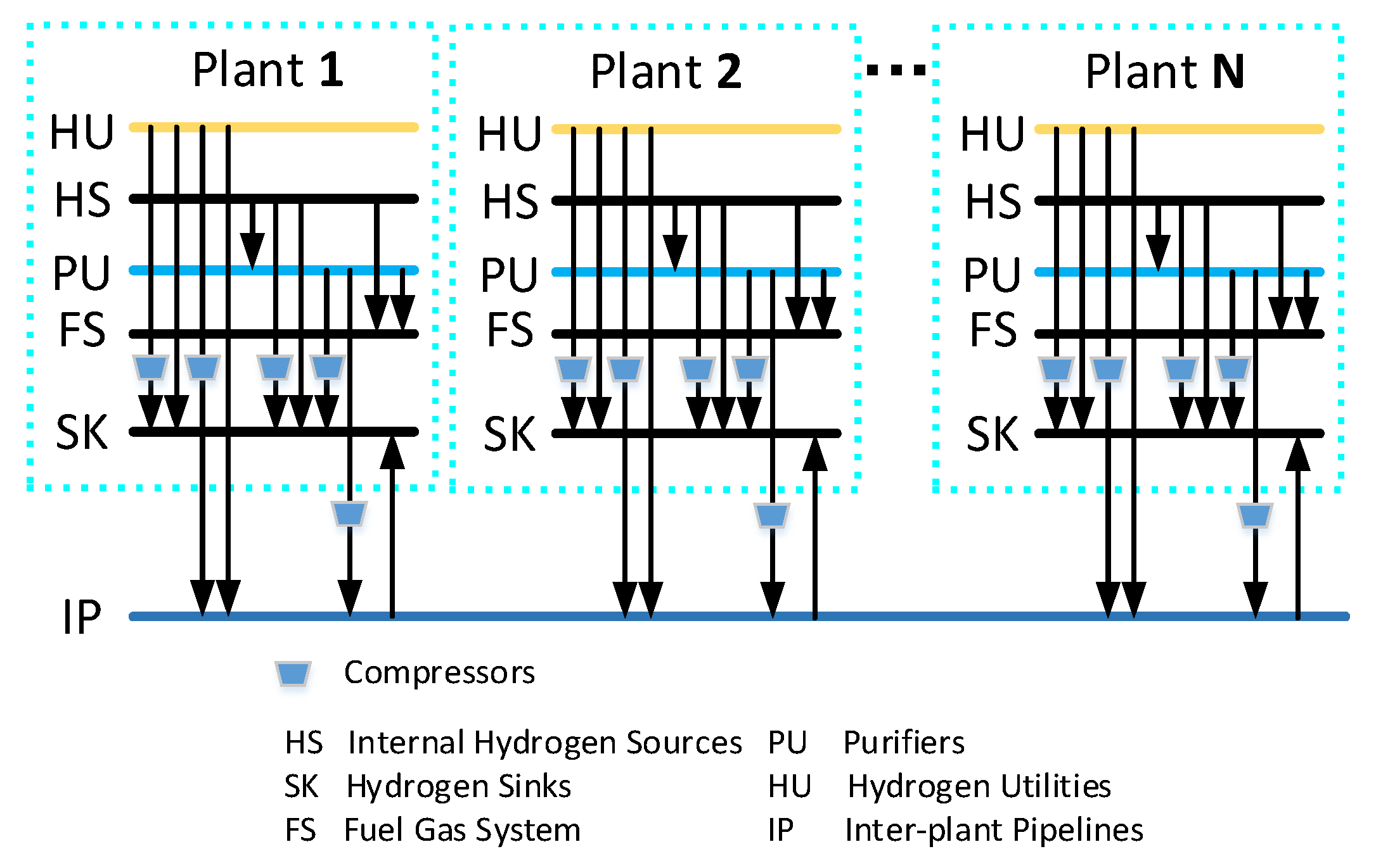
Figure 1 presents the superstructure of the hydrogen system with N plants in a chemical industry park, which is composed of hydrogen sources, hydrogen sinks, purifiers, compressors, intra-plant pipelines, cross-plant pipelines, and a fuel gas system.

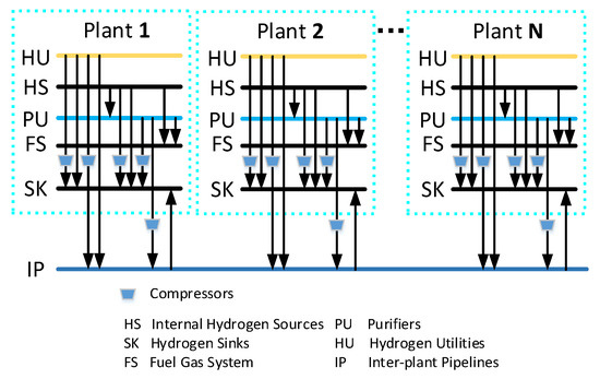
Figure 1. The superstructure of the inter-plant hydrogen network.

The hydrogen sources consist of internal hydrogen sources ($i\in HS$) and hydrogen utilities ($j\in HU$), and the set of all the hydrogen sources in the inter-plant hydrogen network can be expressed as $s\in SC$, $SC=HU\cup HS$. The set of hydrogen–consuming units are denoted as hydrogen sinks ($k\in SK$). The hydrogen utilities can be delivered to the hydrogen sinks within a plant via the intra-plant pipelines, or to hydrogen sinks of other plants via the cross-plant pipelines. The internal hydrogen source can only be delivered to the hydrogen sinks within a plant, or to the purifier as a feed stream, or directly discharged to the fuel gas system. The centralized purifier ($m\in PU$) of each plant only deals with the internal hydrogen source streams from the same plant, and the product stream can be allocated to all hydrogen sinks, and the residual stream is fed to the fuel gas system. The compressors are used to elevate the pressure of the hydrogen streams to meet the inlet requirements of the hydrogen sinks and the purifiers. In the hydrogen network of plant n ($n\in N$), the flowrates, purities, and pressures of hydrogen sources and sinks are known. In addition, the distances among the plants are also known.

The main assumptions are listed as follows.

• A dedicated hydrogen pipeline is set for each cross-plant match;
• In each plant, at most one centralized purifier can be set up;
• A dedicated compressor is placed for each match that needs elevating pressure.

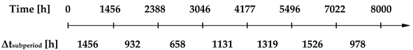
The fluctuations of the hydrogen sources and hydrogen sinks in different plants may change out of synchronization. Hence, for the plants involved, to integrate the hydrogen networks in different plants, the partitioning of subperiod should be carried out in terms of fluctuation of hydrogen sources and sinks throughout the plants, where the operational parameters are kept constant in each subperiod, as shown in Figure 2. In the figure, F_s denotes the flowrate of hydrogen source, and F_k denotes the flowrate of hydrogen sink. The operating time of interest can be divided into p subperiods, in which the flowrates and purities of the hydrogen streams are constant. Then the problem of integrating hydrogen networks in multiple plants is transformed into a multi-period optimization problem of the inter-plant hydrogen network. Moreover, the mathematical programming model needs to be established and solved to obtain the structure of the inter-plant hydrogen network that can accommodate the fluctuating of the hydrogen sources and hydrogen sinks in different plants.

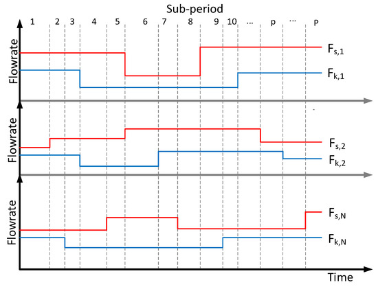
Figure 2. The partitioning of subperiods and flowrates fluctuation of hydrogen sources and hydrogen sinks in different plants. F_s: the flowrate of hydrogen source; F_k: the flowrate of hydrogen sink.

3. Mathematical Programming Model for Multi-Period Optimization of Inter-Plant Hydrogen Networks

3.1. Objective Function

In the model, the hydrogen networks of the three plants are integrated as a whole, where hydrogen utilities are shared among plants and can be transported through cross-plant pipelines to implement the industrial symbiosis. The objective is to minimize the total annual cost (TAC) of the entire hydrogen network in a chemical industry park, which can be formulated as

$$\min TAC=C_{{\mathrm{H}}_2}-C_{\mathrm{fuel}}+C_{\mathrm{ele}}+Af\cdot \left(C_{\mathrm{pur}}+C_{\mathrm{pipe}}+C_{\mathrm{com}}\right)$$

(1)

where $TAC$ is the total annual cost, which is the summation of the operating cost and the capital cost. The operating cost includes the cost of hydrogen utility, $C_{{\mathrm{H}}_2}$, the revenue of fuel gas, $C_{\mathrm{fuel}}$, electricity purchasing cost, $C_{\mathrm{ele}}$; the capital cost includes the purifier cost, $C_{\mathrm{pur}}$, the pipeline cost, $C_{\mathrm{pipe}}$ and the compressor cost, $C_{\mathrm{com}}$.

$Af$ denotes the annualized factor, which is calculated by

$$Af=\frac{fi{(1+fi)}^q}{{(1+fi)}^q-1}$$

(2)

where $fi$ is the annual interest rate, and $q$ is the number of years for depreciation. In this work, $fi$ is 0.05 and $q$ is 5.

The cost of hydrogen utility, $C_{{\mathrm{H}}_2}$, is calculated by

$$C_{{\mathrm{H}}_2}={\displaystyle \sum _{p\in P}\left[t_p\cdot {\displaystyle \sum _{j\in HU}{\displaystyle \sum _{k\in SK}\left(3600\times F_{j,k}^p\cdot e_j\right)}}\right]}$$

(3)

where $t_p$ is the duration of subperiod p, and $e_j$ represents the price of the hydrogen utility. $F_{j,k}^p$ stands for the flowrate supplied from hydrogen utility j to hydrogen sink k under subperiod p.

The revenue of fuel gas, $C_{\mathrm{fuel}}$, is calculated by

$$C_{\mathrm{fuel}}=e_{\mathrm{heat}}\cdot {\displaystyle \sum _{p\in P}3600\times t_p\left\{\begin{array}{l}{\displaystyle \sum _{m\in PU}\left[(1-r_m)\cdot {\displaystyle \sum _{s\in SC}(F_{s,m}^p\cdot y_s^p)}\right]}\cdot \mathsf{\Delta }{H}_{{\mathrm{c},\mathrm{H}}_2}^{\mathsf{\Theta }}+\\ {\displaystyle \sum _{i\in HS}(F_{i,SUR}^p\cdot y_i^p)}\cdot \mathsf{\Delta }{H}_{{\mathrm{c},\mathrm{H}}_2}^{\mathsf{\Theta }}+\\ {\displaystyle \sum _{i\in HS}\left[F_{i,SUR}^p\cdot (1-y_i^p)\right]}\cdot \mathsf{\Delta }{H}_{{\mathrm{c},\mathrm{CH}}_4}^{\mathsf{\Theta }}+\\ {\displaystyle \sum _{m\in PU}\left[F_{m,resd}^p-(1-r_m)\cdot {\displaystyle \sum _{s\in SC}(F_{s,m}^p\cdot y_s^p)}\right]}\cdot \mathsf{\Delta }{H}_{{\mathrm{c},\mathrm{CH}}_4}^{\mathsf{\Theta }}\end{array}\right\}}$$

(4)

where $e_{\mathrm{heat}}$ is the price of heat energy. $r_m$ is the ratio of the flowrate of pure hydrogen in the product stream to that in the feed stream. $F_{s,m}^p$ stands for the flowrate supplied from hydrogen source s to purifier m, and $y_s^p$ denotes the hydrogen purity of hydrogen source s. For the internal hydrogen source i ($i\in HS$), $F_{i,SUR}^p$ is the flowrate allocated to the fuel gas system and $y_i^p$ denotes the hydrogen purity. $F_{m,resd}^p$ denotes the flowrates of the residual stream for purifier m. $\mathsf{\Delta }{H}_{{\mathrm{c},\mathrm{H}}_2}^{\mathsf{\Theta }}$ and $\mathsf{\Delta }{H}_{{\mathrm{c},\mathrm{CH}}_4}^{\mathsf{\Theta }}$ represent the standard combustion heat of hydrogen and methane.

The electricity cost of the compressors can be calculated by

$$C_{\mathrm{ele}}={\displaystyle \sum _{p\in P}{t}_p\cdot e_{\mathrm{ele}}\cdot \left({\displaystyle \sum _{k\in SK}{\displaystyle \sum _{s\in SC}{W}_{s,k}^p}}+{\displaystyle \sum _{m\in PU}{\displaystyle \sum _{s\in SC}{W}_{s,m}^p}}+{\displaystyle \sum _{k\in SK}{\displaystyle \sum _{m\in PU}{W}_{m,k}^p}}\right)}$$

(5)

where $e_{\mathrm{ele}}$ denotes the unit price of electricity.

$W_{a,b}^p$ represents the power of the compressor between supplier a and receiver b in subperiod p [15], which is calculated by

$$\begin{gathered} W_{a,b}^p=z_{a,b}^{p,\mathrm{P}}\cdot F_{a,b}^p\frac{c_{p}T}{\eta }\cdot \left[{\left(\frac{P_b^p}{P_a^p}\right)}^{\frac{\gamma -1}{\gamma }}-1\right] \\ {z}_{a,b}^{p,\mathrm{P}}\in \left\{z_{s,k}^{\mathrm{P}},z_{s,m}^{\mathrm{P}},z_{m,k}^{\mathrm{P}}\right\}\forall s\in SC,m\in PU,k\in SK,p\in P \end{gathered}$$

(6)

where $z_{a,b}^{p,\mathrm{P}}$ is used to judge whether a compressor is necessary to be installed or not; $F_{a,b}^p$ denotes the flowrate from supplier a to receiver b; $c_p$ is the specific heat at constant pressure; $T$ is the inlet temperature and $\eta$ is the efficiency of the compressor; $P_a^p$ and $P_b^p$ are the inlet and outlet pressures of the compressor; $\gamma$ represents the ratio of specific heat.

The capital cost of the pipelines can be estimated by

$$C_{\mathrm{pipe}}={\displaystyle \sum _{k\in SK}{\displaystyle \sum _{s\in SC}{C}_{s,k}}}+{\displaystyle \sum _{m\in PU}{\displaystyle \sum _{s\in SC}{C}_{s,m}}}+{\displaystyle \sum _{k\in SK}{\displaystyle \sum _{m\in PU}{C}_{m,k}}}+{\displaystyle \sum _{i\in HS}{C}_{i,\mathrm{fuel}}}$$

(7)

The capital cost of each pipeline meets the following inequality.

$$\begin{gathered} C_{a,b}\ge \left\{z_{a,b}^p\cdot a_{\mathrm{pipe}}+b_{\mathrm{pipe}}\left[\frac{F_{a,b}^p}{\max (P_a^p,P_b^p)}\right]\right\}\cdot d_{a,b} \\ {C}_{a,b}\in \left\{C_{s,k},C_{s,m},C_{m,k}\right\}\forall s\in SC,m\in PU,k\in SK \\ {z}_{a,b}^p\in \left\{z_{s,k}^p,z_{s,m}^p,z_{m,k}^p\right\}\forall s\in SC,m\in PU,k\in SK,p\in P \end{gathered}$$

(8)

where the binary variable $z_{a,b}^p$ is used to indicate whether the connection between supplier a and receiver b exists in subperiod p. If the flowrate is non-zero, $z_{a,b}^p$ is equal to one, otherwise $z_{a,b}^p$ is zero which means that the connection does not exist. $C_{a,b}$ is the capital cost of the pipeline between supplier a and receiver b; $a_{\mathrm{pipe}}$ and $b_{\mathrm{pipe}}$ are the capital cost coefficients of the pipelines [12]; $d_{a,b}$ represents the distance between supplier a and receiver b.

The capital cost of the pipeline from hydrogen utility i to the fuel gas system is denoted as $C_{i,\mathrm{fuel}}$, which meets the following inequality.

$$C_{i,\mathrm{fuel}}\ge \left[a_{\mathrm{pipe}}\cdot z_{i,\mathrm{fuel}}+b_{\mathrm{pipe}}\cdot \left(\frac{F_{i,SUR}^p}{P_i^p}\right)\right]\cdot d_{i,\mathrm{fuel}}\forall i\in HS,p\in P$$

(9)

where the binary variable $z_{i,\mathrm{fuel}}$ is used to indicate whether the connection from the internal hydrogen source i to the fuel gas system exists or not; $d_{i,\mathrm{fuel}}$ denotes the distance between internal hydrogen source i and the fuel gas system.

The capital cost of the compressors can be expressed as

$$C_{\mathrm{com}}={\displaystyle \sum _{k\in SK}{\displaystyle \sum _{s\in SC}{C}_{s,k}^{\mathrm{P}}}}+{\displaystyle \sum _{m\in PU}{\displaystyle \sum _{s\in SC}{C}_{s,m}^{\mathrm{P}}}}+{\displaystyle \sum _{k\in SK}{\displaystyle \sum _{m\in PU}{C}_{m,k}^{\mathrm{P}}}}$$

(10)

The capital cost of each compressor is denoted as $C_{a,b}^{\mathrm{P}}$, which meets the following inequality.

$$\begin{gathered} C_{a,b}^{\mathrm{P}}\ge C_{a,b}^{p,\mathrm{P}} \\ {C}_{a,b}^{\mathrm{P}}\in \left\{C_{s,k}^{\mathrm{P}},C_{s,m}^{\mathrm{P}},C_{m,k}^{\mathrm{P}}\right\}\forall s\in SC,m\in PU,k\in SK \\ {C}_{a,b}^{p,\mathrm{P}}=\left(a_{\mathrm{com}}\cdot z_{a,b}^p\cdot z_{a,b}^{p,\mathrm{P}}+b_{\mathrm{com}}\cdot W_{a,b}^p\right)\times {10}^4 \\ {z}_{a,b}^p\in \left\{z_{s,k}^p,z_{s,m}^p,z_{m,k}^p\right\}\forall s\in SC,m\in PU,k\in SK,p\in P \end{gathered}$$

(11)

where $C_{a,b}^{p,\mathrm{P}}$ denotes the capital cost of the compressor, which is calculated by its power in subperiod p; $a_{\mathrm{com}}$ and $b_{\mathrm{com}}$ are the capital cost coefficients of the compressors [16].

The required power of the compressor in each subperiod is less than the rated power, given by

$$\begin{gathered} W_{a,b}\ge W_{a,b}^p\forall p\in P \\ {W}_{a,b}\in \left\{W_{s,k},W_{s,m},W_{m,k}\right\}\forall s\in SC,m\in PU,k\in SK \end{gathered}$$

(12)

where $W_{a,b}$ denotes the rated power of the compressor.

The capital cost of the purifiers can be expressed as

$$C_{\mathrm{pur}}={\displaystyle \sum _{m\in PU}{C}_m}$$

(13)

$C_m$ denotes the capital cost of centralized purifier m, which meets the following inequality.

$$\begin{gathered} C_m\ge C_m^p\forall m\in PU,p\in P \\ {C}_m^p=\left(a_{\mathrm{pur}}\cdot z_m+b_{\mathrm{pur}}\cdot F_m^p\right)\times {10}^4\forall m\in PU,p\in P \end{gathered}$$

(14)

where $C_m^p$ stands for the capital cost of centralized purifier m under subperiod p; $a_{\mathrm{pur}}$ and $b_{\mathrm{pur}}$ are the capital cost coefficients of the purifiers [16]; the binary variable $z_m$ is used to indicate whether the purifier m exists or not; $F_m^p$ is the feed flowrate for purifier m in subperiod p.

3.2. Constraints

3.2.1. Constraints of Hydrogen Sources and Hydrogen Sinks

In a certain subperiod, each hydrogen source can be allocated to hydrogen sinks, purifiers, and the fuel gas system. The flowrate balance of the hydrogen source can be formulated as

$$F_s^p={\displaystyle \sum _{k\in SK}{F}_{s,k}^p}+{\displaystyle \sum _{m\in PU}{F}_{s,m}^p}+F_{s,SUR}^p\forall s\in SC,p\in P$$

(15)

where $F_s^p$ is the flowrate of hydrogen source s in subperiod p; $F_{s,k}^p$ stands for the flowrate supplied from hydrogen source s to hydrogen sink k. For the hydrogen utility $j$ ($j\in HU$), $F_{j,SUR}^p$ represents the excessive production capacity.

In subperiod p, hydrogen sources and purifiers should meet the requirement of a hydrogen sink. The flowrate balance of the hydrogen sink can, thus, be expressed as

$$F_k^p={\displaystyle \sum _{s\in SC}{F}_{s,k}^p}+{\displaystyle \sum _{m\in PU}{F}_{m,k}^p}\forall k\in SK,p\in P$$

(16)

where $F_k^p$ represents the flowrate supplied to hydrogen sink k in subperiod p; $F_{m,k}^p$ denotes the flowrate supplied from purifier m to hydrogen sink k.

The flowrate supplied to hydrogen sink k should not be less than the required flowrate, $F_{k,req}^p$, given by

$$F_k^p\ge F_{k,req}^p\forall k\in SK,p\in P$$

(17)

The hydrogen purity limit of each hydrogen sink in subperiod p should satisfy

$${\displaystyle \sum _{s\in SC}{F}_{s,k}^p{y}_s^p}+{\displaystyle \sum _{m\in PU}{F}_{m,k}^p{y}_{m,prod}^p}\ge F_k^p{y}_{k,req}^p\forall k\in SK,p\in P$$

(18)

where $y_{m,prod}^p$ represents the hydrogen purity of the product stream of purifier m; $y_{k,req}^p$ is the minimum purity required by hydrogen sink k. This inequality constraint is linear because these are three parameters.

3.2.2. Constraints of Purifiers

In any subperiod p, the flowrate balance of purifier m can be expressed as

$$F_m^p={\displaystyle \sum _{s\in SC}{F}_{s,m}^p}\forall m\in PU,p\in P$$

(19)

$$F_m^p=F_{m,prod}^p+F_{m,resd}^p\forall m\in PU,p\in P$$

(20)

where $F_{m,prod}^p$ denotes the flowrates of product stream for purifier m.

The product stream of the purifier is all allocated to hydrogen sinks, i.e.,

$$F_{m,prod}^p={\displaystyle \sum _{k\in SK}{F}_{m,k}^p}\forall m\in PU,p\in P$$

(21)

For the purifier m, the hydrogen recovery ratio, $r_m$, is defined as

$$r_m\cdot {\displaystyle \sum _{s\in SC}\left(F_{s,m}^p\cdot y_s^p\right)}=F_{m,prod}^p\cdot y_{m,prod}^p\forall m\in PU,p\in P$$

(22)

3.2.3. Constraints of Connections

If a connection between supplier a (e.g., hydrogen utility, internal hydrogen source, and product stream of purifier) and receiver b (e.g., hydrogen sink and inlet stream of purifier) exists, its flowrate should be within the lower bound $F_{a,b}^{p,}{}^{\mathrm{L}}$ and the upper bound $F_{a,b}^{p,}{}^{\mathrm{U}}$, i.e.,

$$\begin{gathered} z_{a,b}^p{F}_{a,b}^{p,\mathrm{L}}\le F_{a,b}^p\le z_{a,b}^p{F}_{a,b}^{p,\mathrm{U}} \\ {F}_{a,b}^p\in \left\{F_{s,k}^p,F_{s,m}^p,F_{m,k}^p\right\}\forall s\in SC,m\in PU,k\in SK,p\in P \end{gathered}$$

(23)

The maximum flowrate of the pipeline connected to the fuel gas system, $F_{\mathrm{fuel}}^{\mathrm{U}}$, should satisfy

$$F_{i,SUR}^p\le z_{i,\mathrm{fuel}}\cdot F_{\mathrm{fuel}}^{\mathrm{U}}\forall i\in HS,p\in P$$

(24)

The maximum feed flowrate for purifier m is $F_m^{\mathrm{U}}$, and it should satisfy

$$F_m^p\le F_m^U\cdot z_m\forall m\in PU,p\in P$$

(25)

3.2.4. Constraints of Inter-Plant Matches

The hydrogen utility cannot be sent to the purifier, i.e.,

$$z_{j,m}^p=0\forall j\in HU,m\in PU,p\in P$$

(26)

In this work, the internal hydrogen source is solely allocated to the purifier or hydrogen sinks in the same plant, i.e.,

$$z_{i,m}^p=\delta {z^{\prime }}_{i,m}^p\forall i\in HS,m\in PU,p\in P$$

(27)

where

$${z^{\prime }}_{i,m}^p=\{\begin{array}{c}0\\ 1\end{array}\forall i\in H{S}_n,m\in P{U}_{n^{\prime }},p\in P$$

$$\delta =\{\begin{array}{c}0n\ne n^{\prime }\\ 1n=n^{\prime }\end{array}$$

$$z_{i,k}^p=\delta {z^{\prime }}_{i,k}^p\forall i\in HS,k\in \mathbf{K},p\in P$$

(28)

where

$${z^{\prime }}_{i,k}^p=\{\begin{array}{c}0\\ 1\end{array}\forall i\in H{S}_n,k\in {\mathbf{K}}_{n^{\prime }},p\in P$$

where $n$ denotes the serial number of the plant ($n\in N$); ${z^{\prime }}_{i,m}^p$ and ${z^{\prime }}_{i,k}^p$ are both binary variables.

3.2.5. The Necessity of Setting Up a Compressor

If the pressure of a hydrogen source is lower than that of a hydrogen sink or purifier to be sent, its pressure should be raised by a compressor. In this work, $z_{a,b}^{p,\mathrm{P}}$ is used to judge whether a compressor is necessary to be set or not, i.e.,

$$\begin{gathered} z_{a,b}^{p,\mathrm{P}}=\{\begin{array}{c}0P_b^p-P_a^p\le 0\\ 1P_b^p-P_a^p>0\end{array} \\ {z}_{a,b}^{p,\mathrm{P}}\in \left\{z_{s,k}^{p,\mathrm{P}},z_{s,m}^{p,\mathrm{P}},z_{m,k}^{p,\mathrm{P}}\right\}\forall s\in SC,m\in PU,k\in SK,p\in P \end{gathered}$$

(29)

Equations (1)–(29) constitute the mathematical programming model of the multi-period hydrogen network for integration of inter-plant hydrogen network, which features a MILP problem. When only one subperiod is considered, this model is reduced to a single period model, which is presented in Appendix A.

4. Case Study

4.1. Fundamental Data and Subperiod Partitioning

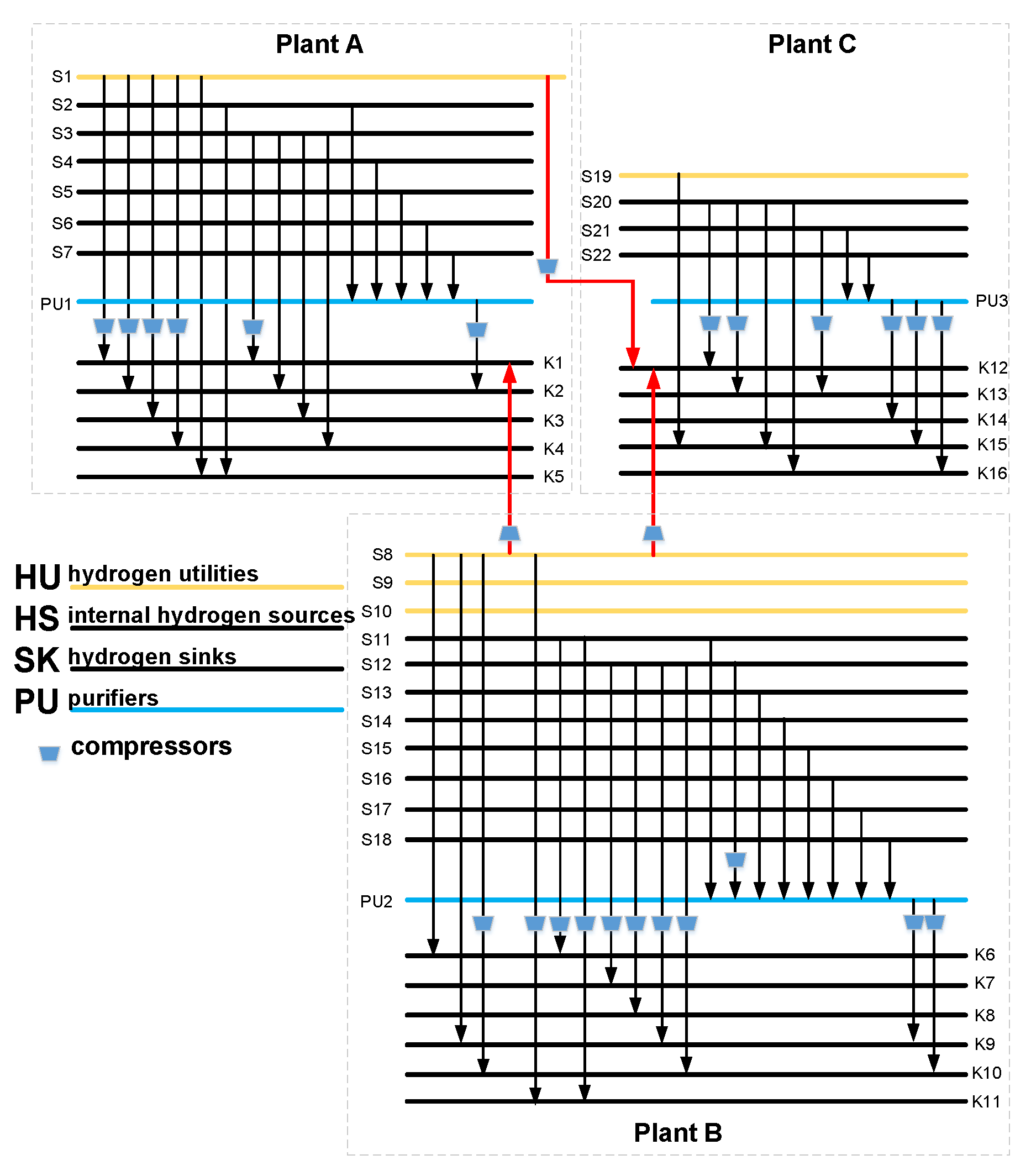
In this case study, there are three plants, denoted by Plant A [17], Plant B [18], and Plant C [5], in a chemical industry park. The distance between Plant A and Plant B is 10 km, and the distance between Plant B and Plant C is also 10 km. Plant A is 20 km away from Plant C.

Hydrogen streams can be delivered among the three plants through cross-plant hydrogen pipelines. The annual operating time of the plants is assumed to be 8000 h. According to Figure 2 and the fluctuating characteristics of hydrogen sources and sinks, the operating time of the inter-plant hydrogen network is divided into seven subperiods, as listed in Table 1, in which the division of the subperiod and the flowrates of each subperiod are also presented. In this case study, the hydrogen utilities include S1, S8, S9, S10, and S19, and their prices are listed in Table 2.

Table 1. Subperiod partitioning of the inter-plant hydrogen network and parameters of hydrogen sources and hydrogen sinks.

Subperiod		1	2	3	4	5	6	7
Plant	S/K	Flowrate [mol·s−1]							H2 Purity [mol%]	Pressure [MPa]
A	S1	1115.0	1115.0	1115.0	1115.0	1115.0	1115.0	1115.0	0.95	2.1
	S2	216.0	216.0	216.0	237.6	237.6	224.7	224.7	0.80	2.1
	S3	113.6	113.6	113.6	126.6	126.6	124.4	124.4	0.80	8.3
	S4	144.8	144.8	144.8	109.5	109.5	180.3	180.3	0.75	2.4
	S5	80.8	80.8	80.8	100.1	100.1	67.9	67.9	0.75	2.8
	S6	20.0	20.0	20.0	14.4	14.4	18.3	18.3	0.70	2.4
	S7	31.2	31.2	31.2	36.5	36.5	25.9	25.9	0.65	1.4
	K1	521.0	521.0	521.0	580.4	580.4	570.3	570.3	0.95	13.8
	K2	486.7	486.7	486.7	367.9	367.9	605.6	605.6	0.93	3.4
	K3	246.7	246.7	246.7	305.8	305.8	207.3	207.3	0.90	4.1
	K4	75.8	75.8	75.8	54.4	54.4	69.5	69.5	0.80	3.4
	K5	54.7	54.7	54.7	64.2	64.2	45.4	45.4	0.75	2.1
B	S8	881.5	881.5	881.5	881.5	881.5	881.5	881.5	0.97	7
	S9	312.1	312.1	312.1	312.1	312.1	312.1	312.1	0.95	1.2
	S10	312.1	312.1	312.1	312.1	312.1	312.1	312.1	0.95	1.2
	S11	124.9	124.9	133.6	133.6	133.6	133.6	131.3	0.90	1.4
	S12	536.9	536.9	509.2	509.2	509.2	509.2	589.3	0.92	1.1
	S13	5.4	5.4	7.1	7.1	7.1	7.1	6.1	0.60	1.4
	S14	20.9	20.9	24.0	24.0	24.0	24.0	16.5	0.46	1.6
	S15	13.2	13.2	10.9	10.9	10.9	10.9	17.3	0.71	1.5
	S16	24.8	24.8	30.9	30.9	30.9	30.9	19.2	0.83	1.5
	S17	90.5	90.5	55.4	55.4	55.4	55.4	81.6	0.76	1.2
	S18	61.2	61.2	52.8	52.8	52.8	52.8	69.3	0.65	1.2
	K6	74.4	74.4	98.6	98.6	98.6	98.6	85.0	0.90	7
	K7	47.4	47.4	54.7	54.7	54.7	54.7	37.5	0.87	5
	K8	156.1	156.1	129.0	129.0	129.0	129.0	203.6	0.92	7
	K9	299.7	299.7	372.8	372.8	372.8	372.8	232.1	0.96	7
	K10	287.2	287.2	175.7	175.7	175.7	175.7	259.0	0.98	10
	K11	549.4	549.4	474.5	474.5	474.5	474.5	622.1	0.94	20
C	S19	496.0	496.0	496.0	496.0	496.0	496.0	496.0	0.999	3.5
	S20	437.1	480.8	480.8	480.8	363.0	363.0	363.0	0.92	3.5
	S21	142.3	103.0	103.0	103.0	137.9	137.9	137.9	0.71	2.5
	S22	21.4	27.0	27.0	27.0	31.4	31.4	31.4	0.70	2.5
	K12	292.6	236.0	236.0	236.0	286.3	286.3	286.3	0.93	13.0
	K13	281.3	332.5	332.5	332.5	373.2	373.2	373.2	0.87	8.7
	K14	28.7	34.8	34.8	34.8	29.6	29.6	29.6	0.87	5.0
	K15	34.1	40.6	40.6	40.6	33.8	33.8	33.8	0.85	3.5
	K16	34.3	29.5	29.5	29.5	26.8	26.8	26.8	0.85	3.0

Table 2. Prices of hydrogen utilities [5,17,18].

Hydrogen Source	S1 [17]	S8 [18]	S9 [18]	S10 [18]	S19 [5]
ehu [CNY·mol−1]	0.01	0.009	0.011	0.011	0.015

In this case, the pressure swing adsorption (PSA) is selected as the centralized purifier. The pressures of PSA for feed stream and product stream are both 1.2 MPa, the hydrogen recovery ratio of PSA is assumed to be 0.9, and the hydrogen purity of the product stream is 99%. The residual stream of PSA is discharged to the fuel gas system, of which the pressure is 0.06 MPa. In the calculation, the fixed cost coefficient a and the variable cost coefficient b for the compressor are 69 and 1.164 [16], and those for the pipeline are 32 and 28.12 [12], and those for the purifier are 302.3 and 14.25 [16]. The electricity price is 0.8 CNY/kW∙h, and the price of heat energy is 0.025 CNY/MJ. In the calculations, the models were coded on GAMS 24.1 platform running on a PC with 2.93 GHz CPU and 6 GB RAM, and CPLEX was used as the solver.

4.2. Optimal Design of Multi-Period Inter-Plant Hydrogen Network

Figure 3 shows the topological structure of the optimal design of the multi-period inter-plant hydrogen network, and the red lines represent the cross-plant pipelines. Results indicate that the centralized purifier is set up for each plant, and the product stream of the purifier only supplies the hydrogen sinks within the same plant. The total number of connections in the hydrogen network is 50, and only three matches across the three plants. Furthermore, it can be seen from Figure 3 and Table 1 that the hydrogen in plant B is relatively surplus in the inter-plant hydrogen network. Since the hydrogen utility S8 in plant B has higher pressure and purity, it is delivered to the hydrogen sinks with high-pressure requirements in Plant A and Plant C through the cross-plant pipelines. In addition, Plant A also supplies hydrogen utility to Plant C.

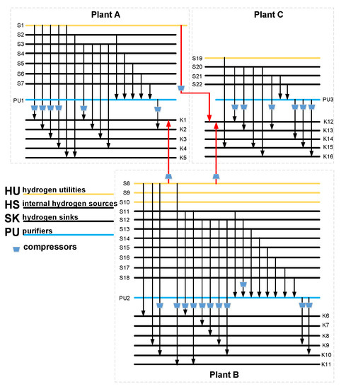
Figure 3. The structure of the inter-plant hydrogen network, obtained by the proposed method.

Table 3 presents the comparison of the effects of integrating the inter-plant hydrogen network with integrating the individual plant hydrogen network. The results show that the utilization of hydrogen is more efficient when the hydrogen streams can be transported among the plants via inter-plant pipelines and compressors, since the consumption of hydrogen utility is reduced by 14.3% compared with the scheme of individual plant integration. The total annual cost decreases by 4.22%. Therefore, the inter-plant integration can effectively achieve the reduction of the operating cost and TAC as well. However, the number of connections increases from 40 to 50, and the investment cost increases by 19.5%, indicating that a more complex network structure is reached.

Table 3. Comparison of the inter-plant integration and individual plant integration.

Item	Inter-Plant Network	Individual Hydrogen Network
	A + B + C	A	B	C	Total
Number of matches	50	15	13	12	40
Consumption of hydrogen in utility [109 mol]	48.424	25.832	24.626	4.872	55.330
Hydrogen cost [108 CNY·y−1]	4.940	2.937	2.234	0.731	5.902
Investment cost [108 CNY·y−1]	0.974	0.377	0.292	0.146	0.815
Operating cost [108 CNY·y−1]	4.429	2.579	1.482	0.756	4.817
TAC [108 CNY·y−1]	5.403	2.956	1.774	0.901	5.631

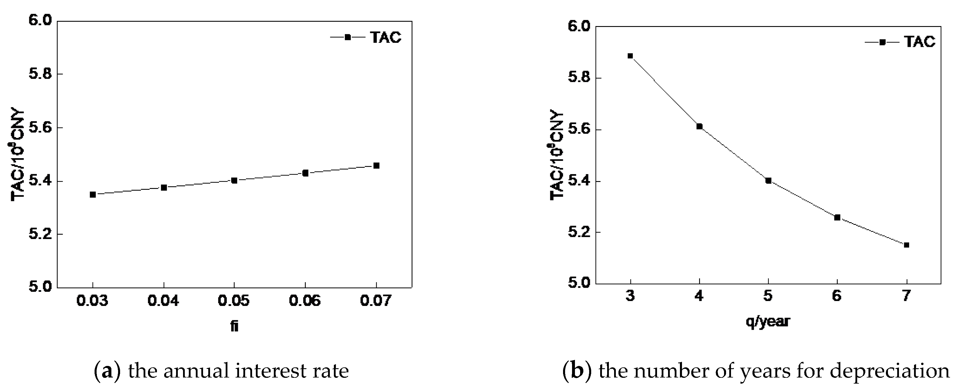
It is also worth mentioning that different values of the annualized factor $Af$ have a big impact on the optimal structure and the scheduling scheme, and according to Equation (2), $Af$ is influenced by the annual interest rate (fi) and the number of years for depreciation (q). Therefore, we analyze the influence of fi and q on $TAC$, as is shown in Figure 4. TAC increases with the growth of the annual interest rate (fi) or the decrease of the years for depreciation (q), and meanwhile, the investment cost of the system is reduced, and the network structure is simplified, but this is at the expense of operation cost.

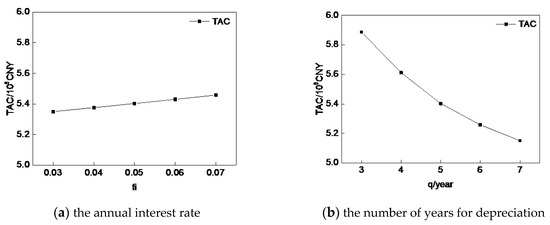
Figure 4. The influence of fi and q on the total annual cost ($TAC$).

4.3. Comparison of the Proposed Method and Other Design Methods

To further clarify the advantages and effectiveness of the proposed method, we compared the simultaneous method and stepwise methods, such as the structure-merged method and the structure-fixed method in this section.

4.3.1. The Results of Structure-Merged Method and Structure-Fixed Method

• The structure-merged method

In this method, the multi-period hydrogen network is synthesized in two steps. In the first step, the single-period optimization model of the inter-plant hydrogen network is solved, and the optimal hydrogen network structure of each subperiod can be obtained. In the second step, the hydrogen network structures of the seven subperiods are merged. The final structure of the inter-plant hydrogen network accommodates all the matches that have ever occurred in all subperiods, and the capacity of pipeline and compressors are assigned to the maximum capacity in all subperiods.

Table 4 shows the number of matches, investment costs, and operation costs of the single period structure and the merged final structure. It can be seen that the investment cost does not increase significantly after the structure merged. The reason is that the structure obtained under each subperiod is similar, and only a few devices are newly constructed. The total matching number of hydrogen networks is 48, which is less than the one obtained by the simultaneous method. However, its investment cost is 16% higher than that of the simultaneous method.

Table 4. Characteristics of the multi-period hydrogen network, obtained by the structure-merged method.

Item	Position	Step1 The Sequence Number of the Optimized Subperiod							Step2 Multi-Period Hydrogen Network
		1	2	3	4	5	6	7
Number of matches	intra- plant	35	35	39	38	36	37	38	45
	inter- plant	2	2	2	2	1	1	2	3
Investment cost [108 CNY·y−1]	intra- plant	0.885	0.864	0.806	0.818	0.844	0.852	0.939	1.056
	inter- plant	0.029	0.029	0.039	0.039	0.035	0.035	0.042	0.071
	total	0.914	0.893	0.845	0.857	0.879	0.887	0.981	1.127
Operation cost [108 CNY·y−1]	total	4.232	4.218	3.981	3.909	4.451	4.793	4.956	4.396

2.

The structure-fixed method

In this method, the first step is to integrate the hydrogen network with the data under the $p^{\mathrm{th}}$ subperiod. The obtained intra-plant structure of the hydrogen network is fixed as the initial structure, whereas the inter-plant structure of the hydrogen network is allowed to extend. Then the optimal design and operation scheme under the other six subperiods are optimized on the basis of the initial structure. It is noted that all of the intra-plant connections newly installed are forbidden. Finally, the obtained structures are merged into the final hydrogen network, and the total annual cost is denoted as $TA{C}_p$. Set $p$ as 1~7 and perform the above steps, respectively. Seven design schemes can be obtained. When the number of subperiod is $p$, the model of the single period hydrogen network is solved $p^2$ times.

Table 5 shows the number of inter-plant and intra-plant matches, investment cost, operating cost, and the TAC of the seven design schemes. It can be seen that compared with the simultaneous method, the number of intra-plant connections decreases, and the number of inter-plant connections increases. The newly added inter-plant pipelines are used to adjust the hydrogen exchange among the plants to meet the hydrogen demand in other subperiods. The selection of the initial structure also affects the structure and cost of the final hydrogen network.

Table 5. Costs and the number of matches for the scheme obtained by the structure-fixed method.

Item	The Sequence Number of the Fixed Subperiod
	1	2	3	4	5	6	7
Number of intra-plant matches	35	35	39	38	36	37	38
Number of inter-plant matches	9	8	5	8	7	4	5
Number of matches	44	43	44	46	43	41	43
Investment cost [108 CNY·y−1]	1.13	1.11	1.10	1.17	1.14	1.06	1.08
Operation cost [108 CNY·y−1]	4.39	4.40	4.39	4.38	4.47	4.47	4.39
Total annual cost [108 CNY·y−1]	5.53	5.50	5.49	5.55	5.61	5.53	5.48

As shown in Table 5, when the structure of the single period hydrogen network scheme obtained under the subperiod 7 is fixed as the initial structure, the total annual cost of the inter-plant hydrogen network is 5.478 × 10⁸ CNY·y⁻¹, which is lower than that of other schemes. This scheme is chosen as the result of the structure-fixed method in the following analysis.

It is worthy of noting that there are seven subperiods in this case. For the structure-merged method and structure-fixed method, we need to solve the model of the single period hydrogen network for 7 times and 49 times, respectively, whereas we simply solved the hydrogen integration model once by using the simultaneous method. Thus, the computation load is reduced.

4.3.2. The Hydrogen Exchange among the Plants

The configuration of cross-plant connections is a significant feature of the inter-plant hydrogen network. In this section, we will discuss the results related to the cross-plant hydrogen matches. According to the abovementioned results, the numbers of the cross-plant matches obtained by the proposed method, the structure-merged method, and the structure-fixed method are 3, 3, and 5, respectively, and the average flowrates of hydrogen exchange in the whole year are 363 mol·s⁻¹, 257 mol·s⁻¹, and 283 mol·s⁻¹, respectively. It appears that, in the proposed method, more hydrogen transportation across the plants is realized by fewer inter-plant connections.

In specific, to reflect the connections among the plants, the amounts of hydrogen exchange via the inter-plant pipelines are listed in Table 6, Table 7 and Table 8. It can be seen from these tables that Plant B always outputs hydrogen to plant A and plant C, and Plant A always exports hydrogen to Plant C. In this case, Plant B supplies surplus hydrogen to the other two plants owing to its utility S8 with higher pressure and lower price, whereas Plant C usually imports hydrogen from other plants because of its own relatively expensive utility.

Table 6. The amount of hydrogen exchange among the plants in the proposed method.

Subperiod		Amount of Pure Hydrogen [mol·s−1]
		A	B	C
1	A			131
	B	189		13
	C
2	A			91
	B	189		13
	C
3	A
	B	189		105
	C
4	A			147
	B	189		105
	C
5	A			147
	B	189		105
	C
6	A			147
	B	126		99
	C
7	A			131
	B	189		13
	C

Table 7. The amount of hydrogen exchange among the plants in the structure-merged method.

Subperiod		Amount of Pure Hydrogen [mol·s−1]
		A	B	C
1	A
	B	80		124
	C
2	A
	B	99		105
	C
3	A
	B	184		105
	C
4	A
	B	184		105
	C
5	A
	B			278
	C
6	A
	B			278
	C
7	A			26
	B			242
	C

Table 8. The amount of hydrogen exchange among the plants in the structure-fixed method.

Subperiod		Amount of Pure Hydrogen [mol·s−1]
		A	B	C
1	A
	B	90		124
	C
2	A
	B	108		106
	C
3	A		19
	B	196		106
	C
4	A		19
	B	196		106
	C
5	A		19
	B	34		269
	C
6	A		19
	B	34		269
	C
7	A			26
	B			242
	C

It is worthy of noting that the cross-plant pipelines are fully used to transport hydrogen among the plants in each subperiod in the scheme obtained by the proposed method, whereas the inter-plant pipelines are idle sometimes in the scheme obtained by the stepwise method, from Plant B to Plant A during the subperiod 5 to the subperiod 7, for example. It implies that in the simultaneous method proposed in this work, the interactions among the subperiods are considered to coordinate the hydrogen demands of each plant. Nevertheless, the interaction among the subperiods is somehow neglected in the stepwise methods.

4.3.3. Economic Analysis of the Three Methods

In this section, we will further discuss the economic performances of the design schemes obtained by the three methods. Table 9 shows the comparison of the costs of design schemes obtained by the stepwise methods and the proposed method. As shown in the table, a more economical design scheme can be obtained by the proposed method. Although the operating cost of the proposed method is slightly higher, the reduction of the investment costs is remarkable.

Table 9. Comparison of costs of design schemes obtained by the three methods.

Method	Cost [108 CNY·y−1]
	Investment				Operation				Total
	Compressor	PSA	Pipeline	Sum	Utility	Electricity	Fuel Profit	Sum
This work	0.581	0.345	0.048	0.974	4.940	1.112	−1.623	4.429	5.403
The structure-merged method	0.688	0.393	0.046	1.127	4.968	1.113	−1.685	4.396	5.523
The structure-fixed method	0.641	0.393	0.050	1.084	4.948	1.120	−1.673	4.395	5.478

It can also be seen from Table 9 that the operating cost accounts for about 80% of the total annual cost, which is composed mostly of the hydrogen utility cost. In the proposed method, the relation among each subperiod is taken into account, leading to a reasonable allocation of hydrogen sources with different pressures and purities. Thus, the utility cost and the electricity expense are both the lowest. Meanwhile, a lower fuel profit is reached by the reduction of fuel gas streams owing to the internal hydrogen sources being directly matched with the sinks.

As shown in Table 9, the investment cost obtained by the proposed method is 0.973 × 10⁸ CNY·y⁻¹, which is 10–14% lower than those obtained by the two stepwise methods. The cost of the compressors and the purifiers are both lower too. The capacities of compressors and purifiers show the same trend, as shown in Table 10.

Table 10. Comparison of the device capacity of the three methods.

Method	Sum of the Compressor Power [kW]	Capacities of PSA Units [mol·s−1]
		A	B	C	Sum
This work	20,051	493	361	130	984
The structure-merged method	23,928	496	465	169	1130
The structure-fixed method	22,372	496	465	169	1130

To further analyze the reduction of investment costs, we will revisit the performances of single period networks listed in Table 4. It indicates that the cost and the equipment capacities of subperiod 7 are the largest among all the subperiods. Since the structure obtained by the stepwise method is based on the structure of the subperiod 7, its investment cost is also larger. In contrast, the design scheme obtained by the simultaneous method is a trade-off among all of the subperiods, and its investment cost is less than the costs for subperiod 7. It can be inferred that the design scheme by using the stepwise methods are a little sensitive to the situation in subperiods. The worst case may be avoided by the simultaneous method, due to considering the interactions among the subperiods.

5. Conclusions

When the hydrogen networks in chemical industry parks are integrated, it is necessary to coordinate the temporal and spatial demand and supply of hydrogen in both the intra-plant and inter-plant. To address the optimization problem of integrating multi-period hydrogen network in multiple plants, a multi-period simultaneous optimization method for the inter-plant hydrogen network integration was proposed, in which the hydrogen supply across the plants is implemented through cross-plant pipelines, and a MILP model is developed for the optimization of inter-plant hydrogen network. A case study of a three-plant hydrogen network with seven subperiods is utilized to demonstrate the effectiveness and advantages of the proposed method. Moreover, the optimal design scheme was compared with those of the stepwise methods, including the structure-merged method and the structure-fixed method.

The results show that the proposed method can give a design and scheduling scheme for the inter-plant hydrogen system with lower TAC. Compared with the stepwise methods, the proposed method simplifies the solving steps and is able to provide a better network structure and scheduling scheme. The investment cost obtained by the proposed method is lower than those obtained by the two stepwise methods. In the proposed method, the interactions among the subperiods are considered to coordinate the fluctuating demand and supply of hydrogen in each plant. The cross-plant pipelines are fully used to transport hydrogen among the plants in each subperiod in the scheme obtained by the proposed method, whereas the inter-plant pipelines are idle sometimes in the scheme obtained by the stepwise methods. The proposed method is suitable for integrating the inter-plant hydrogen system with predictable operational parameters and can also be used to study the influence of inter-plant integration and multi-period operation on the design of the hydrogen system. However, the fluctuations in operating conditions may change randomly in practice. Therefore, the uncertainties should be considered during integration. Of course, it deserves further work in the future.

References

- Hwangbo, S.; Lee, I.-B.; Han, J. Multi-period stochastic mathematical model for the optimal design of integrated utility and hydrogen supply network under uncertainty in raw material prices. Energy 2016, 114, 418–430. [Google Scholar] [CrossRef]
- Jagannath, A.; Elkamel, A.; Karimi, I.A. Improved Synthesis of Hydrogen Networks for Refineries. Ind. Eng. Chem. Res. 2014, 53, 16948–16963. [Google Scholar] [CrossRef]
- Deng, C.; Zhou, Y.; Chen, C.-L.; Feng, X. Systematic approach for targeting interplant hydrogen networks. Energy 2015, 90, 68–88. [Google Scholar] [CrossRef]
- Lou, J.; Liao, Z.; Jiang, B.; Wang, J.; Yang, Y. Robust optimization of hydrogen network. Int. J. Hydrog. Energy 2014, 39, 1210–1219. [Google Scholar] [CrossRef]
- Liang, X.; Kang, L.; Liu, Y. Impacts of Subperiod Partitioning on Optimization of Multiperiod Hydrogen Networks. Ind. Eng. Chem. Res. 2017, 56, 10733–10742. [Google Scholar] [CrossRef]
- Liang, X.; Kang, L.; Liu, Y. The Flexible Design for Optimization and Debottlenecking of Multiperiod Hydrogen Networks. Ind. Eng. Chem. Res. 2016, 55, 2574–2583. [Google Scholar] [CrossRef]
- Kang, L.; Liang, X.; Liu, Y. Design of multiperiod hydrogen network with flexibilities in subperiods and redundancy control. Int. J. Hydrogen Energy 2018, 43, 861–871. [Google Scholar] [CrossRef]
- Kuo, C.-C.; Chang, C.-T. Improved Model Formulations for Multiperiod Hydrogen Network Designs. Ind. Eng. Chem. Res. 2014, 53, 20204–20222. [Google Scholar] [CrossRef]
- Jiao, Y.; Su, H.; Hou, W.; Li, P. Design and Optimization of Flexible Hydrogen Systems in Refineries. Ind. Eng. Chem. Res. 2013, 52, 4113–4131. [Google Scholar] [CrossRef]
- Liu, F.; Zhang, N. Strategy of Purifier Selection and Integration in Hydrogen Networks. Chem. Eng. Res. Design 2004, 82, 1315–1330. [Google Scholar] [CrossRef]
- Deng, C.; Zhou, Y.Y.; Jiang, W.; Feng, X. Optimal design of inter-plant hydrogen network with purification reuse/recycle. Int. J. Hydrogen Energy 2017, 42, 19984–20002. [Google Scholar] [CrossRef]
- Kang, L.; Liang, X.; Liu, Y. Optimal design of inter-plant hydrogen networks with intermediate headers of purity and pressure. Int. J. Hydrogen Energy 2018, 43, 16638–16651. [Google Scholar] [CrossRef]
- Lou, Y.; Liao, Z.; Sun, J.; Jiang, B.; Wang, J.; Yang, Y. A novel two-step method to design inter-plant hydrogen network. Int. J. Hydrogen Energy 2019, 44, 5686–5695. [Google Scholar] [CrossRef]
- Shehata, W.M.; Shoaib, A.M.; Gad, F.K. Inter-plant hydrogen integration with regeneration placement and multi-period consideration. Egypt. J. Pet. 2018, 27, 553–565. [Google Scholar] [CrossRef]
- Wu, S.; Liu, G.; Yu, Z.; Feng, X.; Liu, Y.; Deng, C. Optimization of hydrogen networks with constraints on hydrogen concentration and pure hydrogen load considered. Chem. Eng. Res. Des. 2012, 90, 1208–1220. [Google Scholar] [CrossRef]
- Hallale, N.; Liu, F. Refinery hydrogen management for clean fuels production. Adv. Environ. Res. 2001, 6, 81–98. [Google Scholar] [CrossRef]
- Elkamel, A.; Alhajri, I.; Almansoori, A.; Saif, Y. Integration of hydrogen management in refinery planning with rigorous process models and product quality specifications. Int. J. Process Syst. Eng. 2011, 1, 302–330. [Google Scholar] [CrossRef]
- Liao, Z.; Wang, J.; Yang, Y.; Rong, G. Integrating purifiers in refinery hydrogen networks: A retrofit case study. J. Clean. Prod. 2010, 18, 233–241. [Google Scholar] [CrossRef]
Publisher’s Note: MDPI stays neutral with regard to jurisdictional claims in published maps and institutional affiliations. |
© 2020 by the authors. Licensee MDPI, Basel, Switzerland. This article is an open access article distributed under the terms and conditions of the Creative Commons Attribution (CC BY) license (http://creativecommons.org/licenses/by/4.0/).