Numerical Simulation and Experimental Research on Flow Force and Pressure Stability in a Nozzle-Flapper Servo Valve

Abstract

In the nozzle flapper servo valve, the transient flow force on the flapper is the fundamental reason that affects the pressure stability. The pressure pulsation in the pilot stage causes forced vibration of the flapper, and its deviation will directly influence the control pressure difference, which will make the pressure appear unstable. In order to grasp the principle and characteristics of transient flow force and its influence on pressure stability, a mathematical model of flapper displacement and control pressure is derived. For collecting the dynamic changes of the transient flow force and recording the motion behavior of the flapper, a three-dimensional model of the pilot-stage is established. Numerical simulations of turbulence phenomenon analysis are conducted with a variation of flapper displacement ranging from 5 $\mathsf{\mu }$m to 20 $\mathsf{\mu }$m. It can be concluded that the change trend of the flapper displacement is similar to the steady-state flow force and the transient flow force pulsation amplitude. Under the same structural parameters, the pulsating frequency of the flow force remains basically constant. The fluctuation of the flow force of the pilot stage will cause the pressure of the servo valve control cavity to vibrate to a certain extent, which is a factor that cannot be ignored that affects the output stability of the servo valve.

1. Introduction

As a control element in the electro-hydraulic servo system, the servo valve converts the input low-power electric signal into high-power hydraulic energy output, which plays an important role in many fields such as aerospace. Nozzle flapper servo valves are widely used in hydraulic servo systems due to their advantages of fast dynamic response, high control accuracy, and compact structure. At the earliest, Merritt [1] proposed a third-order mathematical model of the servo valve which caused high accuracy and was widely used. In the future research, some nonlinear effects are considered, and the performance of the servo valve is described more accurately through high-order mathematical models. Kim [2] believes that spool resonance and pressure feedback on the spool are more important, and, based on this, a five-order system model of the servo valve is established. Based on the theory of differential geometry, Mu [3] considers the high-order nonlinear terms in the system, and applies the input and output linearization method to the mathematical modeling of the servo valve. On this basis, considering the two degrees of freedom of the armature-flapper assembly, a seventh-order model of the dynamic response of the electro-hydraulic servo valve is derived from the nonlinear equation [4].

In view of the problem that the traditional servo valve modeling method cannot describe the servo valve system from the component level, the object-oriented Modelica modeling language is used to model the entire valve [5]. Considering the nonlinear terms that are often limited in establishing the description equations, Dasgupta and Murrenhoff [6] used a Bond diagram technique to establish a comprehensive dynamic model of the hydraulic motor drive system.Using the bond graph method has the advantage of dealing with complex systems with multiple energy domains. The servo valve can be modeled according to its electromechanical coupling characteristics [7]. Although researchers have added more nonlinear parts in the servo valve modeling process, it is still difficult to accurately express the parts with complex flow fields. The pilot stage is a key part of driving the movement of the spool, and the position of the flapper will directly affect the stability of the servo valve output. Hayashi [8] uses Navier–Stokes equations and continuity equations to describe the flow in the flat-faced nozzle-flapper valve. With the development of numerical simulation technology, scholars have continuously deepened the research on the flow force of the flapper. Mchenya [9] studied the flow field distribution in the pilot-stage of the servo valve and the relationship between the flow rate and the pressure drop across the nozzle. Under different inlet velocities and different geometric model sizes, Li [10] simulated the flow field distribution, vortex and pressure oscillation changes in the jet flow field. Subsequently, Li [11] conducted experimental observations within the range of Reynolds number from 630 to 2500, and compared it with the CFD simulation results to confirm the occurrence and location of the cavitation source.

Based on Li’s research, Aung [12] conducted a numerical study on the cavitation phenomenon of the pilot stages of different flapper shapes in order to find a reasonable flapper shape to reduce cavitation. In order to gain insight into the phenomena caused by high-frequency noise and servo valve vibration, Zhang [13] used Large Eddy Simulation (LES) coupled with a cavitation model to simulate the unstable cavitation shedding around the sharp edges of the flapper. Li [14] performed numerical simulations on the flow coefficient for different gap widths and inlet pressures, and the flow coefficient mainly went through three stages: the linear throttling section, transition section, and saturation section. Yang [15] proposed to replace the traditional round nozzle with a diamond nozzle to reduce cavitation in the flow. The research on the internal flow force of the servo valve has always been a problem that plagues researchers. Initially, researchers tried to use momentum theory to estimate the fluid force acting on the flapper and expressed it as a function of nozzle pressure and nozzle-flapper gap [16]. With the development of numerical simulation technology, due to the complexity and uncertainty of the flow field, it is difficult to accurately describe the transient changes of the flow field only by deriving theoretical formulas [17].

Since the position, shape, and flow angle move with the movement of the component, the CFD method can predict the flow force more accurately than the traditional theoretical method [18]. The slide valve is a mechanism that directly controls the output, and the study of its flow force has attracted more scholars’ attention [19,20]. The influence of flow force on the spool balance of hydraulic components is well known, and it covers the expression from analysis to experimental evaluation to CFD analysis. By accepting a further approximation to the compressibility of the fluid, the transient flow can be further expanded. As the key component of the pilot stage to control the movement of the spool valve, its transient characteristics are beginning to attract attention [21]. The transient flow field distribution and the periodic characteristics of the flapper resonance motion may be affected by the internal fluid–structure interaction of the pilot stage [22]. Subsequently, in order to grasp the force and characteristics of the armature assembly and the source of the excited vibration, the fluid forces with different inlet pressure and deflection were analyzed [23]. The CFD numerical simulation technology is widely used in the difficult-to-observe area inside the container, and the impact is analyzed according to the fluid flow characteristics [24,25].

The periodic characteristics of the transient flow field will cause the flapper to vibrate, which may cause pressure pulsation in the pilot stage cavity while generating noise. This paper derives the mathematical model between the pilot stage and the spool valve control pressure difference, and uses transient numerical simulation to analyze the pressure pulsation and hydrodynamic oscillation trend of the pilot stage flow field. Based on the numerical simulation data fitting of the flow force when different flapper displacements, the influence of the flow force in the pilot stage on the pressure stability of the control chamber is studied. Through the comparative analysis of experiment and simulation, the mathematical model and simulation results are verified.

2. Working Principle of the Nozzle Flapper Servo Valve

As shown in Figure 1, the nozzle flapper pressure servo valve is composed of torque motor, armature assembly, pilot-stage, and spool valve. The torque motor acts as the driving part of the servo valve, which is composed of a magnetic conductor, permanent magnet, and control coil. Permanent magnets and permeable magnets form a closed magnetic circuit, which generates inherent magnetic flux in the circuit. When the coils at both ends of the armature input the control current, the control magnetic flux is generated in the magnetic circuit composed of the armature and the permeable magnet. Due to the difference in the direction of the control magnetic flux and the fixed magnetic flux in the air gap, electromagnetic force is generated on the armature. The electromagnetic force drives the armature to rotate around the top of the spring tube, and the connecting rod drives the flapper to deflect.

The pilot stage assembly is mainly composed of flapper and nozzles, which are similar in principle to variable orifices. When the high-pressure oil passes through the oil filter and the fixed orifice, it enters the transfer chamber. The chamber is respectively connected with the nozzle chamber of the pilot stage and the control chamber at both ends of the spool. When the flapper deflects, the flow rate of the variable orifice changes, which in turn affects the flow rate into the control chambers on both sides of the spool valve, and realizes the control of the control pressure difference. The pressure difference pushes the spool valve to move, realizing the switch between the oil supply port, the oil return port, and the output port. The two ends of the spool valve are designed with feedback chambers that are connected to the output chamber and the oil return chamber, respectively. When the control force and feedback force are in equilibrium, the spool valve is stable in the neutral position (input, output, and return ports are not connected to each other), and the servo valve outputs a current proportional to the input current.

3. Kinematics Mathematical Model

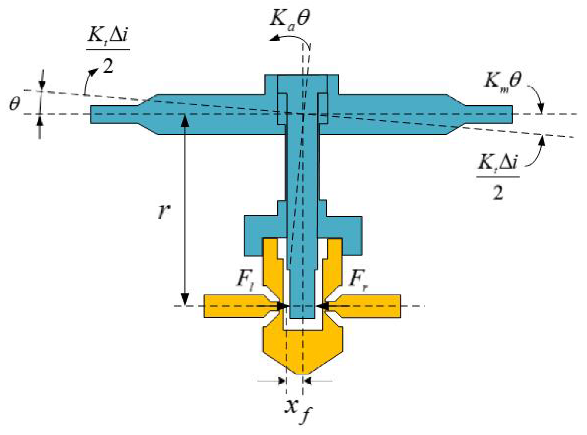
As shown in Figure 2, the armature assembly is mainly composed of armature, spring tube, transmission rod, and flapper. The armature assembly acts as a bridge in the pilot stage, transmitting the rotation of the armature to the flapper. The armature is subjected to the electromagnetic torque generated by the torque motor. Under the combined action of the electromagnetic torque and the recovery torque of the spring tube, the mechanical movement of the flapper in angular form is realized. Under the joint action of the moment $K_m\theta$ generated by the fixed magnetic flux and the moment $K_t\mathsf{\Delta }i/2$ generated by the control magnetic flux, the armature produces a deflection motion.

During the rotation of the armature, due to the balance of the bending moment of the spring tube, the hydrodynamic torque and the electromagnetic moment of the flapper, the equation of motion of the armature assembly is

$$T_d=(J_a{s}^2+B_{a}s+K_a)\theta +F_{flow}r$$

(1)

where $T_d$ is the electromagnetic moment, $J_a$ is the rotational inertia of the armature assembly, $B_a$ is the viscous damping coefficient of the armature assembly, $K_a$ is the spring tube stiffness, and $F_{flow}$ is the flow force received on the flapper, and r is the radius of rotation. In the pilot-stage, the position of the flapper is not stable due to the influence of the pulsating flow force. Considering the changing state of the flapper position, the purpose is to obtain the mathematical expression of the flow force on the flapper. Therefore, the control body shown in Figure 3 is selected. The momentum equation is established in the x-axis direction to calculate the flow force on the flapper.

The outflow of nozzle can be given by the orifice equation

$$Q_{n1}=\pi C_{dn}{D}_N\left(x_{f0}+x_f\right)\sqrt{\frac{2\left(p_1-p_0\right)}{\rho }}$$

(2)

$$Q_{n2}=\pi C_{dn}{D}_N\left(x_{f0}-x_f\right)\sqrt{\frac{2\left(p_2-p_0\right)}{\rho }}$$

(3)

where $Q_{n1}$ and $Q_{n2}$ are the flow out of the nozzles on both sides, respectively, $C_{dn}$ is the flow coefficient at the nozzle, $D_N$ is the diameter of the nozzle, $x_{f0}$ is the initial gap between the flapper and the nozzle, and $x_f$ is the displacement of the flapper, $p_1$ is the pressure of the nozzle cavity, $p_0$ is the return pressure, and $\rho$ is the density of the oil.

The pressure at the nozzle is given by the Bernoulli equation

$$p_{o1}=p_1+\frac{1}{2}\rho v_1^2$$

(4)

$$p_{o2}=p_2+\frac{1}{2}\rho v_2^2$$

(5)

where $p_{o1}$ and $p_{o2}$ are the total pressure at the nozzle, and $v_1$ and $v_2$ are the velocity at the nozzle.

The flow velocity at the nozzle can be expressed as

$$v_1=\frac{4Q_{n1}}{\pi D_N^2}$$

(6)

$$v_2=\frac{4Q_{n2}}{\pi D_N^2}$$

(7)

The momentum equation in the x-direction can be expressed as

$$\frac{\pi D_N^2}{4}{p}_1-F_l=\rho Q_{n1}\frac{d{x}_f}{dt}+\rho Q_{n3}\frac{d{x}_f}{dt}-\rho Q_{n1}{v}_1$$

(8)

where $F_l$ is the flow force on the left side of the flapper.

The flow that pushes the flapper to move can be expressed as

$$Q_{n3}=Q_{n1}-\frac{\pi D_N^2}{4}\frac{d{x}_f}{dt}$$

(9)

Therefore, the flow force on the flapper can be expressed as

$$F_l=\frac{\pi D_N^2}{4}\left[p_1+\rho {\left(v_1-\frac{d{x}_f}{dt}\right)}^2\right]$$

(10)

$$F_r=\frac{\pi D_N^2}{4}\left[p_2+\rho {\left(v_2+\frac{d{x}_f}{dt}\right)}^2\right]$$

(11)

The combined flow force on the flapper can be expressed as

$$F_{flow}=F_l-F_r=\frac{\pi D_N^2}{4}\left(p_1-p_2\right)+\rho \left(Q_{n1}+Q_{n2}\right)\left(\frac{Q_{n1}-Q_{n2}}{A_N}-2\frac{d{x}_f}{dt}\right)$$

(12)

It can be concluded from the simulation results of the pilot-stage flow field that the pressure on the flapper is not linearly distributed. Based on the momentum theorem of hydrodynamics, the steady-state flow force can be expressed as

$$F_{fm}=A_N{K}_p{x}_f+4\pi C_{df}^2\left[K_p{x}_f^3-2\left(K_{p1}+K_{p2}\right)x_f^2{x}_{f0}+K_p{x}_f{x}_{f0}^2\right]$$

(13)

At the same time, the unstable transient flow force generated by the flow can be expressed as

$$F_{fs}=2\rho \left(Q_{n1}+Q_{n2}\right)\frac{d{x}_f}{dt}$$

(14)

As shown in Figure 4, when the high-pressure fluid passes through the fixed orifice, the flow into the nozzle cavity can be expressed as

$$Q_{mn1}=C_{dp}{A}_p\sqrt{\frac{2\left(p_{m1}-p_1\right)}{\rho }}$$

(15)

$$Q_{mn2}=C_{dp}{A}_p\sqrt{\frac{2\left(p_{m2}-p_2\right)}{\rho }}$$

(16)

where $C_{dp}$ is the flow coefficient of the flow path between the transition cavity and the nozzle cavity, $A_p$ is the cross-sectional area of the flow channel, and $p_{m1}$ and $p_{m2}$ are the pressure of the transition cavity on both sides.

Based on the continuity equation, the relationship between the flow into the nozzle chamber and the flow out of the nozzle can be obtained:

$$Q_{mn1}=Q_{n1}$$

(17)

$$Q_{mn2}=Q_{n2}$$

(18)

According to Formulas (2), (3), and (15)–(18), the pressure in the transfer cavity after passing through the fixed orifice can be obtained:

$$p_{m1}=\frac{{\pi }^2{C}_{dn}^2{D}_N^2{(x_{f0}+x_f)}^2}{C_{dp}^2{A}_p^2}\left(p_1-p_0\right)+p_1$$

(19)

$$p_{m2}=\frac{{\pi }^2{C}_{dn}^2{D}_N^2{(x_{f0}-x_f)}^2}{C_{dp}^2{A}_p^2}\left(p_2-p_0\right)+p_2$$

(20)

When the flapper moves, the pressure in the control chamber at both ends of the spool will change. Under the effect of the pressure difference in the control chamber, the spool is pushed to produce a horizontal movement. The sum of the flow into the nozzle chamber and the control chamber can be expressed as

$$Q_l=C_{ds}{A}_s\sqrt{\frac{2\left(p_h-p_{m1}\right)}{\rho }}$$

(21)

$$Q_r=C_{ds}{A}_s\sqrt{\frac{2\left(p_h-p_{m2}\right)}{\rho }}$$

(22)

where $C_{ds}$ is the flow coefficient of fixed orifice, $A_s$ is the cross-sectional area of the fixed orifice, and $p_h$ is the pressure of the oil source.

The flow into the control cavity can be expressed as

$$Q_{mv1}=Q_l-Q_{mn1}=C_{ds}{A}_s\sqrt{\frac{2\left(p_h-p_{m1}\right)}{\rho }}-C_{dp}{A}_p\sqrt{\frac{2\left(p_{m1}-p_1\right)}{\rho }}$$

(23)

$$Q_{mv2}=Q_r-Q_{mn2}=C_{ds}{A}_s\sqrt{\frac{2\left(p_h-p_{m2}\right)}{\rho }}-C_{dp}{A}_p\sqrt{\frac{2\left(p_{m2}-p_2\right)}{\rho }}$$

(24)

The flow into the control cavity can also be written as

$$Q_{mv1}=C_{dv}{A}_p\sqrt{\frac{2\left(p_{m1}-p_{v1}\right)}{\rho }}$$

(25)

$$Q_{mv2}=C_{dv}{A}_p\sqrt{\frac{2\left(p_{m2}-p_{v2}\right)}{\rho }}$$

(26)

Taking into account the compressibility of the oil and the change of the spool valve position, the pressure in the control chamber can be expressed as

$$\frac{d{p}_{v1}}{dt}=\frac{\epsilon }{V_0+A_v{x}_v}\left(Q_l-Q_{mn1}+A_v{v}_v\right)$$

(27)

$$\frac{d{p}_{v2}}{dt}=\frac{\epsilon }{V_0-A_v{x}_v}\left(Q_r-Q_{mn2}-A_v{v}_v\right)$$

(28)

where $V_0$ is the initial volume of the control cavity, $A_v$ is the annular area of the control end face at both ends of the spool, $x_v$ is the displacement of the spool, and $v_v$ is the movement speed of the spool.

The spool moves under the combined action of the pressure difference in the control chamber, the pressure difference in the feedback chamber, and the return spring. With the deviation of the flapper, a control pressure difference will be generated in the control chamber on both sides of the spool. The feedback chamber is connected to the oil return chamber and the output chamber through the flow passage in the valve inner chamber. The dynamic equation of the spool is expressed as

$$\begin{array}{c}\hfill \left(p_{v1}-p_{v2}\right)A_v-(p_s-p_r)A_f=m_v{\ddot{x}}_v+B_v{\dot{x}}_v+K_{flow}{x}_v+K_h{x}_v\end{array}$$

(29)

where $\mathsf{\Delta }{p}_v$ is the pressure difference in the control chamber, $p_r$ is the pressure in the return chamber, $p_s$ is the output pressure, $A_v$ is the annular area of the control chamber, and $A_f$ is the annular area of the feedback chamber. $m_v$ is the mass of the spool, $x_v$ is the displacement of the spool, $K_{flow}$ is the flow force stiffness, and $K_h$ is the stiffness of the return spring.

4. Numerical Simulation

The three-dimensional numerical simulation model of pilot-stage is established in solidworks, and the accurate calculation domain is extracted in geometry as shown in Figure 5. In the modeling process, the displacement of the flapper was considered to range from 0 $\mathsf{\mu }$m to 20 $\mathsf{\mu }$m, and the pressure characteristics of the flow field at different offset positions of the flapper were analyzed. In addition, the 21 MPa high-pressure oil enters the valve through the pressure inlet, and then enters the orifice of the oil filter. The oil in the orifice has a certain pressure loss. The oil enters the left and right chambers of the oil filter through the orifice. The oil filter chamber is divided into two branches, which are respectively connected to the nozzle and the spool control chamber. The established flow field model includes all the flow fields from the high-pressure oil inlet to the pilot-stage, and finally into both ends of the spool.

The density fluid of the hydraulic oil is 850 kg/m${}^3$, the dynamic viscosity is 0.0085 Pa·s. In the grid generation system, a locally encrypted grid is provided, which aims to focus on small parts and reduce the calculation time, effectively improving the calculation accuracy in the pilot-stage chamber. The combination of tetrahedral and hexahedral elements is used to cut geometric shapes due to their flexibility. Unstructured grids are convenient for controlling grid size and node density, and are more suitable for flow field analysis of complex structures. In order to improve the calculation speed and the accuracy of the simulation results, the pilot-stage flow field meshing model uses a structured tetrahedral mesh. A boundary layer grid is set at the contact layer between the fluid and the inner wall of the pipeline, and the grid of the detail part is locally refined to detect that the grid has no negative volume. Three-dimensional fluid calculation domain models with different offset positions of the flapper are imported into FLUENT for calculation. The boundary conditions of the computational domain are shown in Figure 6. The pressure inlets inlet_left and inlet_right on both sides of the pilot stage are pressure inlets, the pressure outlet at the bottom, and the remaining boundary has no sliding wall surface. Areas with large flow velocity or pressure gradient are locally encryption. The surfaces that need to collect steady-state and transient flow force data are wall_left and wall_right.

When the ordered axisymmetric disturbance in the shear layer collides with the flapper, a pressure pulsation of a certain frequency is generated. The pressure pulse is reflected upstream at the speed of sound and passed to the initial separation zone of the shear layer that is sensitive to disturbances, where vorticity pulsation is generated. The turbulent flow field is mainly characterized by randomness, vorticity, and dissipation. The characteristic quantities of each fluid change with time and the spatial displacement presents special pulsations. The natural vibration of external machinery caused by fluid-induced vibration is an unsteady fluid-solid coupling dynamics problem. It is difficult to use a single and deterministic mathematical analysis method to solve the turbulence equation.

In order to better simulate the turbulent flow, the Large Eddy Simulation (LES) method is used to simulate the transient flow field motion. In the large-scale eddy simulation, the large-scale three-dimensional turbulent motion is directly calculated by the instantaneous Navier–Stokes equation, while the influence of the small-scale vortex on the large-scale vortex is reflected in the instantaneous Navier–Stokes equation for the large-scale vortex through a certain model come out. By using the filter function, each variable is divided into two parts: the large-scale average component and the non-scale component.

The Navier–Stokes equation and the continuous equation in the instantaneous state after processing by the filter function are written as

$$\begin{array}{c}\hfill \frac{\partial }{\partial t}\left(\rho {\overline{u}}_i\right)+\frac{\partial }{\partial x_j}\left(\rho {\overline{u}}_i{\overline{u}}_j\right)=-\frac{\partial \overline{p}}{\partial x_i}+\frac{\partial }{\partial x_j}\left(\mu \frac{\partial {\overline{u}}_i}{\partial x_j}\right)-\frac{\partial {\tau }_{ij}}{\partial x_j}\end{array}$$

(30)

$$\frac{\partial \rho }{\partial t}+\frac{\partial }{\partial x_i}\left(\rho {\overline{u}}_i\right)=0$$

(31)

where ${\overline{u}}_i$ and ${\overline{u}}_j$ are the field variables after rate filtering, and the sub-grid scale stress ${\tau }_{ij}=\rho \overline{u_i{u}_j}-\rho \overline{u_i}\overline{u_j}$ is used to reflect the influence of the motion of the small-scale vortex on the solved equation of motion. According to the Smagorinsky basic SGS model, the SGS stress should have the following form:

$${\tau }_{ij}-\frac{1}{3}{\tau }_{kk}{\delta }_{ij}=-2{\mu }_t{\overline{S}}_{ij}$$

(32)

where ${\mu }_t$ is the turbulent viscosity at the sub-grid scale.

$${\mu }_t={\left(C_s\mathsf{\Delta }\right)}^2\left|\overline{S}\right|$$

(33)

$${\overline{S}}_{ij}=\frac{1}{2}\left(\frac{\partial {\overline{u}}_i}{\partial x_j}+\frac{\partial {\overline{u}}_j}{\partial x_i}\right)$$

(34)

$$\left|\overline{S}\right|=\sqrt{2{\overline{S}}_{ij}{\overline{S}}_{ij}}$$

(35)

$$\mathsf{\Delta }={\left({\mathsf{\Delta }}_x{\mathsf{\Delta }}_y{\mathsf{\Delta }}_z\right)}^{1/\phantom{13}3}$$

(36)

where ${\mathsf{\Delta }}_i$ is the grid size along the i axis and $C_s$ is the Smagorinsky constant.

When solving the N-S equation, the SIMPLEC method is used to solve the pressure–velocity coupling. The SIMPLEC method is developed from the SIMPLE method, and the pressure–velocity relationship obtained through the continuity equation and the momentum equation is iterated continuously until it reaches mass conservation. On this basis, the velocity and pressure fields are solved. The SIMPLEC method can still have a good quality conservation effect under the condition of large mesh distortion, and the sub-relaxation iteration can accelerate the convergence speed. The pressure term discretization uses the PRESTO! format, which is suitable for tetrahedral and hexahedral mesh elements. In addition, it can achieve higher accuracy in the calculation of high vortex flow and multiphase flow. Momentum terms are discretized using a second-order upwind style. This format can effectively prevent the dissipation of small-scale vortices in the calculation process. The continuity equation, momentum equation, and turbulence equation are used in the calculation process.

The pressure–velocity relationship obtained through the continuity equation and the momentum equation iterates continuously until the conservation of mass is reached, and then the velocity field and the pressure field are solved.The gradient term uses the Green–Gauss element method, and the pressure term is discrete using the PRESTO! format, which is suitable for tetrahedral and hexahedral grid elements, and can achieve high accuracy in the calculation of high vortex flow and multiphase flow. The discretization of the momentum term uses the second-order upwind style, which can effectively prevent the dissipation of small-scale vortices in the calculation process; the second-order upwind style is used for the gas volume fraction term. At the same time because the LES method is a direct numerical simulation to a certain extent, the second-order precision format is selected for the time term discrete. Since the oil return orifice is added to the servo valve structure, it effectively reduces the generation of cavitation in the pilot stage. Therefore, in the numerical simulation process, the common effect of air and liquid two phases is not considered, and only the influence of vortex on transient flow force is analyzed.

5. Experimental Setup

The pressure characteristics of the control chamber of the nozzle flapper servo valve calculated by the combination of theoretical formula and numerical simulation are verified by the experiment. The pressure stability of the control chamber is an important index related to the output characteristics of the entire valve. Therefore, in order to verify the accuracy of the mathematical model and the numerical calculation results of CFD, the pressure data of the control cavity will be collected experimentally for comparison.

The experimental device mainly includes pump, pipeline, relief valve, pressure sensor, nozzle flapper servo valve, pressure gauge, and signal acquisition equipment, as shown in Figure 7. The 21 MPa pressure hydraulic oil of the rated hydraulic pump is supplied by the hydraulic pump. Pressure gauges with a measuring range of 0–16 MPa are placed on the oil supply, oil return, and output pipelines. Pressure sensors are set at both ends of the spool in the control cavity, and signal acquisition equipment is used to record pressure data. The pressure sensor of model FYB26 is adopted, and the range is 0–35 MPa, and the accuracy is ±2%. The nozzle flapper pressure servo valve used in the experiment is newly designed to better meet the requirements of high reliability and small size.

6. Results and Discussion

When the flapper moves to a certain position, the main flow force on the flapper also becomes relatively stable. The high-speed oil sprayed from the nozzle is blocked by the flapper, the kinetic energy is converted into pressure energy, and pressure recovery is generated on the flapper. Therefore, there is a local high-pressure circular area near the center of the flapper, and a negative pressure ring will also appear near the center of the nozzle. The acting area of the hydrodynamic force on the flapper is not accurate, and the pressure distribution on the flapper plane should be considered. Collect evenly distributed point cloud data on the surface of the flapper, and draw pressure clouds on the flapper on both sides at different deflection displacements. The pilot-stage three-dimensional symmetrical contour size and pressure clouds of different offsets are shown in Figure 8. Under the same inlet pressure conditions, stable peak areas are formed intensively, and the area of the nozzle projected on the flapper is approximately the same as the size of the high-pressure area. The a, b, c respectively represent the pressure on the flapper surface when the flapper displacement is 15 $\mathsf{\mu }$m, 25 $\mathsf{\mu }$m and 35 $\mathsf{\mu }$m. The left and right columns are the pressure distribution on the left and right sides of the flapper.

Collect the flow force data on both sides of the flapper through FLUENT to obtain the simulation data. Through steady-state flow field analysis, the pressure of each grid cell is obtained. Sum the product of pressure and grid area to get the expression of the flow force on the flapper can be expressed as

$$F_{flow}=\sum _{i=1}^m{A}_i{P}_i-\sum _{j=1}^m{A}_j{P}_j$$

(37)

In previous studies, to facilitate the establishment of models, the flow force was simplified to a certain extent. The pressure that generates the flow force includes: the first part is the pressure on the nozzle area, the second part is the linear gradient pressure between the nozzle pressure and the return pressure on the flapper, and the third part is the return pressure.The linearized form of the flow force on one side of the flapper is

$$F_l=p_1\frac{\pi }{4}{D}_N^2+p_0\frac{\pi }{4}\left(D_f^2-D_N^2\right)$$

(38)

where $D_f$ is the diameter of the baffle, $D_N$ is the inner diameter of the nozzle, $p_1$ is the nozzle pressure, and $p_0$ is the oil return pressure.

The function fitting of the flow force difference data can be obtained as the deviation of the flapper increases, and the curve of numerical simulation and theoretical calculation of flow forces on the two sides of the flapper is shown in Figure 9.

The equation of the fitting curve of the flow force can be expressed as

$$F_{fm}=a{x}_f^3+b{x}_f^2+c{x}_f$$

(39)

where $a=1.1\times {10}^{14}\mathrm{N}/{\mathrm{m}}^3$, $b=3\times {10}^9\mathrm{N}/{\mathrm{m}}^2$, $c=5.7\times {10}^4\mathrm{N}/\mathrm{m}$.

When the deviation of the flapper increases, the pressure difference data of the control cavity can be obtained for function fitting. Numerical simulation and fitting curve of pressure in nozzle cavities are shown in Figure 10.

Based on the numerical analysis of the flow field inside the pilot stage, the pressure data of the nozzle cavity corresponding to different flapper displacements are obtained, as shown in Figure 10. The fitting relationship between flapper displacement and nozzle cavity pressure difference is expressed as

$$\mathsf{\Delta }P=84.43x_f$$

(40)

In order to observe the change of turbulence in the pilot stage, the longitudinal section at the center of the nozzle is selected. Figure 11 shows the turbulence distribution at the profile in a period. In the pilot stage shown in the figure, the flappers are all deflected to the left, and the radial clearance on the right is reduced. Since the pilot stage has a symmetrical structure at the zero position, it is only necessary to consider the situation where the flapper deflects to one side. There is a large-scale vortex on the both sides of the flapper in the area above the nozzle, and the vortex does not show a large change with time. In the area under the nozzle, there is only a large-scale vortex on the larger radial gap of the flapper, and the vortex exhibits regular contraction and expansion in one cycle.

The two sides of the flapper are selected as the detection object, and the flow force on the moving direction of the flapper is calculated. The flow force is a random signal, and theoretically it should contain extensive frequency domain information. The choice of numerical simulation strategy should grasp the main aspects of the problem without losing key information. In order to capture the details of the morphological evolution of the transient vortex in the flow field, based on the characteristic scale and characteristic velocity of the flow field, the time step for transient calculation in this paper is 0.0001 s. Choosing a relatively large time step can not only obtain relatively accurate changes in transient variables, but also reflect the trend of changes in the main components during the transient process.

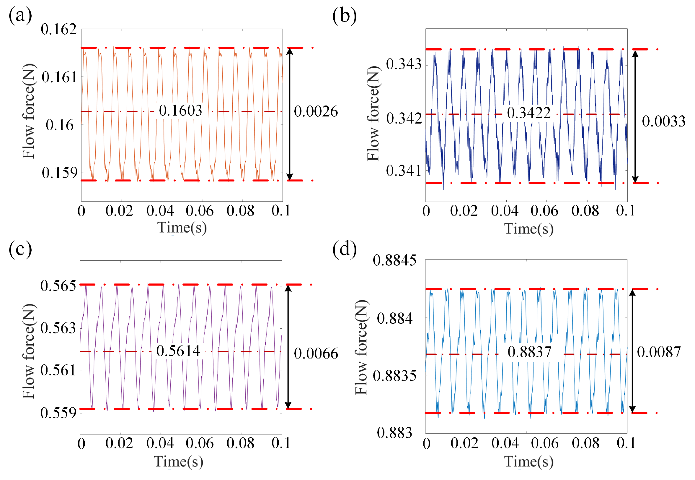
Numerical simulation results of transient flow force on a flapper are shown in Figure 12a,d correspond to 5 $\mathsf{\mu }$m∼20 $\mathsf{\mu }$m, respectively. The central value corresponds to the steady state flow force, and the transient flow force fluctuates around the steady state value. It can be found that, as the offset of the flapper enhances, the amplitude of the transient flow force vibration raises, and the increasing trend is linear. In order to analyze the frequency of the pulsation more intuitively, the fast Fourier transform is performed on the result of the flow force pulsation, and the result of converting the time domain data into frequency domain information is shown in Figure 13.

Therefore, the expression of transient flow dynamics at different flapper displacements is obtained through data fitting

$$F_{fs}=428x_{f}sin(2\pi \times 130)$$

(41)

During the position change of the flapper, all the flow forces received are the sum of steady and transient flow forces. Therefore, the total flow force can be expressed as

$$F_{flow}=F_{fm}+F_{fs}=1.1\times {10}^{14}{x}_f^3-3\times {10}^9{x}_f^2+5.7\times {10}^4{x}_f+428x_{f}sin(2\pi \times 130)$$

(42)

The whole valve transfer function model is established by using the mathematical model in this paper. Given the control current of 40 mA, the step response curve of the whole valve is obtained, and the pressure data of the control cavity and output cavity are collected as shown in Figure 14.

As shown in Figure 15, select the data for the pressure and pressure difference of the control cavity within the time of 0.1 to 0.5 s. The curve includes two parts: simulation and experimental collection, where (a), (b), and (c), respectively, show the experimental and simulation data of the pressure in the left control cavity, the pressure in the right control cavity, and the pressure difference between the two control cavities.

Through comparison, it is found that the fluctuation frequency and amplitude of the simulation results express the experimental data well. The numerical simulation and test results of the pressure in the left control chamber fluctuate around 14.75 MPa, while the pressure in the right control chamber fluctuates around 5.52 MPa. Experimental data packets contain more frequency information and have higher randomness. Although the experimental results contain more complex frequency attributes and richer amplitudes, the numerical simulation curve is somewhat close to the experimental results. Therefore, it is reasonable to obtain transient flow force data through field analysis and use data fitting to describe pressure pulsations. At the same time, it can also reflect that the flow force pulsation is the key influencing factor of pressure stability.

7. Conclusions

In order to find out the effect of transient flow force on the pressure stability of the flapper and control cavity in the nozzle flapper servo valve, a dynamic model of the disturbance flow force affecting the rotation of the armature assembly was established mathematically. The three-dimensional model of the pilot stage of the nozzle flapper valve is numerically studied under different inlet pressures and deflection displacements. In addition, the pressure of the control cavities on both sides was measured by experimental methods for verification. Through numerical simulation and experimental measurement, the following conclusions can be drawn based on the findings of this work.

The pressure on the flapper is not distributed nonlinearly. The steady-state pressure on the flapper has reached four stages along the radial direction: stable peak zone, gradient zone, sinking zone, and recovery zone. When the flapper deflects, the area is more obvious, which means that the vortex phenomenon has a local instability effect on the flapper.

Due to the addition of the oil return orifice, the generation of cavitation is effectively suppressed. Therefore, the transient flow force on the flapper surface is a vortex force. The transient flow force accounts for approximately 1% of the total flow force. The inlet pressure and deflection help to greatly increase the vortex strength on the curved surface of the flapper near its rated pressure.

The unstable flow in the pilot stage is an important factor leading to pressure instability. The pulsation of the transient flow force causes the pressure of the control cavity to fluctuate, which will directly affect the output stability of the entire valve.

Both the experimental and simulation results show that the numerical simulation and theoretical solution results can better reflect the pressure change in the valve during actual work. The pressure fluctuations in the pilot-stage and the pilot’s asymmetric structure stage are necessary and sufficient conditions to make the control cavity pressure unstable.

The unstable flow force in the pilot-stage approximately closed cavity is an objective problem that cannot be completely eliminated. Reduced fluctuating inlet pressure and better structural symmetry may reduce the pulsation amplitude of the flow force and improve the pressure stability of the servo valve. In addition, when designing the product, the fluctuation frequency of the inlet pressure and the natural frequency of the armature assembly should be staggered to avoid resonance.