Article

Fitness Landscape Analysis and Edge Weighting-Based Optimization of Vehicle Routing Problems

1
Institute of Information Science, University of Miskolc, 3515 Miskolc, Hungary
2
Institute of Logistics, University of Miskolc, 3515 Miskolc, Hungary
*
Author to whom correspondence should be addressed.
Processes 2020, 8(11), 1363; https://doi.org/10.3390/pr8111363
Submission received: 28 September 2020 / Revised: 24 October 2020 / Accepted: 26 October 2020 / Published: 28 October 2020

Abstract

:
Vehicle routing problem (VRP) is a highly investigated discrete optimization problem. The first paper was published in 1959, and later, many vehicle routing problem variants appeared to simulate real logistical systems. Since vehicle routing problem is an NP-difficult task, the problem can be solved by approximation algorithms. Metaheuristics give a “good” result within an “acceptable” time. When developing a new metaheuristic algorithm, researchers usually use only their intuition and test results to verify the efficiency of the algorithm, comparing it to the efficiency of other algorithms. However, it may also be necessary to analyze the search operators of the algorithms for deeper investigation. The fitness landscape is a tool for that purpose, describing the possible states of the search space, the neighborhood operator, and the fitness function. The goal of fitness landscape analysis is to measure the complexity and efficiency of the applicable operators. The paper aims to investigate the fitness landscape of a complex vehicle routing problem. The efficiency of the following operators is investigated: 2-opt, order crossover, partially matched crossover, cycle crossover. The results show that the most efficient one is the 2-opt operator. Based on the results of fitness landscape analysis, we propose a novel traveling salesman problem genetic algorithm optimization variant where the edges are the elementary units having a fitness value. The optimal route is constructed from the edges having good fitness value. The fitness value of an edge depends on the quality of the container routes. Based on the performed comparison tests, the proposed method significantly dominates many other optimization approaches.

1. Introduction and Related Research

Vehicle routing problem (VRP) is a highly investigated discrete optimization problem. Since VRP is an NP-difficult task, the problem has already been solved by several approximation algorithms such as metaheuristics. Since 1959, when the first VRP article was published [1], several publications have been published, and these publications solve different types of tasks, which may have different components, constraint factors, and objective functions. In the following article, these task types, constraints, and objective function components are presented.
Figure 1 illustrates the basic vehicle routing problem which consists of a single depot, several customers and vehicles, and a single product. The customers have product demands and the vehicles transport the product from the depot to the customers. The demands of the customers can be served by a single vehicle at the same time and all demands of all customers must be satisfied. The objective function is the minimization of the length of the vehicle routes. In the following, we present the most common VRP types. Table 1 indicates the VRP types, which contribute to our VRP system.
It is possible that during VRP, certain quantities are given with approximations, and not with crisp values, such problems are stochastic VRP [17], fuzzy VRP [18].
Many types of vehicles can be used in a transport task. The latest trend in the literature is the use of environmentally friendly vehicles [19] and electric vehicles [20]. Another new trend is, for example, the VRP with profits and consistency constraints [21], feeder VRP [22], cumulative capacitated VRP [23], VRP with cross-docking [5], VRP with perishable food products delivery [24], risk constrained VRP [25], VRP with delivery and installation vehicles [26], clustered VRP [27], VRP with trailers and transshipments [28], VRP with traffic congestion [29], and dynamic VRP [30].
Metaheuristics have many applications, such as engineering, materials science, mechanical science, informatics, and economics. When developing a new metaheuristic or making modifications to existing algorithms, researchers compare the efficiency of the algorithm with classical metaheuristics based on runtime results or even verify the efficiency of the developed algorithm with a benchmark data set. Thus, most researchers use only test results to prove the effectiveness of their algorithms.
In article [31], the authors solve the job shop scheduling problem and analyze the fitness landscape of the task. After measuring the distances between the solutions, a statistical fitness landscape analysis is performed, and the result of the autocorrelation calculation is analyzed.
Literature survey articles in connection with fitness landscape analysis also appear, for example, article [32]. In article [33], the authors also present the main fitness landscape analyzation techniques. In article [34], the fitness cloud is discussed. Bordering fitness, evolvability concepts are defined. The article does not present any test results, it only discusses the concepts.
The efficiency of the 2-opt (edge-swap) and city swap operators in the case of the traveling salesman problem is examined in literature [35]. Test results are illustrated with different figures by the authors, such as the efficiency of the 2-opt and city swap operators, used to analyze the distances taken from the global optimum.
The analysis of the fitness landscape of the vehicle routing problem is presented in [36] article. The authors report on important concepts such as fitness landscape, neighborhood, basin of attraction, neutrality. Information theory concepts such as information content, partial information content, and density-basin information are also reported. The operators of the genetic algorithm are also described in the article, these are swap, inversion, insertion, displacement, partially matched crossover (PMX), cycle crossover (CX).
As the operator set used in the optimization greatly affects the efficiency of the algorithm, it may also be necessary to analyze the efficiency of the search operators of the algorithms to determine whether a particular algorithm is effective in solving the task. The purpose of the fitness landscape is to analyze the complexity and the efficiency of the applicable operators.
Our research is focused on a fitness landscape analysis technique, the fitness cloud. In the fitness landscape analysis, we use classical operators of the genetic algorithm such as the order crossover, partially matched crossover, cycle crossover, and the 2-opt operator (as a mutation operator).
Based on the fitness cloud results, we found it worthwhile to introduce a new technique, the edge weighting-based optimization. The edge weighting-based optimization technique was tested on one of the simplest types of VRP on the classical traveling salesman problem.
The remainder of the paper is organized as following: Section 2 includes the theoretical preliminaries: traveling salesman problem, genetic algorithm, search space in traveling salesman problem, and the fitness cloud. Section 3 presents the proposed analysis and optimization methods, which are the following: proposed neighborhood operators, measuring distances between two solutions, key performance indicators in our fitness cloud analysis, edge weighting-based optimization for traveling salesman problem. Section 4 describes the results and discussion, which consists of the followings: the prototype vehicle routing system, fitness cloud analysis results, efficiency comparison of the proposed genetic algorithm method, test results for the proposed GA (Genetic Algorithm) optimization. The last section of the paper contains conclusions and future work.

2. Theoretical Preliminaries

2.1. Traveling Salesman Problem

The goal of the traveling salesman problem (TSP) family is to find the shortest Hamiltonian cycle in a weighted graph. The Hamiltonian cycle visits each vertex exactly once. The length of the path is calculated with the sum of the corresponding edge weights. The problem to build an optimal route corresponds to find an optimal permutation of the vertices, creating a minimal length route. There are two different problem domains related to TSP. In the case of the decision problem (DTSP), the task is to determine whether there exists a Hamiltonian cycle of length not greater than a pre-given value or not. In the case of the optimization problem (OTSP), the goal is to find the Hamiltonian cycle with minimal length. In this case, the shortest Hamiltonian cycle problem is usually formulated as a linear programming problem [37]. The OTSP is a NP-hard problem [38] and the cost of a brute-force algorithm to solve this problem is in O(N!). Thus, some heuristic method should be used to find an approximation of the global optimum. The heuristic optimization of the TSP is one of the most widely investigated combinatorial optimization problems.
In the literature, we can find a rich variety of heuristic methods to solve TSP problems. A detailed analysis and performance comparison of the main heuristic methods (nearest neighbor [39], nearest insertion [40], Tabu search [41], Lin-Kernighan [42], greedy [43], Boruvka [44], savings [45], genetic algorithm [46], swarm optimization) can be found among others in [47,48]. Based on the results presented in that analysis: (a) the fastest algorithms are the greedy and savings method, but they provide an average tour quality; (b) the nearest neighbor and nearest insertion algorithms are dominated by the greedy and savings methods both in time and tour quality factors; (c) the best route quality can be achieved by the application on 3-opt/5-opt methods (Lin-Kernighan and Helsgaun); (d) considering both the time and tour quality, the chained Lin-Kernighan algorithm shows the best performance; (e) the evolutionary and swarm optimization methods are dominated by the k-opt methods both in time and tour quality factors; (f) the tour-merging methods applied on the chained Lin-Kernighan algorithm can improve the tour quality at some level, but it requires a significant more time cost.
Regarding the applied optimization methodology, we can distinguish two main groups of the OTSP algorithms. The first approach uses an incremental construction method. In every iteration step, a new node is added to the currently optimal route. In the case of the second approach, the methods take an initial route and perform additional refinement steps. Within a refinement step, similar to the construction algorithm, the neighborhood is tested for the best local optimum.

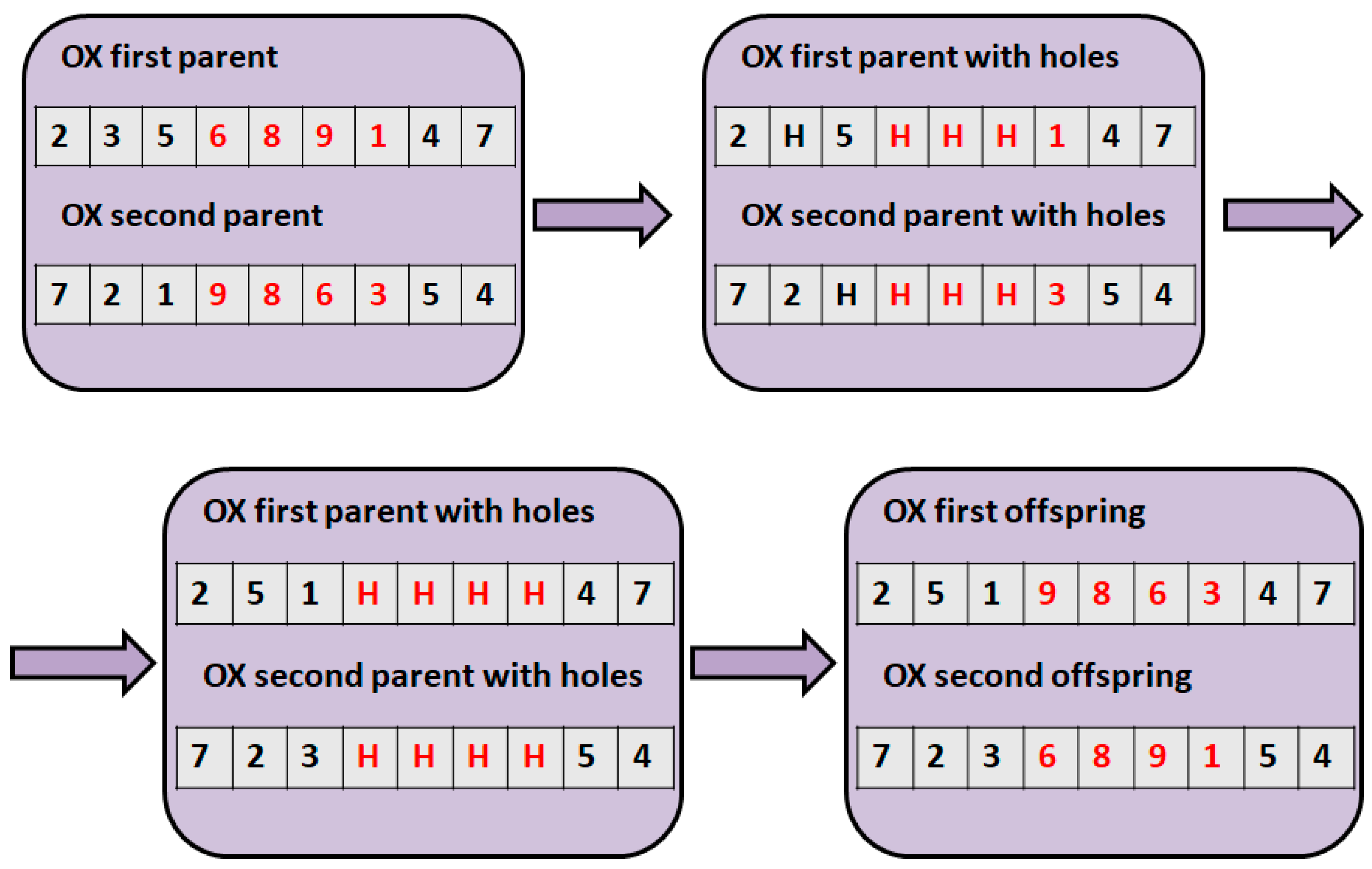
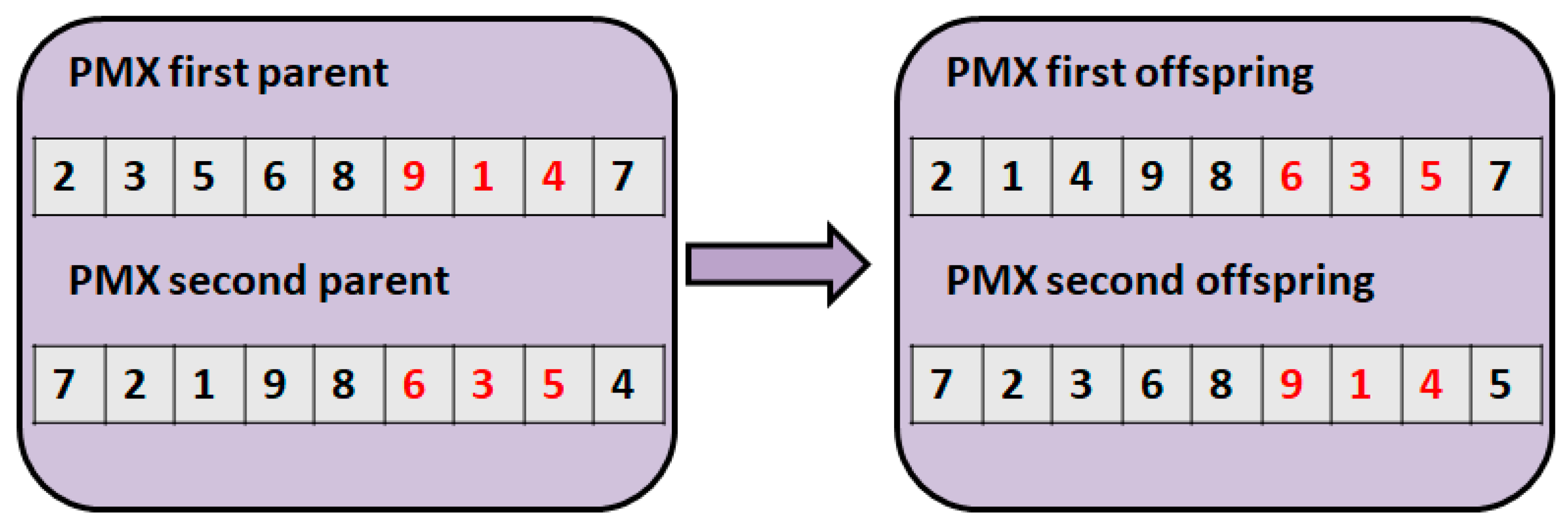
2.2. Genetic Algorithm

Genetic algorithm [16] is a general optimization algorithm. The algorithm maintains a population of solutions. In the genetic algorithm, the elements of a population are called individuals. After generating the initial population, the algorithm attempts to improve the population in each iteration with operations such as mutation and crossover. The mutation maintains a small change in each individual. An example of such a mutation is the 2-opt operation. During crossover (such as cycle crossover, partially matched crossover, order crossover etc.), two children individuals are usually created from two parent individuals. In each iteration, it is even important to decide which individuals will be transferred to the population of the next iteration, this is called selection (Table 2).

2.3. Search Space in TSP

Optimization metaheuristics are based on navigation iterations in the search space. The body of the iteration cycle is based on the following elements [49,50]:
  • The set of possible states denoted by S . The search space can be discrete or continuous.
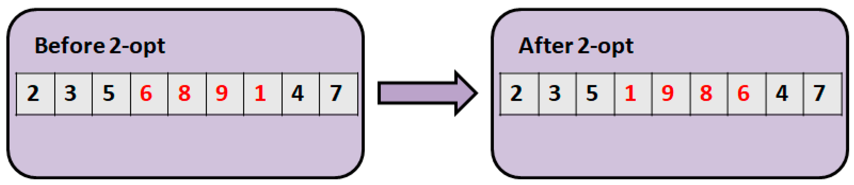
  • Distance-based neighborhood defined by an operator. This is applied to the current state point to generate the next state point. For example, for discrete problems, the edge swap (2-opt) operator. It can be written with the following notation: N x P ( x ) .
  • Fitness value, objective function denoted by f S R . This gives the fitness value for each possible status point (solution). Usually, fitness is a real number. For most optimization tasks, we use a single fitness value. However, in multi-object optimization, the fitness value may be a vector.
  • Encoding and representation: Although encoding and representation are not formally part of the fitness landscape, they are important factors. This is because representation is part of the evaluation of fitness value, and mutation operators depend on representation.
  • Transition rule (transition rule = pivoting rule = selection strategy) that selects the next state point from the potential neighboring state points.
  • Stop condition, which determines when the algorithm terminates.
  • The initial state point is either a randomly generated solution (state point) or a solution given by some construction heuristic.
The formal description of the fitness landscape can be summarized as follows [49]:
F ( S , f , N ) .
Relationship between fitness landscape analysis and optimization algorithms is the following: optimization algorithms look for a good search space state in a relatively low (minimal) time, while fitness landscape analysis provides a good insight into the problem in a minimal amount of time. Looking into the fitness landscape can be a good technique for developing new optimization algorithms [49].
The purpose of fitness landscape analysis is exploring the geometric properties of the fitness landscape, showing the efficiency of local search algorithms. Mapping this property helps to draw the following conclusions [51]:
  • Comparison of differences between two search spaces: a task with two or more different representation methods: different representation, different mutation operator, different objective function, etc.
  • Algorithm selection: analysis of the global geometry of the search space (landscape).
  • Tuning the parameters.
  • Controlling parameters during the running.

2.4. Fitness Cloud

A fitness cloud is a figure that contains the fitness value of the “base” state point and the fitness values of the neighboring states of the “base” state point (bordering fitness) [32,49].
For each search space state point (solution candidate), it represents a point in the coordinate system, where the x-axis represents the fitness value of the “base” state and the y-axis represents the fitness value of the neighbor state of the “base” state point. Formally, F C = { ( f ( x ) , f ˜ ( x ) ) | x S } , where the fitness value of the “base” state is denoted by f , while the fitness value of the “adjacent” (bordering) state is denoted by f ˜ . We introduce the sets F C m i n ,   F C m e a n ,     F C m a x , which can be defined as follows [34]:
F ( S , f , N ) F C m i n { ( ϕ , ϕ ˜ ) | ϕ f ( S ) ,   ϕ ˜ = min x S ϕ f ˜ ( x ) } F C m e a n { ( ϕ , ϕ ˜ ) | ϕ f ( S ) ,   ϕ ˜ = mean x S ϕ f ˜ ( x ) F C m a x { ( ϕ , ϕ ˜ ) | ϕ f ( S ) ,   ϕ ˜ = max x S ϕ f ˜ ( x ) .
Let φ be the fitness value of the “base” state point, α be the associated F C m i n value, β be the associated F C m e a n value, and γ be the associated F C m a x value.
Then, we can perform the following study based on it for a maximization task [49]:
  • φ < α : If the fitness value of the “base” state point is below α , then the bordering fitness values are better, so we call it strictly advantageous.
  • α < φ β : If the fitness value of the “base” state point is between α and β , it is called average advantageous because the bordering fitness values are higher than theirs.
  • β < φ γ : The “base” fitness point value between β and γ is called deleterious because their average bordering fitness value is lower than the “base” fitness point value.
  • γ < φ : A “base” fitness value above γ is called strictly deleterious because their bordering fitness is always lower than themselves.

3. Proposed Analysis and Optimization Methods

3.1. Proposed Neighborhood Operators

The structure of the fitness landscape is greatly influenced by the neighborhood operator, as the main goal of fitness landscape analysis is to prove the efficiency of the algorithms. Four operators were used in the analyses, as follows: 2-opt, cycle crossover, order crossover, partially matched crossover.
Figure 2 presents the 2-opt [52] operator. This operator operates on one solution. A section is chosen, and the elements are exchanged. This means an exchange of two edges.
Figure 3 illustrates the cycle crossover (CX) [16]. During this method, we search for cycles. Initially, the first offspring gets the first position of the first parent, and the second offspring gets the first position of the second parent. In our example, the first offspring gets 2 and the second offspring gets 7. After that, the second offspring has 7, so the first offspring must also have 7. Therefore, the first offspring gets 7 in the appropriate position, and the second offspring gets 4 in the appropriate position. After that, the (4,5) pairs are chosen, then the (5,1), (1,3), (3,2). After (3,2) is chosen, the circle closed. As the last step, the first offspring gets the numbers from the second parent in the remainder position, and the second offspring gets the numbers from the first parent.
Figure 4 illustrates the order crossover (OX) [16]. In the case of this crossover, a fitting section is determined. The length and the position of the fitting section of the two parents must be the same. After that, the parents are copied, these are initially the two offsprings. In the first offspring, we look for the numbers that the second parent fitting section contains. These numbers are deleted, indicated with H letter in Figure 4. In the second offspring, we look for the numbers that the first parent fitting section contains. After that, the holes (H letters) are pushed up to the fitting section. In the fitting section, the holes are replaced with the following way: the first offspring gets the fitting section of the second parent, and the second offspring gets the fitting section of the first parent.
Figure 5 illustrates the partially matched crossover (PMX) [16] technique. In the case of this technique, a fitting section is determined. These fitting sections of the two parents must have the same length and positions. After that, pairs are created from the fitting section. In this example, the pairs are the followings: (9,6), (1,3), and (4,5). The creation of the offspring is the following: we copy the parents. After that, the elements of the pairs are exchanged. In our example, the 6 is exchanged with 9, the 1 is exchanged with 3, and the 4 is exchanged with 5.

3.2. Measuring Distances between Two Solutions

For measuring distances between two state points, we use the following three techniques: fitness distance, Hamming-distance, and basic swap sequence distance. Figure 6 illustrates an example of measuring distances between two state points.
The fitness distance is the absolute value of the fitness value differences between the two state points. In our example (Figure 6), |1500−1000| = 500 will be the value, because the fitness value of the first solution is 1500 and the fitness value of the second solution is 1000.
The Hamming distance [53] is the number of differences in the representation of the two state points. In our example (Figure 6), the two solutions differ in the following positions: position 4, position 5, position 6, position 7. These represent the following pairs: position 4: (6,1), position 5: (8,9), position 6: (9,8), position 7: (1,6).
The basic swap sequence [54] is the number of exchanges between two state points. In our example (Figure 6), we can get solution 2 from solution 1 with a single edge change (2-opt operator). This is the reverse of the sequence (6,8,9,1).

3.3. Key Performance Indicators in Our Fitness Cloud Analysis

In this chapter, we present fitness cloud indicators and our proposed evaluation strategy. The following indicators were used:
Fitness values (for the entire cloud) of the entire solutions (base and neighbor) are evaluated. Fitness values, because we have a minimization task, need to be small but move around a large range of values so they can effectively map the search space.
Average of fitness distances, where the distances were taken from the base and neighbor solutions, and then these distances were averaged to obtain an average distance for each base solution.
Average of Hamming distances shows aggregated distances, also from base and neighbor solutions, while the average of basic swap sequence distances was also calculated. The average Hamming and basic swap sequence distances should be large to map the effective search space.
FC-max, FC-mean, and FC-min values are determined for all base points. FC-max values are the maximum values of the neighbor solutions, while FC-mean values are the means of the neighbors and FC-min values are the min of the neighbor fitnesses. The FC-max values since minimization is a task, so the lower the values, the better the operator. FC-mean measures the average of the bordering solution, the goal is to obtain solutions with good average fitness value (low fitness value in case of minimization task). The FC-min value is the maximum fitness of the bordering solutions (in the case of a minimization task), this value can be high, so the operator can better map the search space.
The strictly advantageous count indicates that the fitness values of the neighbors are lower than the fitness value of the given solution. The higher this value, the better the operator.
An average advantageous count indicates that the bordering fitness values are better than the base fitness values on average. The higher this value, the better the operator.
Average deleterious count indicates that the bordering fitness values are worse than the base fitness values on average. If this value is 0 or very small, the operator is efficient.
Strictly deleterious count indicates that the bordering fitness values are worse than the base fitness values. If this value is 0 or very small, the operator is efficient. The calculation of the key indicators can be seen in Table 3.

3.4. Edge Weighting-Based Optimization for Traveling Salesman Problem

The heuristic methods for TSP usually are based on the idea to generate a route population and award such route sections which are contained in routes with high fitness value. In GA, for example, the selection and crossover operators are used to highlight important route sections. The GA method starts with the generation of the initial population and then it performs an iteration to improve the population by generating new items using the standard GA operators.
On the other hand, our analysis of the fitness cloud has been proved that the classical crossover operations are not the best operators to improve the fitness value. Thus, many variants of evolutionary algorithms were proposed to involve some variant of the 2-opt operators besides the classical crossover, selection, and mutation operators.
The main motivation behind our proposed model is to improve the selection process of the optimal route sections using a more direct way. In GA, the route sections are somehow latent, the selection depends on many random elements. In contrast with this approach, the proposed model provides an explicit route segment selection.
In this section, we present a novel approach which can provide similar flexibility as the 2-opt operator. The proposed model is based on the following background ideas:
  • Application of edges as elementary units in the route construction process; this approach provides higher flexibility.
  • Introduction of a fitness value also for the elementary, edges based on their role in routes with high fitness values. The approach to score elementary units can be found among others in the Bayes-classifiers where every component attribute is assigned to a probability weight value.
The proposed algorithm investigates only short route sections connecting neighboring elements. The importance of a section is measured with the fitness of the container routes. During the construction of routes, the engine prefers the neighborhoods with high fitness values.
The proposed optimization model is based on the following formalism.
  • O = { o i } : set of objects (locations);
  • D = { d i j = d ( o i , o j ) } : set of distances between the objects;
  • P = { p i } : set of closed permutations, closed routes on O ;
  • l ( p ) : the length of closed route p ;
  • f ( p ) : the fitness of closed route p .
We introduce the notation N k ( o 1 , o 2 ) to denote the case that the distance between o1 and o2 in a given route is smaller than k .
We can convert the ( O , D , P ) TSP problem into an information table T ( P , A ) , where A   =   { a i j } is the set of attributes.
The attribute a i j shows the nearness of the two objects o i and o j . The attribute a i j is met if o i is in the neighborhood of o j in the route.

Example

Let us take 4 objects ( o 1 , o 2 , o 3 , o 4 ) and the population contains the following three routes: p 1 ( o 1 , o 4 , o 3 , o 2 ) , p 2 ( o 1 , o 2 , o 4 , o 3 ) , p 3 ( o 1 , o 2 , o 3 , o 4 ) . If the neighborhood means direct connections (1-NN case), then we have the following information table (Table 4).
One parameter of the model is the size of the neighborhood. Usually, we take a small size between 3 and 5.
We assign a fitness value f ( a i j ) also for the attributes, where this value denotes the chance that the corresponding items are in the neighborhood, and a route with high fitness value contains the corresponding edge ( o i , o j ) . Having these attribute level fitness values, we should use the edges with high f ( a i j ) values to construct an optimal route.
The attribute level fitness value is high if N k ( o i , o j ) is frequent in routes with high fitness values, thus we use the following formula to calculate the attribute level fitness:
f ( a i j ) =   p {   w i j p   · f ( p )   |     N k ( o i , o j )   } ,  
where w i j p denotes a weight value. In the simplest, non-weighted case, w i j p = 1 . In the case of the weighted model, w i j p depends on the distance between the two objects, the larger is the distance, the smaller is the weight value.
The N k ( o i , o j ) condition means that o i and o j are in a neighborhood in the given route. The symbol   means here an aggregation operator. Based on our experience, either the Sum or the Max operators are the best candidates.
For calculation of the   f ( a i j ) values, we use a training set of the routes. The routes can be generated randomly or by using some heuristics. The optimal route candidate is generated in such a way that as many good edges as possible will be included (Table 5).

4. Results and Discussion

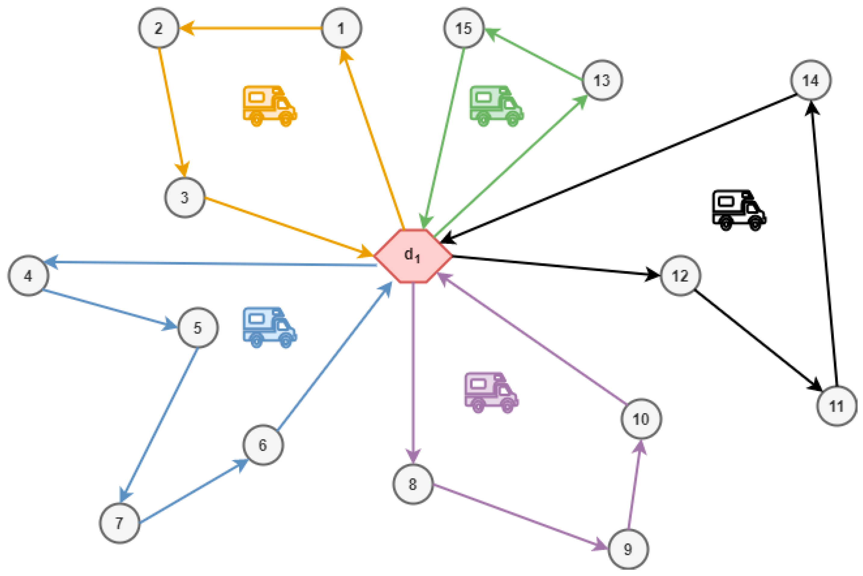
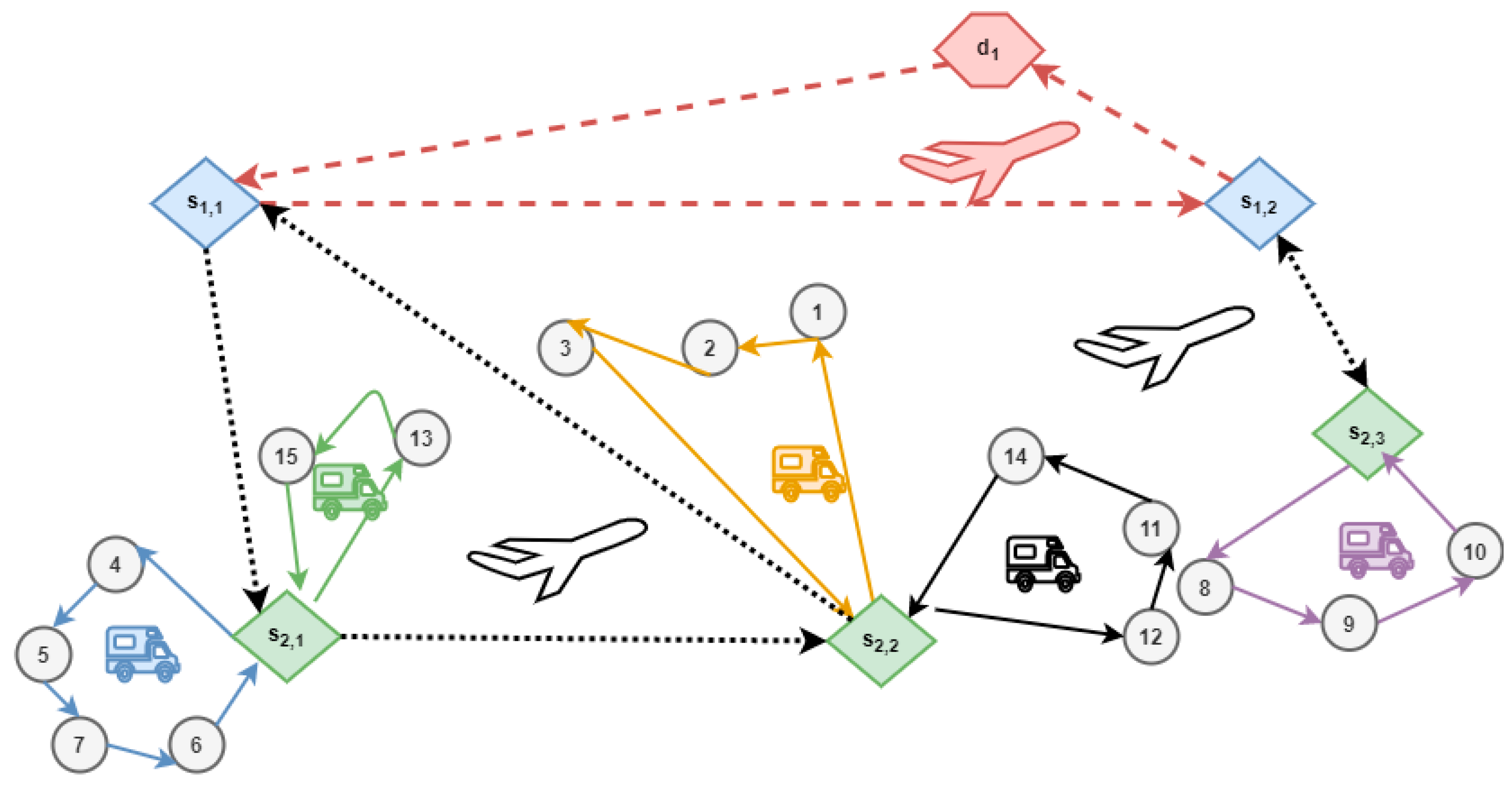
4.1. The Prototype Vehicle Routing System

Our complex vehicle routing problem, which is illustrated in Figure 7, is a multi-echelon system. Our data set is artificially generated. The system consists of depots (4 counts, the coordinates are between [0, 100]), satellites, and customers (15 counts, the coordinates are between [600, 700]). In our system, there are first (10 counts, the coordinates are between [200, 300]) and second level satellites (10 counts, the coordinates are between [400, 500]). The products are transported from the depots to the first level satellites, then to the second level satellites, after that to the customers, because the customers have product demands, which vary along with customers. In each level, there are different types of vehicles (2 types of vehicles per level). Our system consists of only one product type. Each vehicle has a different capacity limit (for the products) between [10,000, 50,000], and the vehicles have different fuel consumptions [10, 100]. In our system, not only the travel distances between the locations (which depends on the coordinates of the locations) are important, but also the travel time (between [10, 100]) and the route status between the nodes (between [100, 500]). These factors vary along with locations and vehicles. In connection with the delivery of the products, we have also defined some temporalities that occur in the nodes. These temporalities are the following: the loading (between [30, 50]) and unloading time (between [30, 50]), and the administration time (between [30, 50]). These components vary along with locations and vehicles. Our system also contains cost in connection with the transportation of products. These costs are the following: loading (between [10, 50]) and unloading cost (between [10, 50]), administrative (between [10, 50]), and quality control cost (between [10, 50]). These costs vary along with locations and vehicles. Our objective function is not only the minimization of the length of the route, but the minimization of the fuel consumption of the vehicles, maximization of the route status, minimization of the route time, and minimization of the missed (unvisited) customers. Based on our analysis, the typical size (the number of nodes) of the related TSP problems is near 100. This means that the optimization algorithm should focus on the middle-size problem domain.

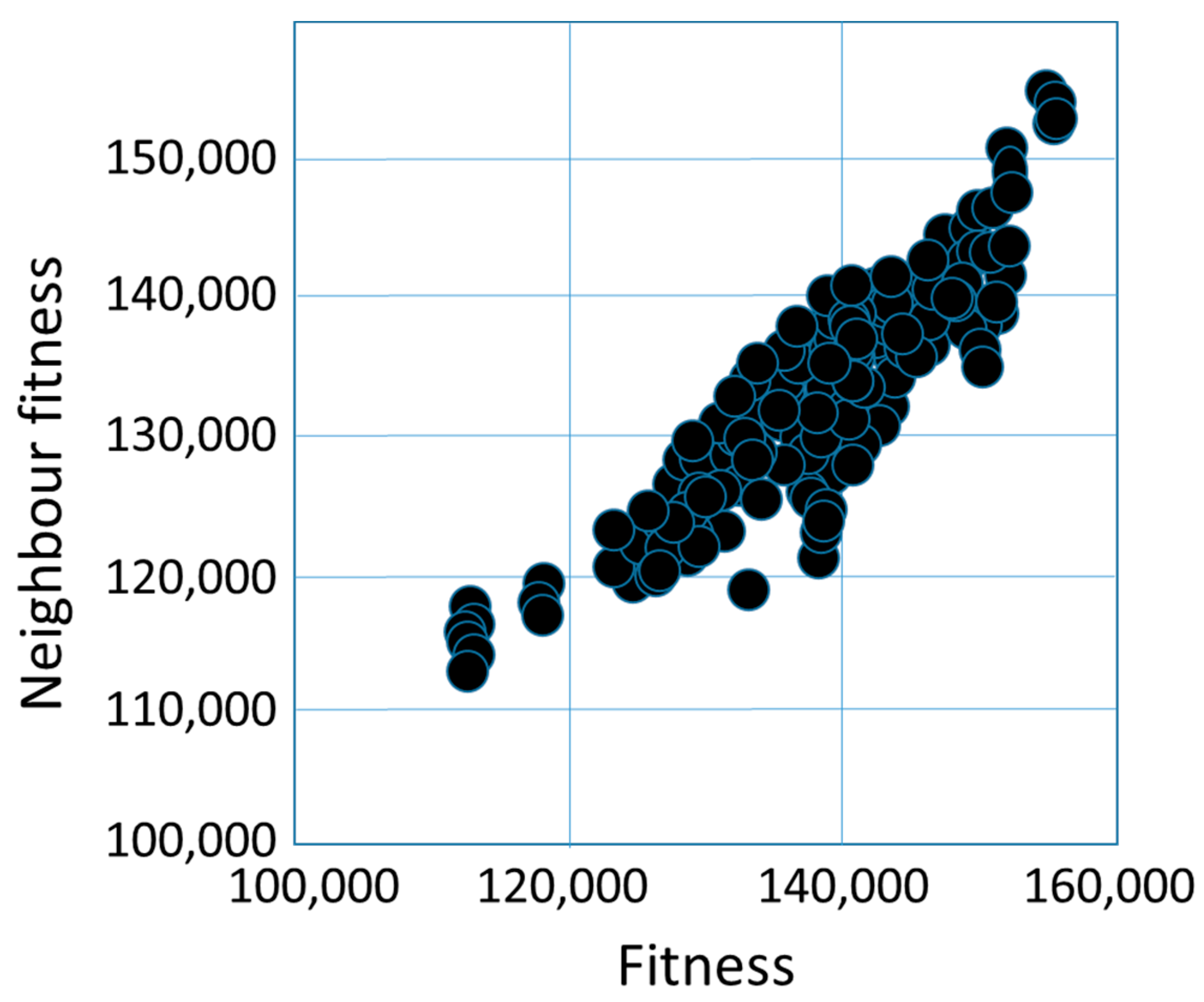
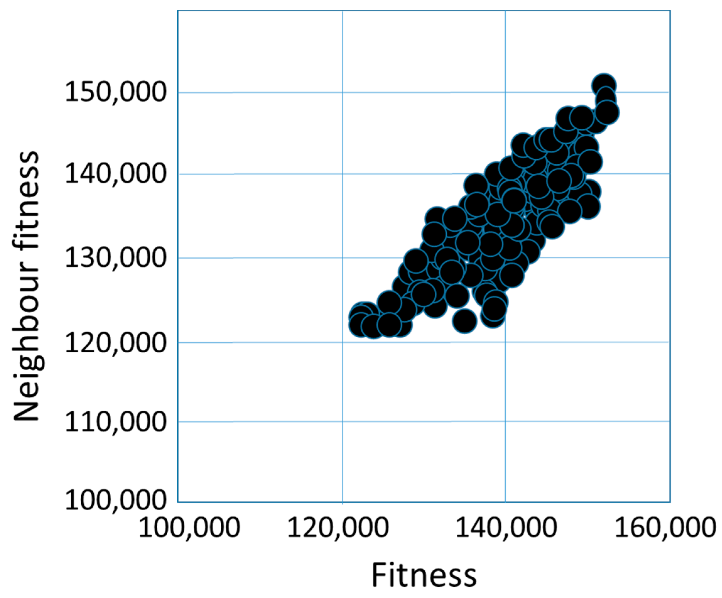
4.2. Fitness Cloud Analysis Results

In this section, the fitness cloud of our multi-echelon VRP model in the case of different operators are presented. During the creation of the fitness cloud, we randomly select solutions and then create their neighbors. The representation of the solutions and the neighbors, their relation to them is important in the analysis. The following analysis techniques were used: fitness cloud, Fc-max, Fc-min, Fc-mean, strictly advantageous count, average advantageous count, average deleterious count, strictly deleterious count. The following operators are analyzed: 2-opt, order crossover (OX), cycle crossover (CX), partially matched crossover (PMX).
Figure 8 illustrates the fitness cloud for the 2-opt operator. Fitness values range from 100,000 to 150,000. Neighbors with lower fitness value solutions also have lower fitness values, while those with higher fitness value solutions also have higher fitness values. Table 6 illustrates that the average of fitness distances between the solutions ranges between 2500 and 9000 values, and the average of Hamming distances ranges between 27 and 35, and the averages of basic swap sequence distances are between 21 and 27. Averages were calculated for the total fitness cloud. We calculated the averages with the following way: we looked at the distance of each solution from the other solutions and averaged this.
Figure 9 illustrates the fitness cloud for the OX operator. Fitness values range from 120,000 to 150,000. Here, too, it is typical that the fitness values of the neighbors of solutions with lower fitness values are also lower, while the fitness values of the neighbors of solutions with higher fitness values are also higher. Table 7 illustrates that the average of fitness distances between the solutions ranges between 2000 and 10,000 values, and the average of Hamming distances ranges between 31 and 35, and the averages of basic swap sequence distances are between 22 and 29.
Figure 10 illustrates the fitness cloud for the CX operator. Fitness values range from 110,000 to 160,000. Here, too, it is typical that the fitness values of the neighbors of solutions with lower fitness values are also lower, while the fitness values of the neighbors of solutions with higher fitness values are also higher. Table 8 illustrates, that the average of fitness distances between the solutions ranges between 1800 and 5000 values, and the average of Hamming distances ranges between 24 and 32, and the averages of basic swap sequence distances are between 19 and 23.
Figure 11 illustrates the fitness cloud for the PMX operator. Fitness values range from 120,000 to 160,000. Here, too, it is typical that the fitness values of the neighbors of solutions with lower fitness values are also lower, while the fitness values of the neighbors of solutions with higher fitness values are also higher. Table 9 illustrates, that the average of fitness distances between the solutions ranges between 2000 and 75,000 values, and the average of Hamming distances ranges between 29 and 35, and the averages of basic swap sequence distances are between 22 and 28.
FC-max values are lower for solutions with lower fitness values, while FC-max values are also higher for solutions with higher fitness values for all operators.
The FC-mean values are lower for solutions with lower fitness values, while the FC-mean values are also higher for solutions with higher fitness values for all operators.
The FC-min values are lower for solutions with lower fitness values, while the FC-min values are also higher for solutions with higher fitness values for all operators.
Strictly advantageous count values was the best for 2-opt, which means that the fitness values of the neighbors are lower than the fitness value of the given solution, which proves the goodness of the operator, since our task is a minimization problem.
The average advantageous count values for 2-opt is the highest, which means, that the bordering fitness values are better than the base fitness values on average.
The average and strictly deleterious counts are high for partially matched crossover, order crossover, and cycle crossover, which means that these operators are worse than 2-opt. The strictly deleterious count was high in the case of partially matched crossover and order crossover.
For the fitness cloud measurement, we summarize the results in Table 10. According to the table, the 2-opt operator became efficient, the partially matched crossover operator according to this measurement did not become as efficient as the other operators (order crossover, partially matched crossover).
According to the fitness cloud, 2-opt fitness values are the lowest values ( 100,000– 150,000) and partially matched crossover ( 120,000– 160,000) values are the highest, so in the table, we denote that 2-opt is efficient, and PMX is not so efficient based on the fitness cloud illustration.
Typically, solutions with lower fitness values also have lower FC-max values, while solutions with higher fitness values also have higher FC-max values. For solutions with a lower fitness value, the FC-mean values are also lower, while for solutions with a higher fitness value, the FC-mean values are also higher. For solutions with lower fitness values, the FC-min values are also lower, while for solutions with higher fitness values, the FC-min values are also higher. According to them, the 2-opt operator became the best based on these measurements, the partially matched operator the worst, so in the table we denote that 2-opt is efficient in terms of FC-max, FC-mean, and FC-min, while PMX is weak in terms of these measurement strategies.
The strictly deleterious count, average deleterious count, average advantageous count, and strictly advantageous count values are nearly the same, the average advantageous count values are high for all operators, so each operator is efficient, also indicated in Table 7.

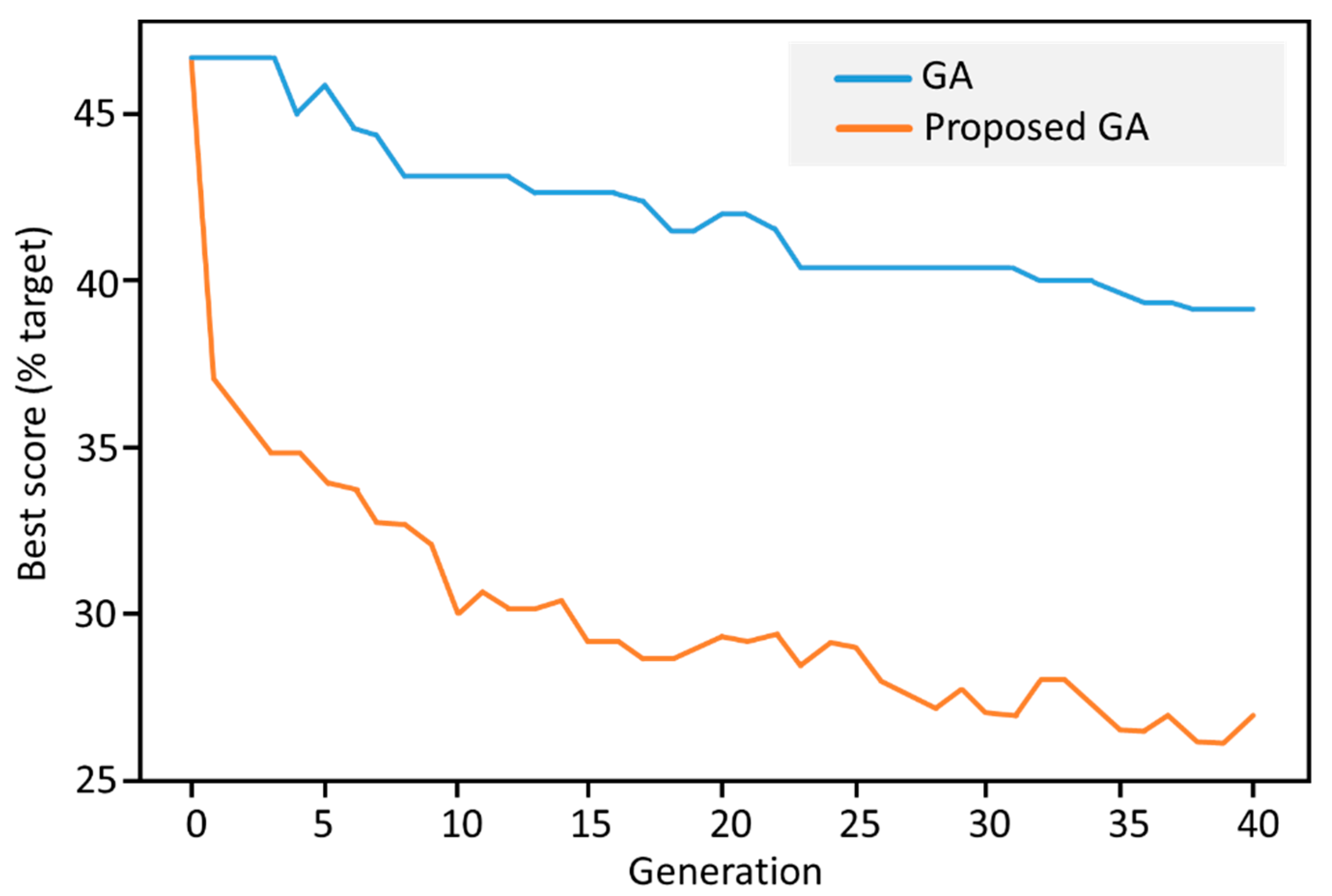
4.3. Efficiency Comparison of the Proposed Genetic Algorithm Method

Besides the simple phase route generation, we have developed an evolutional version too. In this variant, many generations are constructed using the previous generation as base set. In the proposed algorithm, first, we generate the ordered list of the edges. In the next step, we construct a random noise vector which is used to relocate some edges in the list. This means that some edges with lower values will get a higher priority while some shorter edges are assigned to lower priority. This step can be used to add random elements into the route construction process.
Having a relocation vector, the corresponding route can be generated unambiguously. In the evolutionary process, these relocation vectors are considered as gene description vectors. The population consists of a set of relocation vectors. In the iteration phase, we apply the usual selection, crossover, and mutation operators to generate the consecutive population generations.
In the corresponding GA process, the following parameters are used to adjust the algorithm:
  • N: number of the nodes;
  • P: size of the population ;
  • M: number of the generations;
  • d: relocation size;
  • p1: probability of selection;
  • p2: probability of crossover;
  • p3: probability of mutation.
The relocation size denotes the largest distance in the relocation both forward or backward. In the implemented algorithm, the (p1,p2) values are adjusted dynamically, their values are decreased if the engine could not improve the best route length in the current time window (Table 11).

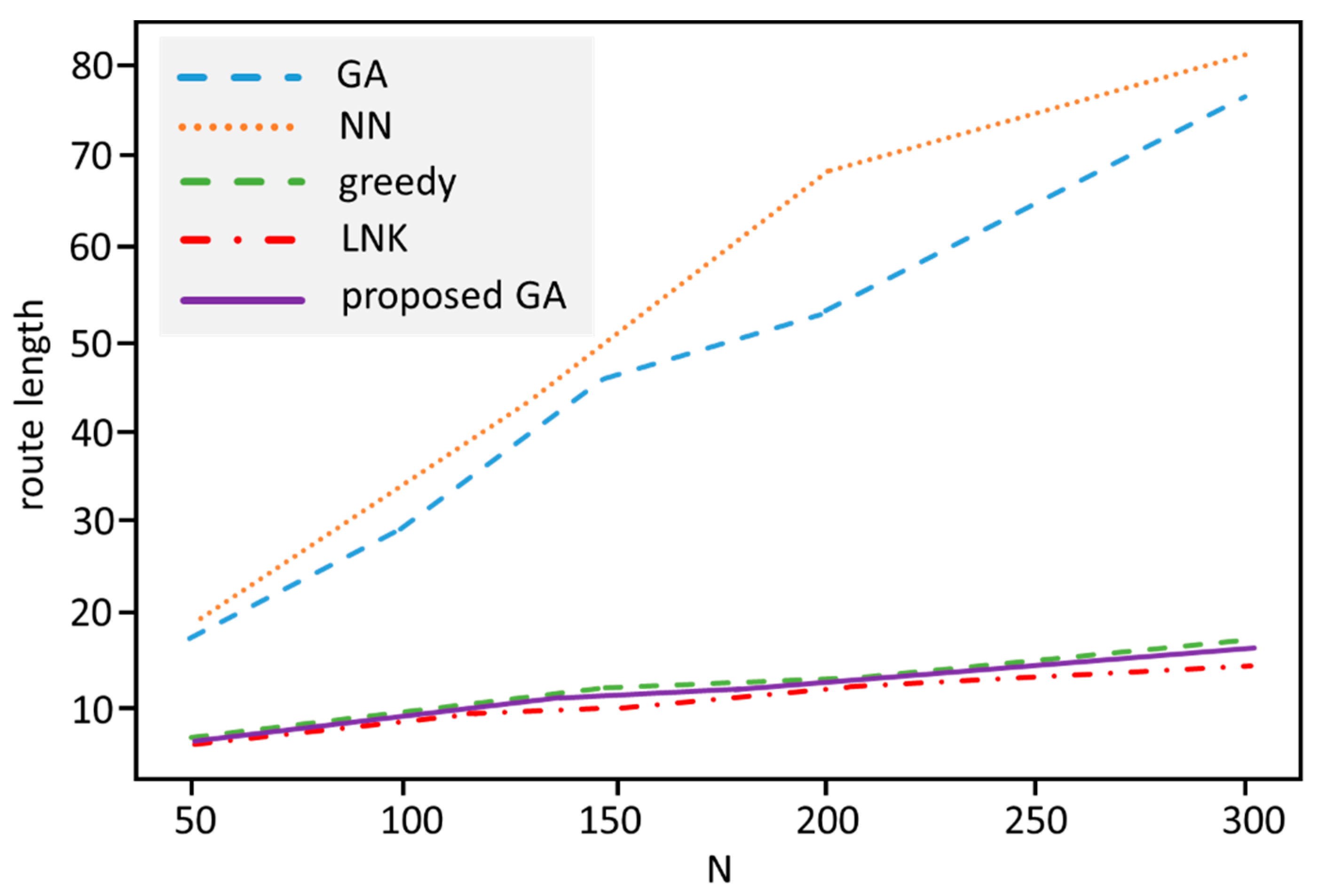
4.4. Test Results for the Proposed GA Optimization

The proposed optimization algorithms were implemented in the Python programming language. The benefit of the Python language is the availability of many different TSP solution methods on the Internet.
We involved the following methods in the efficiency comparison tests:
  • random generation (A);
  • standard GA evolutionary algorithm (B);
  • nearest neighbor construction algorithm (C);
  • greedy best first construction algorithm (D);
  • Lin-Kernighan 2-opt refinement algorithm (E);
  • proposed edge weighting single-phase (construction) algorithm (F);
  • proposed edge weighting evolutionary algorithm (G).
In the tests, according to our preliminary analysis, we used training sets in size range 50 and 200. We have used synthetic data; thus, we could generate data sets of different shapes in an easy way. The related test results are presented in Table 12. The corresponding execution time values are given in Table 13.
In the table, the following parameter notations are used:
  • N: number of nodes;
  • P: size of the population;
  • D: noise variability (only for G);
  • M: number of generations.
The experiments show that the proposed GA variant dominates the standard GA, NN, and greedy algorithms in general. An interesting result is that our method can provide better results as the efficient Lin-Kernighan method for middle-sized datasets (Figure 12 and Figure 13).
The above described approach can support the optimization of logistics systems. The design and optimization of logistics systems and supply chain solution have become more and more important because of the increased globalization of manufacturing and service processes. The design of logistics systems includes a wide range of design tasks, like layout planning, scheduling, queueing, or routing. Traveling salesman problem represents one of the core design problems of logistics systems, therefore our proposed GA optimization can improve the efficiency of solution algorithms both for internal routing problems (like in-plant, milk-run-based, material supply) and for external routing of transportation equipment.

5. Conclusions and Future Work

In this paper, we have analyzed an approach to use fitness landscape analysis in VRP/TSP to determine the optimal optimization method. In the presented prototype system, we have investigated middle-sized VRP/TSP problem domains using synthetic random input spaces. We used the fitness landscape method to analyze the search space of the prototype VRP/TSP problem. In this domain area, the performed model calculations show that 2-opt, local improvement operators dominate the global crossover operations. This experiment confirms the practical experiences found in the literature on the superiority of the 2-opt, Lin-Kernighan methods. On the other hand, 2-opt, Lin-Kernighan methods are very specialized on the TSP problem, using TSP-specific operators. Thus, we have selected the very popular GA method as a baseline evolutionary method. The purpose of our work on GA was to develop a novel approach to use local optimization operators instead of global crossover steps. The proposed method is based on the application of edge-level weighting in the input domain. The presented approach has some similarity with the greedy construction method, but there are some fundamental differences between the two approaches as:
  • the proposed method involves some stochastic components;
  • the proposed method uses an evolutionary framework.
The test results on the prototype system show some interesting conclusions:
  • The proposed integrated GA method provides significantly better results as the baseline GA method.
  • The experiments show that the proposed GA variant dominates the NN and greedy algorithms in general. An interesting result is that our method can provide better results as the efficient Lin-Kernighan method for middle-sized datasets.
  • The convergence and efficiency of random operations is relatively low in large problem domains where the number of possible states is exponentially high.
Based on the experiences, we can suggest the updated GA version using a greedy initialization module. This kind of engine can provide a near-optimal route length in the investigated problem range.

Author Contributions

Conceptualization, L.K. and A.A.; methodology, L.K., A.A. and T.B.; software, A.A.; validation, L.K. and A.A.; formal analysis, L.K. and A.A.; investigation, L.K. and A.A.; resources, T.B.; data curation, L.K., A.A.; writing—original draft preparation, L.K., A.A. and T.B.; writing—review and editing, L.K., A.A. and T.B.; visualization, L.K., A.A. and T.B.; supervision, L.K. and T.B.; project administration, L.K. and T.B.; funding acquisition, T.B. All authors have read and agreed to the published version of the manuscript.

Funding

The described article was carried out as part of the EFOP-3.6.1-16-2016-00011 “Younger and Renewing University—Innovative Knowledge City—institutional development of the University of Miskolc aiming at intelligent specialization” project implemented in the framework of the Szechenyi 2020 program. The realization of this project is supported by the European Union, co-financed by the European Social Fund.

Conflicts of Interest

The author declares no conflict of interest.

References

  1. Dantzig, G.B.; Ramser, J.H. The truck dispatching problem. Manag. Sci. 1959, 6, 80–91. [Google Scholar] [CrossRef]
  2. Skrlec, D.; Filipec, M.; Krajcar, S. A heuristic modification of genetic algorithm used for solving the single depot capacited vehicle routing problem. In Proceedings of the Intelligent Information Systems, Grand Bahama Island, Bahamas, 8–10 December 1997; pp. 184–188. [Google Scholar]
  3. Nagy, G.; Salhi, S. Heuristic algorithms for single and multiple depot vehicle routing problems with pickups and deliveries. Eur. J. Oper. Res. 2005, 162, 126–141. [Google Scholar] [CrossRef] [Green Version]
  4. Crainic, T.G.; Perboli, G.; Mancini, S.; Tadei, R. Two-echelon vehicle routing problem: A satellite location analysis. Procedia-Soc. Behav. Sci. 2010, 2, 5944–5955. [Google Scholar] [CrossRef] [Green Version]
  5. Dondo, R.; Méndez, C.A.; Cerdá, J. The multi-echelon vehicle routing problem with cross docking in supply chain management. Comput. Chem. Eng. 2011, 35, 3002–3024. [Google Scholar] [CrossRef]
  6. Dondo, R.; Cerdá, J. A cluster-based optimization approach for the multi-depot heterogeneous fleet vehicle routing problem with time windows. Eur. J. Oper. Res. 2007, 176, 1478–1507. [Google Scholar] [CrossRef]
  7. Gendreau, M.; Laporte, G.; Musaraganyi, C.; Taillard, É.D. A tabu search heuristic for the heterogeneous fleet vehicle routing problem. Comput. Oper. Res. 1999, 26, 1153–1173. [Google Scholar] [CrossRef]
  8. Schulze, J.; Fahle, T. A parallel algorithm for the vehicle routing problem with time window constraints. Ann. Oper. Res. 1999, 86, 585–607. [Google Scholar] [CrossRef]
  9. Belhaiza, S.; Hansen, P.; Laporte, G. A hybrid variable neighborhood tabu search heuristic for the vehicle routing problem with multiple time windows. Comput. Oper. Res. 2014, 52, 269–281. [Google Scholar] [CrossRef]
  10. Figliozzi, M.A. An iterative route construction and improvement algorithm for the vehicle routing problem with soft time windows. Transp. Res. Part C Emerg. Technol. 2010, 18, 668–679. [Google Scholar] [CrossRef]
  11. Ralphs, T.K.; Kopman, L.; Pulleyblank, W.R.; Trotter, L.E. On the capacitated vehicle routing problem. Math. Program. 2003, 94, 343–359. [Google Scholar] [CrossRef]
  12. Kabcome, P.; Mouktonglang, T. Vehicle routing problem for multiple product types, compartments, and trips with soft time windows. Int. J. Math. Math. Sci. 2015, 126754. [Google Scholar] [CrossRef] [Green Version]
  13. Crevier, B.; Cordeau, J.F.; Laporte, G. The multi-depot vehicle routing problem with inter-depot routes. Eur. J. Oper. Res. 2007, 176, 756–773. [Google Scholar] [CrossRef]
  14. Lin, C.K.Y. A vehicle routing problem with pickup and delivery time windows, and coordination of transportable resources. Comput. Oper. Res. 2011, 38, 1596–1609. [Google Scholar] [CrossRef]
  15. Angelelli, E.; Speranza, M.G. The periodic vehicle routing problem with intermediate facilities. Eur. J. Oper. Res. 2002, 137, 233–247. [Google Scholar] [CrossRef]
  16. Hussain, A.; Muhammad, Y.S.; Nauman Sajid, M.; Hussain, I.; Mohamd Shoukry, A.; Gani, S. Genetic algorithm for traveling salesman problem with modified cycle crossover operator. Comput. Intell. Neurosci. 2017, 7430125. [Google Scholar] [CrossRef] [PubMed]
  17. Stewart, W.R., Jr.; Golden, B.L. Stochastic vehicle routing: A comprehensive approach. Eur. J. Oper. Res. 1983, 14, 371–385. [Google Scholar] [CrossRef]
  18. Gupta, R.; Singh, B.; Pandey, D. Multi-objective fuzzy vehicle routing problem: A case study. Int. J. Contemp. Math. Sci. 2010, 5, 1439–1454. [Google Scholar]
  19. Soysal, M.; Bloemhof-Ruwaard, J.M.; Bektaş, T. The time-dependent two-echelon capacitated vehicle routing problem with environmental considerations. Int. J. Prod. Econ. 2015, 164, 366–378. [Google Scholar] [CrossRef]
  20. Lin, J.; Zhou, W.; Wolfson, O. Electric vehicle routing problem. Transp. Res. Procedia 2016, 12, 508–521. [Google Scholar] [CrossRef] [Green Version]
  21. Stavropoulou, F.; Repoussis, P.P.; Tarantilis, C.D. The vehicle routing problem with profits and consistency constraints. Eur. J. Oper. Res. 2019, 274, 340–356. [Google Scholar] [CrossRef]
  22. Huang, Y.H.; Blazquez, C.A.; Huang, S.H.; Paredes-Belmar, G.; Latorre-Nuñez, G. Solving the feeder vehicle routing problem using ant colony optimization. Comput. Ind. Eng. 2019, 127, 520–535. [Google Scholar] [CrossRef]
  23. Ribeiro, G.M.; Laporte, G. An adaptive large neighborhood search heuristic for the cumulative capacitated vehicle routing problem. Comput. Oper. Res. 2012, 39, 728–735. [Google Scholar] [CrossRef]
  24. Song, B.D.; Ko, Y.D. A vehicle routing problem of both refrigerated-and general-type vehicles for perishable food products delivery. J. Food Eng. 2016, 169, 61–71. [Google Scholar] [CrossRef]
  25. Talarico, L.; Sörensen, K.; Springael, J. Metaheuristics for the risk-constrained cash-in-transit vehicle routing problem. Eur. J. Oper. Res. 2015, 244, 457–470. [Google Scholar] [CrossRef] [Green Version]
  26. Bae, H.; Moon, I. Multi-depot vehicle routing problem with time windows considering delivery and installation vehicles. Appl. Math. Model. 2016, 40, 6536–6549. [Google Scholar] [CrossRef]
  27. Battarra, M.; Erdoğan, G.; Vigo, D. Exact algorithms for the clustered vehicle routing problem. Oper. Res. 2014, 62, 58–71. [Google Scholar] [CrossRef] [Green Version]
  28. Drexl, M. Applications of the vehicle routing problem with trailers and transshipments. Eur. J. Oper. Res. 2013, 227, 275–283. [Google Scholar] [CrossRef]
  29. Xiao, Y.; Konak, A. The heterogeneous green vehicle routing and scheduling problem with time-varying traffic congestion. Transp. Res. Part E Logist. Transp. Rev. 2016, 88, 146–166. [Google Scholar] [CrossRef]
  30. Montemanni, R.; Gambardella, L.M.; Rizzoli, A.E.; Donati, A.V. Ant colony system for a dynamic vehicle routing problem. J. Comb. Optim. 2005, 10, 327–343. [Google Scholar] [CrossRef]
  31. Mattfeld, D.C.; Bierwirth, C.; Kopfer, H. A search space analysis of the job shop scheduling problem. Ann. Oper. Res. 1999, 86, 441–453. [Google Scholar] [CrossRef]
  32. Pitzer, E.; Affenzeller, M. A comprehensive survey on fitness landscape analysis. In Recent Advances in Intelligent Engineering Systems, 1st ed.; Fodor, J., Klempous, R., Suárez Araujo, C.P., Eds.; Springer: Berlin/Heidelberg, Germany, 2012; pp. 161–191. [Google Scholar] [CrossRef]
  33. Humeau, J.; Liefooghe, A.; Talbi, E.G.; Verel, S. ParadisEO-MO: From fitness landscape analysis to efficient local search algorithms. J. Heuristics 2013, 19, 881–915. [Google Scholar] [CrossRef] [Green Version]
  34. Collard, P.; Verel, S.; Clergue, M. Local search heuristics: Fitness cloud versus fitness landscape. arXiv 2007, arXiv:0709.4010. [Google Scholar]
  35. Fonlupt, C.; Robilliard, D.; Preux, P. Fitness landscape and the behavior of heuristics. Evol. Artif. 1997, 97, 56. [Google Scholar]
  36. Ventresca, M.; Ombuki-Berman, B.; Runka, A. Predicting genetic algorithm performance on the vehicle routing problem using information theoretic landscape measures. Lect. Notes Comput. Sci. 2013, 7832, 214–225. [Google Scholar] [CrossRef]
  37. Bagaria, V.; Ding, J.; Tse, D.; Wu, Y.; Xu, J. Hidden hamiltonian cycle recovery via linear programming. Oper. Res. 2020, 68, 53–70. [Google Scholar] [CrossRef] [Green Version]
  38. Papadimitriou, C.H.; Vazirani, U.V. On two geometric problems related to the travelling salesman problem. J. Algorithms 1984, 5, 231–246. [Google Scholar] [CrossRef]
  39. Braun, H. On solving travelling salesman problems by genetic algorithms. Lect. Notes Comput. Sci. 1991, 496, 129–133. [Google Scholar]
  40. Rosenkrantz, D.J.; Stearns, R.E.; Lewis, P.M., II. An analysis of several heuristics for the traveling salesman problem. SIAM J. Comput. 1977, 6, 563–581. [Google Scholar] [CrossRef]
  41. Fiechter, C.N. A parallel tabu search algorithm for large traveling salesman problems. Discret. Appl. Math. 1994, 51, 243–267. [Google Scholar] [CrossRef] [Green Version]
  42. Helsgaun, K. An effective implementation of the Lin–Kernighan traveling salesman heuristic. Eur. J. Oper. Res. 2000, 126, 106–130. [Google Scholar] [CrossRef] [Green Version]
  43. Karabulut, K.; Tasgetiren, M.F. A variable iterated greedy algorithm for the traveling salesman problem with time windows. Inf. Sci. 2014, 279, 383–395. [Google Scholar] [CrossRef]
  44. Nguyen, H.D.; Yoshihara, I.; Yamamori, K.; Yasunaga, M. Implementation of an effective hybrid GA for large-scale traveling salesman problems. IEEE Trans. Syst. Manand Cybern. Part B 2007, 37, 92–99. [Google Scholar] [CrossRef] [PubMed]
  45. Paessens, H. The savings algorithm for the vehicle routing problem. Eur. J. Oper. Res. 1988, 34, 336–344. [Google Scholar] [CrossRef]
  46. Snyder, L.V.; Daskin, M.S. A random-key genetic algorithm for the generalized traveling salesman problem. Eur. J. Oper. Res. 2006, 174, 38–53. [Google Scholar] [CrossRef]
  47. Rego, C.; Gamboa, D.; Glover, F.; Osterman, C. Traveling salesman problem heuristics: Leading methods, implementations and latest advances. Eur. J. Oper. Res. 2011, 211, 427–441. [Google Scholar] [CrossRef]
  48. Gambardella, L.M.; Dorigo, M. Ant-Q: A reinforcement learning approach to the traveling salesman problem. In Proceedings of the Twelfth International Conference on Machine Learning, Tahoe City, CA, USA, 9–12 July 1995; pp. 252–260. [Google Scholar] [CrossRef]
  49. Pitzer, E. Applied Fitness Landscape Analysis. Ph.D. Thesis, Johannes Kepler Universität Linz, Linz, Austria, 2013. [Google Scholar]
  50. Fonlupt, C.; Robilliard, D.; Preux, P.; Talbi, E.G. Fitness Landscapes and Performance of Meta-Heuristics. In Meta-Heuristics, 1st ed.; Voß, S., Martello, S., Osman, I.H., Roucairol, C., Eds.; Springer: Boston, MA, USA, 1999; pp. 257–268. [Google Scholar] [CrossRef]
  51. Verel, S. Fitness landscapes and graphs: Multimodularity, ruggedness and neutrality. In Proceedings of the 11th Annual Conference Companion on Genetic and Evolutionary Computation Conference: Late Breaking Papers, Montreal, QC, Canada, 8–12 July 2009; Association for Computing Machinery: New York, NY, USA; pp. 3593–3656. [Google Scholar] [CrossRef]
  52. Englert, M.; Röglin, H.; Vöcking, B. Worst Case and Probabilistic Analysis of the 2-Opt Algorithm for the TSP. Algorithmica 2014, 68, 190–264. [Google Scholar] [CrossRef] [Green Version]
  53. Zhu, K.Q. A diversity-controlling adaptive genetic algorithm for the vehicle routing problem with time windows. In Proceedings of the 15th IEEE International Conference on Tools with Artificial Intelligence, Sacramento, CA, USA, 5 November 2003; pp. 176–183. [Google Scholar] [CrossRef]
  54. Wang, K.P.; Huang, L.; Zhou, C.G.; Pang, W. Particle swarm optimization for traveling salesman problem. In Proceedings of the 2003 International Conference on Machine Learning and Cybernetics, Xi’an, China, 5 November 2003; pp. 1583–1585. [Google Scholar] [CrossRef]
Figure 1. The basic vehicle routing problem (VRP).
Processes 08 01363 g001
Figure 2. The 2-opt.
Processes 08 01363 g002
Figure 3. The cycle crossover (CX).
Processes 08 01363 g003aProcesses 08 01363 g003b
Figure 4. The order crossover (OX).
Processes 08 01363 g004
Figure 5. The partially matched crossover (PMX).
Processes 08 01363 g005
Figure 6. The example of measuring distances between two solutions (state points).
Processes 08 01363 g006
Figure 7. The multi-echelon system.
Processes 08 01363 g007
Figure 8. The fitness cloud for 2-opt operator.
Processes 08 01363 g008
Figure 9. The fitness cloud for order crossover operator.
Processes 08 01363 g009
Figure 10. The fitness cloud for cycle crossover operator.
Processes 08 01363 g010
Figure 11. The fitness cloud for partially matched crossover operator.
Processes 08 01363 g011
Figure 12. Convergence of the GA (Genetic Algorithm) method and the proposed method.
Processes 08 01363 g012
Figure 13. Route length in dependency of problem size for the TSP algorithms.
Processes 08 01363 g013
Table 1. The VRP types that contributed to our VRP system.
VRP TypeExplanation
Single [2] and Multiple Depot [3] VRPone or more depot
Two-Echelon [4] (Multi-Echelon [5]) VRPwith one or more additional satellites
Homogeneous [6] and Heterogeneous [7] VRPsame or different type of vehicles
Time Windows [8]: Single, Multiple [9], or Soft [10]customers must be served within one of the intervals
Capacitated VRP [11]capacity limit of the vehicles
Single Product or Multiple Product [12] VRPone or more types of products
Inter-Depot Route [13] VRPvehicles can return to any depot at the end of their route
Delivery, Pickup or Delivery and Pickup VRP [14]movement of products: from the depot to the customers, or vice versa, possibly both
Periodic VRP [15]periodic visit of customers
Traveling Salesman Problem [16]only one vehicle (agent) visits customers (cities) create a tour where the objective is to minimize the length of the trip
Table 2. Pseudo-code of the genetic algorithm.
  create the initial population
  while (termination criteria is not met) do
  calculate the fitness value of the population
   while (the next population is not completely created) do
    select parents
    apply crossover operator
    apply mutation operator
   end while
  end while
Table 3. Calculation of the key indicators.
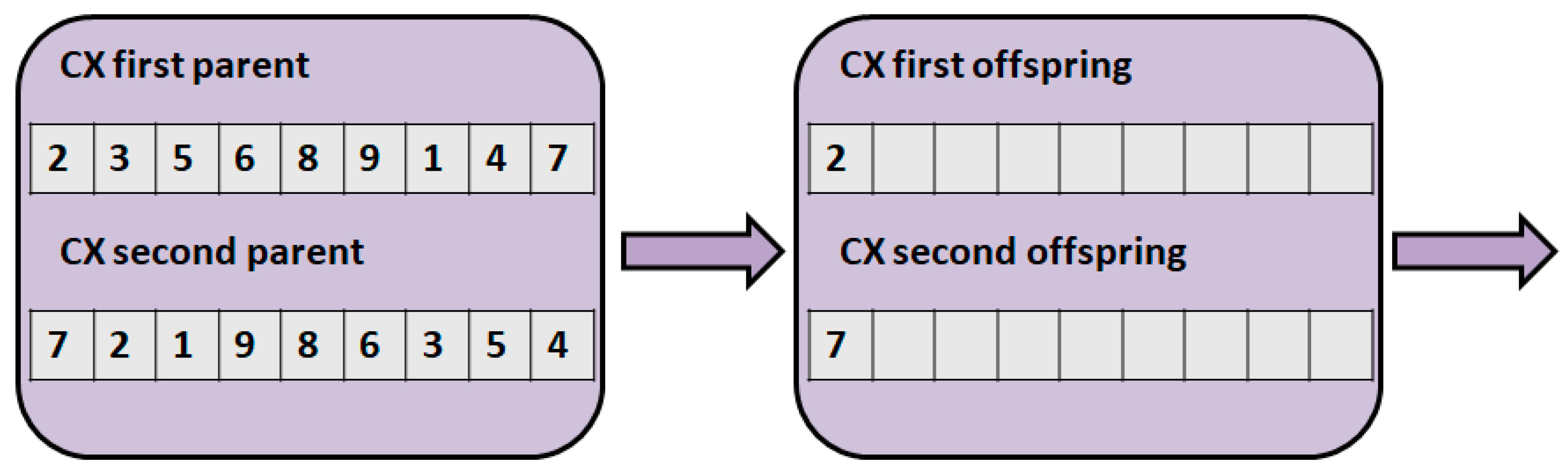
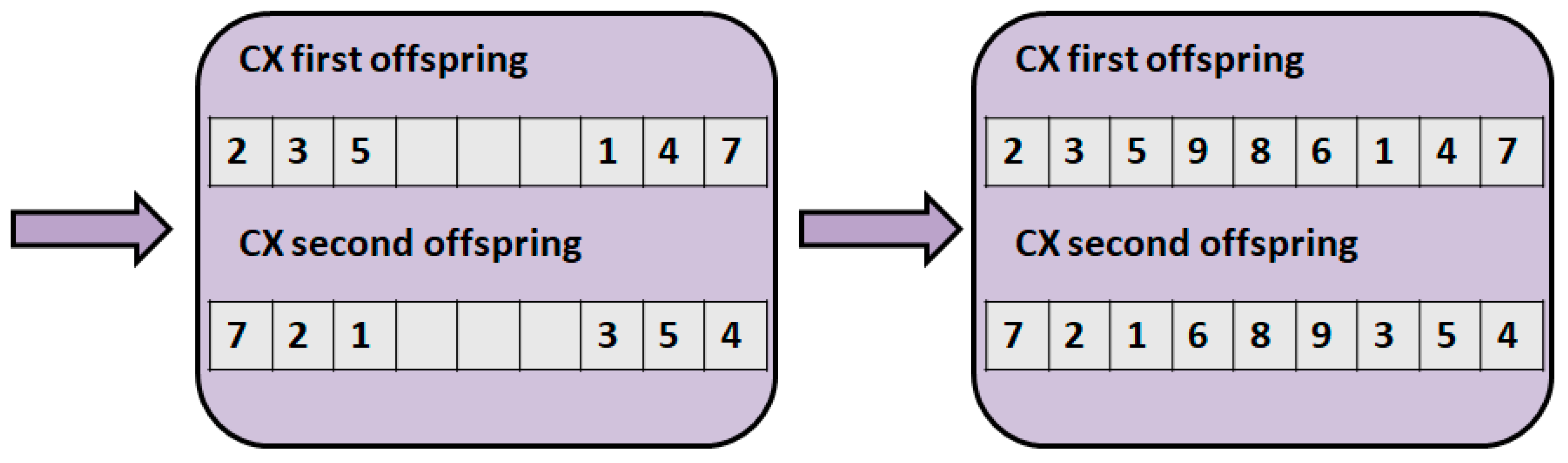
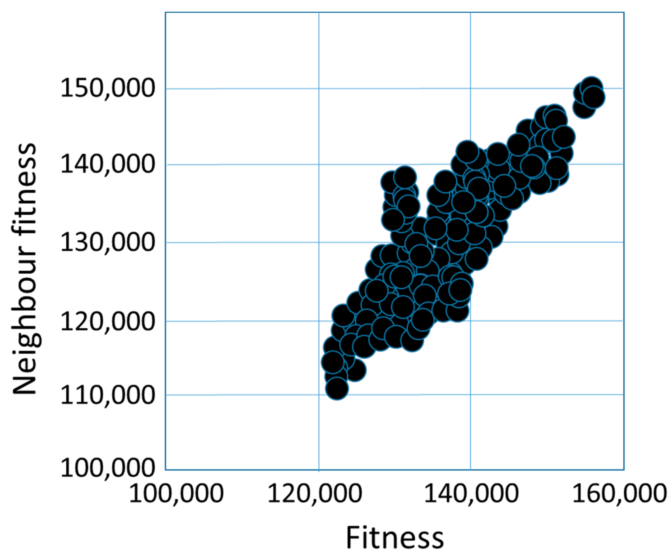
  create the initial solutions (base solutions)
  generate the neighbors of the initial solutions (with 2-opt, CX,OX, or PMX operator)
  calculate the fitness of the base solutions and their neighbors
  illustrate the fitness cloud (x-axis means the fitness of the base solution, and y-axis means the fitness of the neighbor solution)
  calculate the distances between the base solutions and their neighbors
  calculate the F C m i n , F C m e a n and F C m a x values
Table 4. Information table structure.
a 12 a 13 a 14 a 23 a 24 a 34
p 1 001101
p 2 100011
p 3 100101
Table 5. Heuristic algorithm for route generation.
  calculate fitness value for every object pairs;
  route = empty;
  process the edges in descending order by the fitness value:
    let ( o i , o j ) be the current edge;
    if o i is used already as a start point, drop this edge;
    if o j is used already as an end point, drop this edge;
    if there is a path from o j to o i , drop this edge;
    if ( o i , o j ) is a valid candidate, than merge it to the current route;
  display route.
Table 6. 2-opt distances results.
2-opt
Lower BoundUpper Bound
Fitness values 100,000 150,000
Average of fitness distances 2500 9000
Average of Hamming distances2735
Average of basic swap sequence distances2127
FC-max 110,000 150,000
FC-mean 110,000 150,000
FC-min 110,000 150,000
Value
Strictly advantageous count5
Average advantageous count34
Average deleterious count54
Strictly deleterious count7
Table 7. Order crossover distances results.
Order Crossover
Lower BoundUpper Bound
Fitness vales 120,000 150,000
Average of fitness distances 2000 10,000
Average of Hamming distances3135
Average of basic swap sequence distances2229
FC-max 120,000 150,000
FC-mean 120,000 150,000
FC-min 120,000 150,000
Value
Strictly advantageous count1
Average advantageous count22
Average deleterious count56
Strictly deleterious count21
Table 8. Cycle crossover distances results.
CYCLE CROSSOVER
Lower BoundUpper Bound
Fitness values 110,000 160,000
Average of fitness distances 1800 5000
Average of Hamming distances2432
Average of basic swap sequence distances1923
FC-max 110,000 150,000
FC-mean 120,000 160,000
FC-min 120,000 160,000
Value
Strictly advantageous count0
Average advantageous count14
Average deleterious count76
Strictly deleterious count10
Table 9. Partially matched crossover distances results.
Partially Matched Crossover
Lower BoundUpper Bound
Fitness values 120,000 160,000
Average of fitness distances 2000 7500
Average of Hamming distances2935
Average of basic swap sequence distances2228
Value
FC-max 120,000 150,000
FC-mean 120,000 150,000
FC-min 120,000 150,000
Strictly advantageous count3
Average advantageous count21
Average deleterious count55
Strictly deleterious count21
Table 10. Fitness cloud results.
Fitness Cloud
Efficient OperatorWeak Operator
Fitness Cloud2-optPMX
Fc-max2-optPMX
Fc-mean2-optPMX
Fc-min2-optPMX
Strictly Deleterious Count
Average Deleterious Count
Average Advantageous Count
Strictly Advantageous Count
2-optOX, PMX
Table 11. The applied algorithm.
create_initial_population(P)
scores = self.calculate_fitness()
best = min(scores)
for i in range(M)
new_generation = []
for _ in range(P):
p = random()
if p < p1:
item1 = selection(scores)
new_generation.add(item1)
else:
if p < p2:
  (item1,item2) = crossover(scores)
  new_generation.add(item1)
  new_generation.add(item3)
else
  item1 = mutation(scores)
  new_generation.add(item1)
scores = calculate_fitness()
s = min(scores)
best = min(s, best)
adjust (p1,p2,p3)
  return best
Table 12. Route length comparison of the TSP (Travelling Salesman Problem) algorithms.
MethodABCDEFG
N = 50, P = 100, D = 2, M = 1003117196.06.16.45.9
N = 100, P = 100, D = 3, M = 1005529349.18.59.38.4
N = 150, P = 100, D = 8, M = 10081465011.69.712.311.4
N = 200, P = 100, D = 15, M = 100101536812.511.814.212.2
N = 300, P = 100, D = 15, M = 100165768117.014.219.217.1
Table 13. Execution time comparison of the TSP algorithms (in sec).
MethodABCDEFG
N = 50, P = 100, D = 2, M = 1000.00124.10.0010.0010.81.29.2
N = 100, P = 100, D = 3, M = 1000.00131.20.0010.0022.51.616.5
N = 150, P = 100, D = 8, M = 1000.00175.20.0020.0083.53.735.6
N = 200, P = 100, D = 15, M = 1000.0011960.0030.058.29.193.1
N = 300, P = 100, D = 15, M = 1000.0045240.0070.4526.339320.0
Publisher’s Note: MDPI stays neutral with regard to jurisdictional claims in published maps and institutional affiliations.

