Article

Energy and Exergy Assessment of S-CO2 Brayton Cycle Coupled with a Solar Tower System

by
Muhammad Ehtisham Siddiqui
* and
Khalid H. Almitani
Mechanical Engineering Department, King Abdulaziz University, Jeddah 21589, Saudi Arabia
*
Author to whom correspondence should be addressed.
Processes 2020, 8(10), 1264; https://doi.org/10.3390/pr8101264
Submission received: 7 September 2020 / Revised: 28 September 2020 / Accepted: 4 October 2020 / Published: 8 October 2020
(This article belongs to the Special Issue The Process and Modelling of Renewable Energy Sources)

Abstract

:
In this research, we performed energy and exergy assessments of a solar driven power plant. Supercritical carbon dioxide (S-CO2) Brayton cycle is used for the conversion of heat to work. The plant runs on solar energy from 8 a.m. to 4 p.m. and to account for the fluctuations in the solar energy, the plant is equipped with an auxiliary heater operating on hot combustion gases from the combustion chamber. The capital city of Saudi Arabia (Riyadh) is chosen in this study and the solar insolation levels for this location are calculated using the ASHRAE clear-sky model. The solar collector (central receiver) receives solar energy reflected by the heliostats; therefore, a radially staggered heliostat field is generated for this purpose. A suite of code is developed to calculate various parameters of the heliostat field, such as optical efficiencies, intercept factors, attenuation factors and heliostat characteristic angles. S-CO2 Brayton cycle is simulated in commercial software, Aspen HYSYS V9 (Aspen Technology, Inc., Bedford, MA, USA). The cycle is mainly powered by solar energy but assisted by an auxiliary heater to maintain a constant net power input of 80 MW to the cycle. The heliostat field generated, composed of 1207 rows, provides 475 watts per unit heliostat’s area to the central receiver. Heat losses from the central receiver due to natural convection and radiation are significant, with an average annual loss of 10 percent in the heat absorbed by the receiver. Heat collection rate at the central receiver reveals that the maximum support of auxiliary heat is needed in December, at nearly 13% of the net input energy. Exergy analysis shows that the highest exergy loss takes place in the heliostat field that is nearly 42.5% of incident solar exergy.

1. Introduction

Today’s world is witnessing significantly growing demand for energy due to increased industrial activities all around the world. On the other hand, the increased consumption of fossil fuel results in the rapid depletion of fossil reserves, which is seriously damaging the global environment. As a result, the global temperature is increasing, which affects the melting rate of glaciers, therefore unprecedented climate change and floods are being experienced by the world. Recent decades have seen increased interest in exploitation of renewable energy resources by the scientific community, such as solar energy, wind energy and tidal energy. Among various forms of renewable energy resources, power plants operating on concentrated solar energy have high potential to replace completely or support conventional heat sources of the Brayton cycle and Rankine cycle.
Among various known concentrated solar power systems, like linear Fresnel collector and parabolic trough, central receiver solar thermal power systems (STPS) have a capability of achieving higher receiver temperatures, resulting in higher turbine inlet temperatures and thus higher thermal efficiencies [1,2]. STPS mainly consists of hundreds of reflectors (heliostats), a central receiver, and heat storage, which provide heat to the working fluid of the power cycle. Incident solar energy is reflected by the heliostat field to the central receiver, which absorbs and transfers it to the energy conversion cycle, typically a Rankine cycle or a Brayton cycle.
Literature review revealed various studies and investigations on solar thermal tower type power plants to improve the layout of the heliostat field, resulting in better heat collection rate and storage technologies [3,4,5]. Praveen performed analysis and assessed the potential of solar energy in various cities of the Kingdom Saudi Arabia (KSA) [6]. Atif and Al-Sulaiman did thermodynamic assessment of solar driven Brayton cycle for six different locations in KSA [7]. Han et al. investigated a solar integrated coal-fired power plant under various load condition and suggested the improvements in overall performance of the plant with reduced pollutant emissions [8].
The heliostat field is considered the most expensive part of the whole system; therefore, much research is available in the literature for its performance improvements. Noone et al. studied a bioinspired layout resembling the spirals of phyllotaxis disc pattern [9]. Time and cost needed to compute performance parameters of hundreds of heliostats in the field was addressed by Besarati and Goswami, who suggested a method to eliminate needless calculations of shadowing and blocking factors for heliostats not affected by shadowing and blocking [10]. Collado and Guallar [11] suggested a method for optimized positioning of heliostats in the field. They developed a famous set of codes named Campo for this job. Later, they presented a novel method for fast calculations of flux distribution on the receiver [12]. Recently, an in-depth review on several software and codes developed over last five decades was presented by Cruz et al. [13].
The energy absorbed by the central receiver is transferred to a power generation cycle and efficient conversion of heat to electricity is an issue of global interest. In the current investigation, supercritical carbon dioxide (S-CO2) Brayton cycle is used as the power generation cycle integrated with the solar receiver. This cycle has gained significant attention in past few decades due to its capability of achieving high thermal efficiencies at low to medium temperature source [14,15]. In this cycle, CO2 is operated above its critical point (T = 31 °C, P = 7.37 MPa), and benefits from the drastic increase in the density near its critical point, which significantly cuts the compression work.
S-CO2 Brayton cycle was initially introduced by Feher [14] and Angelino [15] in 1960, but it received full attention from the scientific community in 2004 after Dostál [16] refined the configurations integrated with nuclear reactors. Among various configurations found in the literature, recompression cycles are known to take maximum advantage of the rapid increase in CO2 density near the critical point, and so provide better thermal efficiency in comparison to other configurations [16,17,18,19]. Besides better thermodynamic performance, other advantages of using S-CO2 include: (a) safety as it is a stable, nontoxic, noncombustible and abundantly available [20]; (b) requires small-sized turbomachinery that increases plant compactness and low capital cost [21,22,23,24]. Recently, Shi et al. suggested an efficient method to optimize the design of an S-CO2 centrifugal compressor operating at low speed but high pressure ratio [25]. Wang et al. did a numerical investigation on aerodynamic performance of S-CO2 and air radial-inflow turbines with various structural solidity [26].
Kulhánek and Dostál [27] and Moisseytsev and Sienicki [28] suggested that the recompression cycle with partial cooling has the highest thermodynamic performance. On the other hand, recently, Siddiqui et al. did energy and exergy performance assessments of S-CO2 Brayton cycles [29]. They performed analysis on different layouts of Brayton cycle, including simple, recompression, and recompression with partial cooling, and proposed an improved layout of recompression Brayton cycle with partial cooling in which heat recuperation was improved.
S-CO2 Brayton cycles integrated with a solar power tower have received much attention in the past few years. This is mainly due to the S-CO2 capability to achieve considerably high thermal efficiencies at temperatures above 500 °C in comparison to conventional Rankine cycles [16,20,30]. In 2015, Al-Sulaiman and Atif [31] assessed various configurations of S-CO2 Brayton cycles driven partly on solar energy. Recently, Gao et al. [32] conducted an investigation on a solar powered S-CO2 recompression Brayton cycle combined with organic Rankine cycle (ORC). Sing et al. [33] performed a dynamic simulation of S-CO2 Brayton cycle powered by parabolic trough solar collectors. A comparative study on the performance of S-CO2 Brayton cycles combined with bottoming cycle was done by Chacartegui et al. [34]. They showed that S-CO2 Brayton cycles with bottoming ORC has higher thermal efficiency in comparison to superheated steam cycles for equivalent incident radiation. Siddiqui et al. performed energy and exergy analysis on S-CO2 Brayton cycles in cascade configuration. They used its cold energy and used it as a heat sink for the bottoming cycle to improve the overall thermal efficiency of the plant [35]. A comprehensive and valuable review on a power generation cycle utilizing supercritical carbon dioxide as working fluid was presented by Crespi et al. [36]. They discussed advantages and disadvantages of various configurations from standalone cycles to combined-cycle layouts. Reyes-Belmonte et al. [37] performed optimization of a recompression supercritical carbon dioxide cycle power by CSP using dense gas–particle suspension as the heat transfer fluid in the receiver.
Literature review suggests that solar-powered energy conversion systems are now almost matured. There are several such projects using solar tower type solar thermal receiver that are either already installed and operational or under development phase [38]. In this study, we chose a layout of S-CO2 Brayton cycle with improved heat recuperation, recently proposed by Siddiqui et al. [29]. We powered this configuration mainly with solar energy and performed detailed energy and exergy analysis.

2. Materials and Method

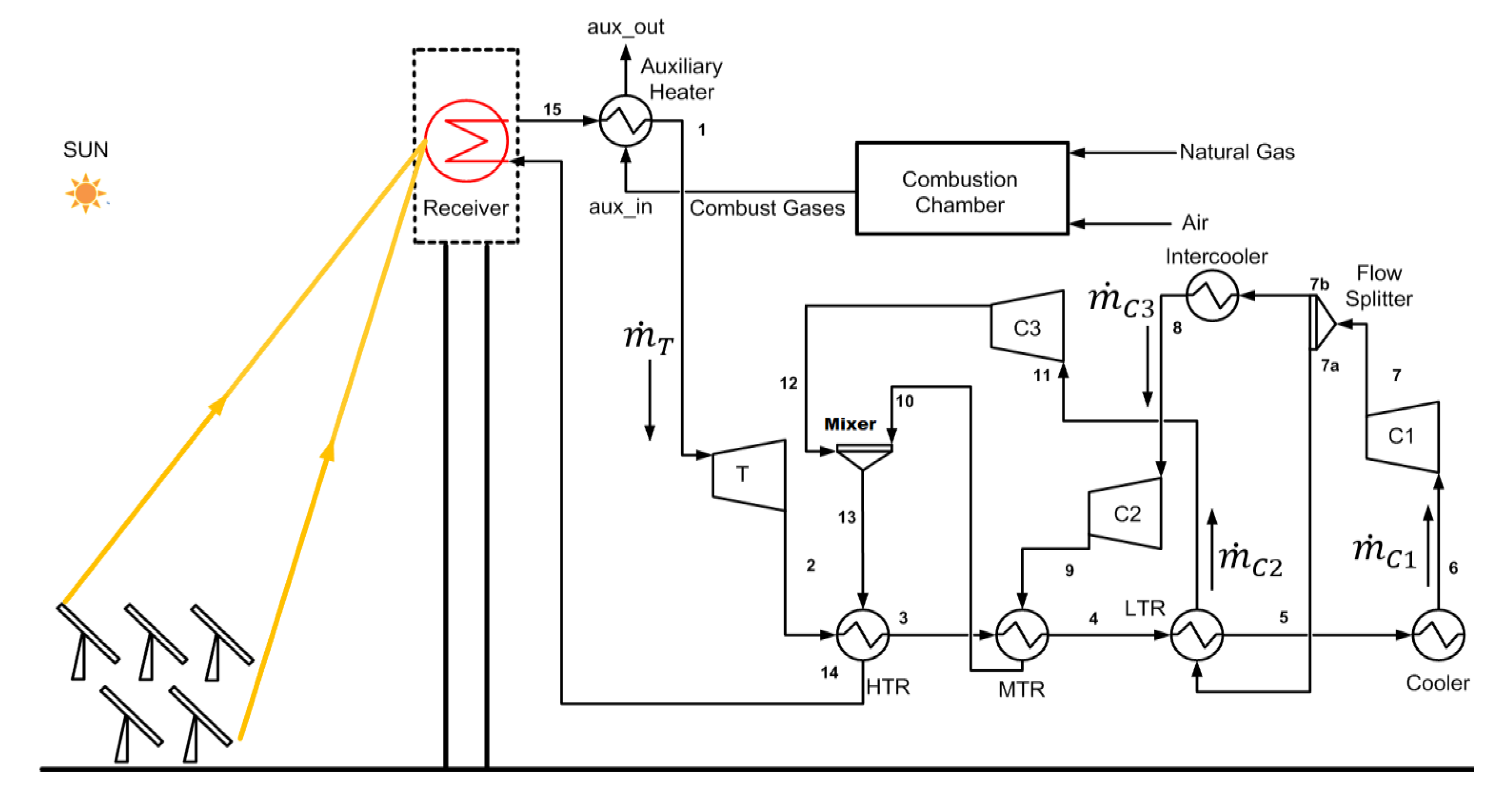
2.1. System Configuration and Key Concepts

This section highlights the basic structure of the work presented in the article. Energy and exergy assessment of S-CO2 Brayton cycle, powered by solar energy, is presented. The recently proposed layout of S-CO2 Brayton cycle by the authors is considered, i.e., recompression Brayton cycle with partial cooling and improved heat recovery (RBC-PC-IHR) [29]. The configuration of the cycle is shown in Figure 1. The stream leaving the low temperature recuperator, LTR, (state 5) is cooled (state 6) and compressed (state 7) in the first stage of the main compressor (C1). The stream leaving the compressor is divided into two parts: one stream (stream 7b) is cooled (state 8) and compressed (state 9) to the cycle’s high pressure, and then flows to a medium temperature recuperator (MTR) to recover the heat; whereas the other stream (stream 7a) recovers heat in LTR (state 11) prior to compression to the cycle’s high pressure in compressor C3. Streams leaving compressor C2 (state 12) and MTR (state 10) are mixed and move to high temperature recuperator, HTR, to recover the heat prior to heating through the solar central heater (receiver). The receiver, sitting on the top of a tower, receives solar energy reflected by the heliostat field. The heat input to the cycle from the receiver varies due to variation in the incident solar energy throughout the day. Therefore, an auxiliary heater, powered by a combustion chamber, is added to maintain a constant heat input to the cycle.
The work presented in the first part of the article deals with the mathematical model to generate a preliminary heliostat field in a radially staggered configuration. The generated field was assessed for its optical efficiency, heat collection rate by the receiver and associated parameters. Monthly averaged heat input to the receiver from the field is computed. The second part deals with the simulation of the power cycle, RBC-PC-IHR, which was simulated in commercial software, Aspen HYSYS V9 (Aspen Technology, Inc., Bedford, MA, USA). Finally, the detailed analysis was conducted to assess the energetic and exergetic performance of the system.

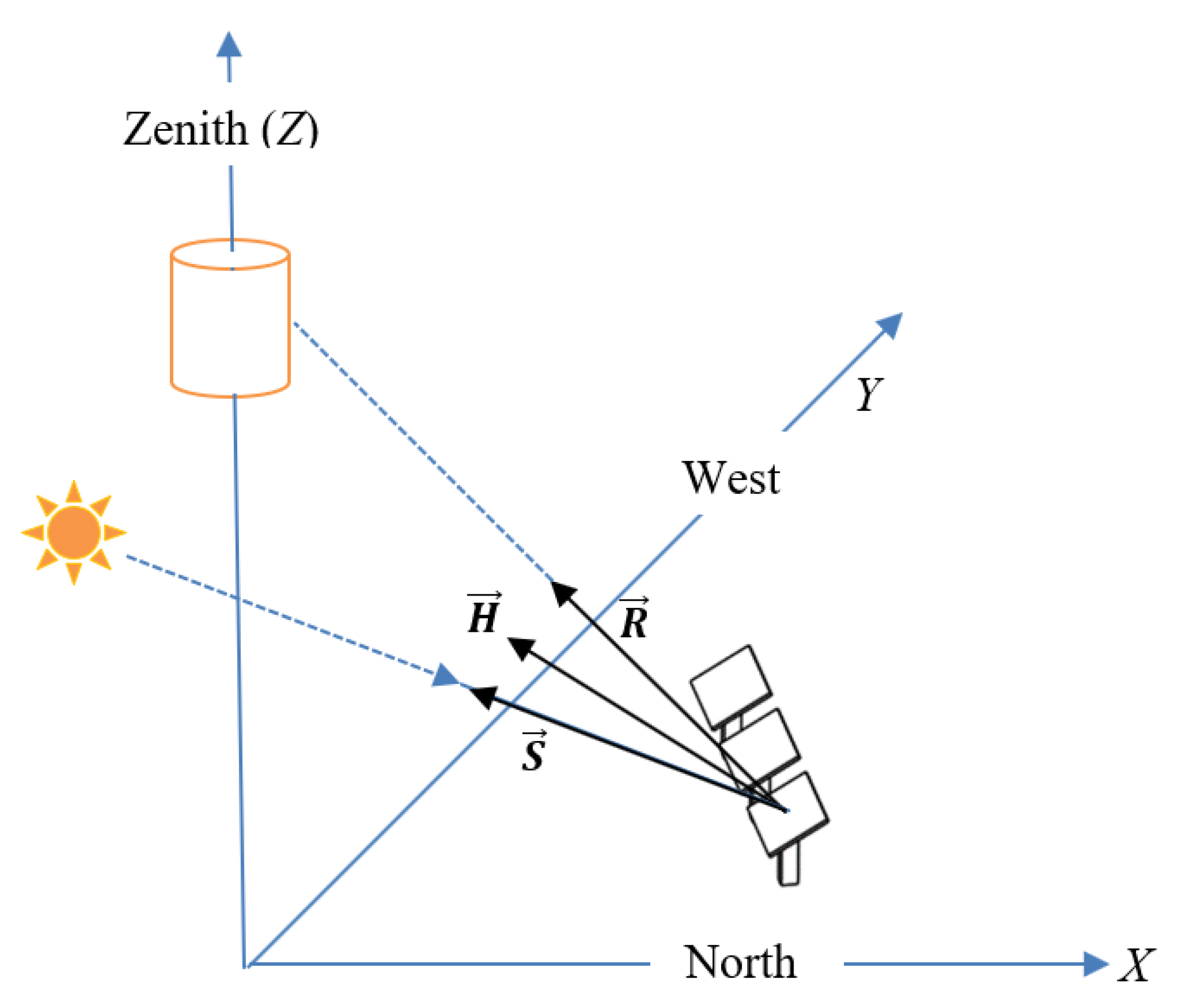
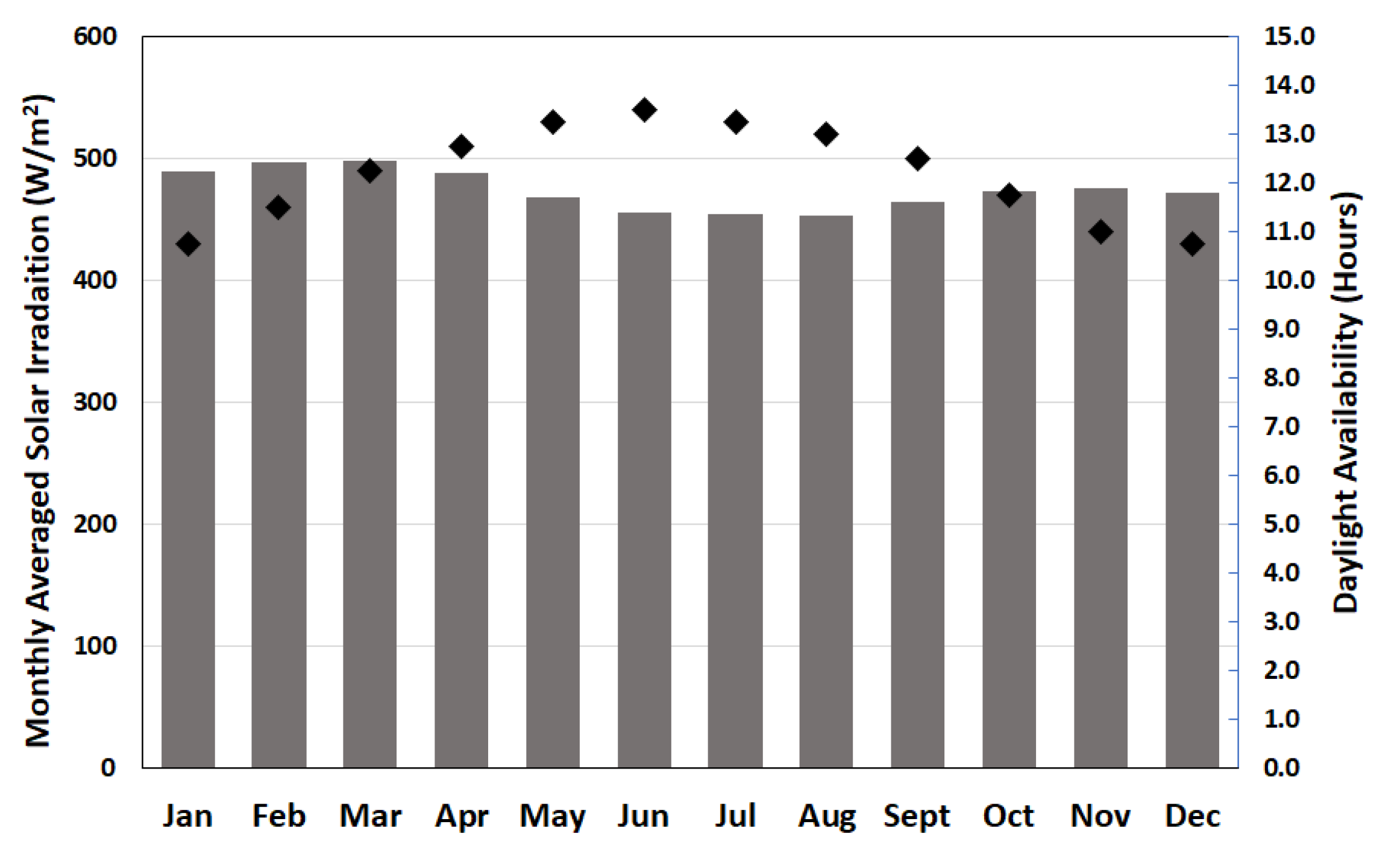
2.2. Solar Radiation Model

ASHRAE clear-sky model was used to calculate the solar insolation level for any given instant [39]. The model predicts the solar intensity received by a surface of unit area placed normal to sun rays, and is given by:
D N I = Ae [ ( e 0.0001148 ( Z ) ) ( B sin α ) ]
where DNI denotes direct solar radiation in W/m2. Z represents the altitude of the location of interest. A and B are solar parameters for apparent solar irradiation beyond the atmosphere and atmospheric extinction coefficient, respectively. Their values are provided by ASHRAE only for the 21st day of each month, as shown in Table 1. Therefore, linear interpolation was used to obtain values for the other days.
The variable α in Equation (1) represents the solar altitude angle and can be calculated from [40]:
sin α = sin l sin δ + cos l c o s δ cos H
where l is the latitude of the location of interest, δ is the declination angle of the sun and H is the hour angle. Variables δ and H are calculated via the following equations [40]:
δ = 23.45 sin [ ( 284 + N ) 360 365 ]
where N is the day number with counting starting from 1 January and ending on 31 December, i.e., 1 N 365 . H is the angular measurement of the local solar time (LST) and is given by following set of equations [40]:
H = ( 12 L S T ) ( 15 o )
L S T = Local   Standard   Time ( L L L S ) ( 4 min deg W ) + E O T
E O T = 9.87 sin ( 2 B N ) 7.53 cos B N 1.5 sin B N
B N = 360 ( N 81 ) / 365
where L S is the standard meridian of local time zone and L L is the longitude of the location of interest. E O T is the equation of time. Direct solar irradiation ( G D ) falling on a surface of any arbitrary orientation can be calculated as
G D = ( D N I ) ( cos θ )
where θ is the angle of incidence between sun rays and the normal to the surface.

2.3. Heliostat Positioning Model

To reflect the solar incident radiation on heliostat to receiver, the heliostat position is controlled by its characteristic angles (tilt angle, β , and surface azimuthal angle, ϕ H ). These angles can essentially be obtained using basic laws of reflection; i.e., the angles of incidence and reflection are equal and the incident ray, the reflected ray and the reflector (heliostat) unit normal lie in the same plane. Based on the basic unit vectors shown in Figure 2 and following basic laws of reflection, we may write
R × H = H × S
where H represents the heliostat surface normal vector. R and S are unit vectors directing receiver and sun from the heliostat, respectively. Thus, the heliostat tilt angle ( β ) and surface azimuthal angle ( ϕ H ) can be calculated using unit normal vector H .
The Cartesian components of unit vector S depend on the latitude l of the location, the solar hour angle h , and the declination angle δ [41].
S x = cos h sin l cos δ + cos l sin δ
S y = sin h cos δ
S z = cos h cos l cos δ + sin l sin δ
The components of the vector representing the relative position of a heliostat with respect to the receiver, R , can be described as
R x = ( X R X H ( X R X H ) 2 + ( Y R Y H ) 2 + ( Z R Z H ) 2 )
R y = ( Y R Y H ( X R X H ) 2 + ( Y R Y H ) 2 + ( Z R Z H ) 2 )
R z = ( Z R Z H ( X R X H ) 2 + ( Y R Y H ) 2 + ( Z R Z H ) 2 )
where X , Y , and Z denote the coordinates of the midpoint of the receiver and the heliostat, respectively, whereas, subscript R is for the reflector and H is for the heliostat. The vector components of H can be obtained using Equation (9):
H x = ( | S z + R z | ( S x + R x ) 2 + ( S y + R y ) 2 + ( S z + R z ) 2 ) ( S x + R x ( S z + R z ) )
H y = ( | S z + R z | ( S x + R x ) 2 + ( S y + R y ) 2 + ( S z + R z ) 2 ) ( S y + R y ( S z + R z ) )
H z = | S z + R z | ( S x + R x ) 2 + ( S y + R y ) 2 + ( S z + R z ) 2
Using vector algebra, the heliostat tilt angle can easily be obtained from
β = cos 1 H z
The heliostat azimuthal angle is defined with reference to south with clockwise measurements considered positive, thus it is defined as:
ϕ H = { π tan 1 | H y H x |                                       if       ( H x > 0   |   H y 0 ) tan 1 | H y H x |                                       if       ( H x 0   |   H y > 0 ) tan 1 | H y H x |                                       if       ( H x < 0   |   H y 0 ) π + tan 1 | H y H x |                                       if       ( H x 0   |   H y < 0 )
Finally, the incidence angle of sun rays on the heliostat using vector algebra with
θ = cos 1 ( H . S )

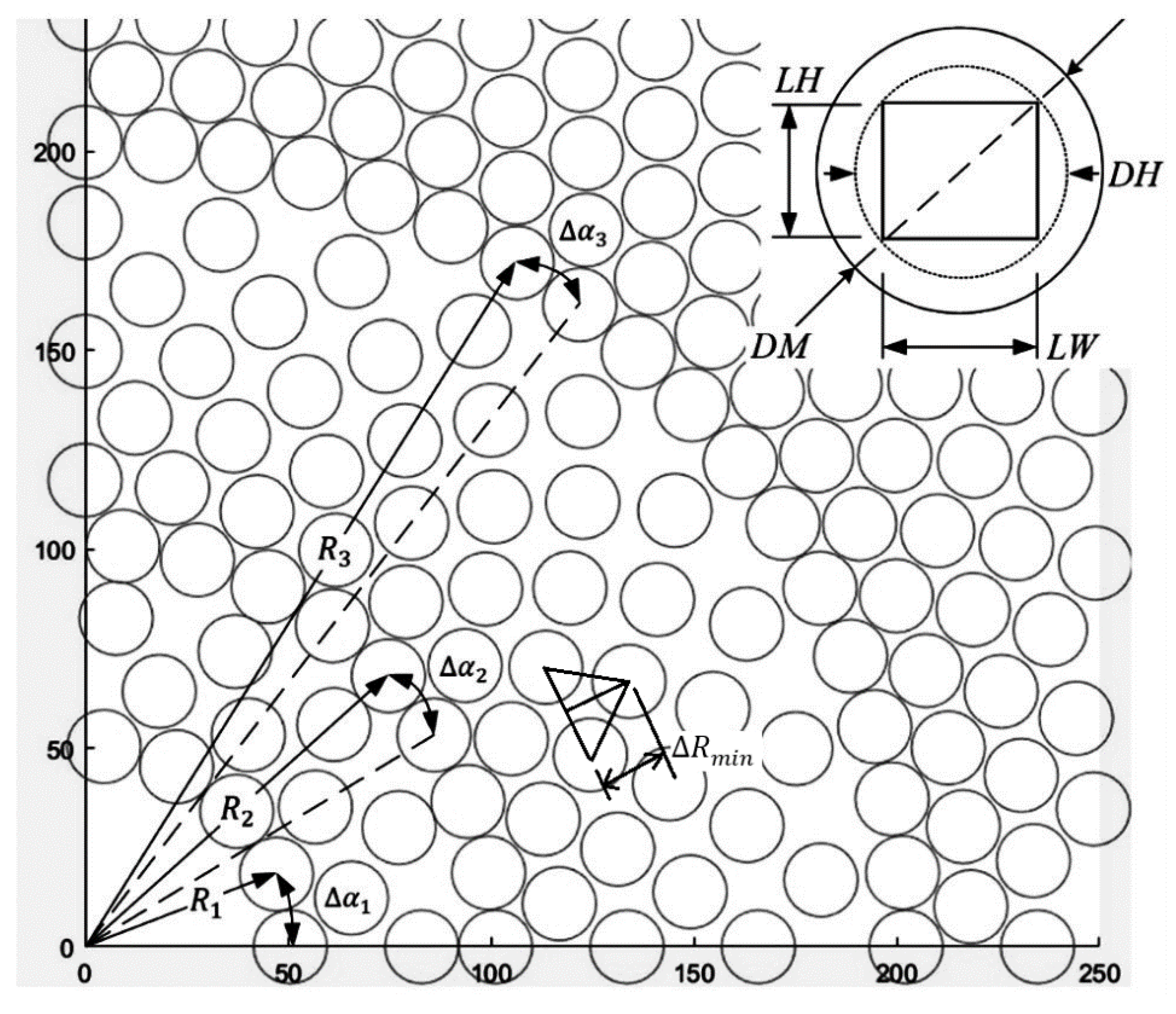
2.4. Heliostat Field Generation

This section describes the model equations and its deployment to the generation of the heliostat field. A radially staggered heliostat field layout was selected for this study due to its simplicity and availability of validated models in the literature. In this layout, heliostats are spread in radially staggered fashion surrounding the solar receiver tower. Refer to Figure 3 for the description of essential variables.
The characteristic diameter DH of a heliostat with an imaginary diameter of a circle enclosing heliostat and is defined as:
D H = 1 + ( L W / L H ) 2 × L H
where L W and L H   denote the width and height of the heliostat, respectively. The characteristic diameter used for the generation of field layout is generally slightly larger than D H ; this allows extra security space between adjacent heliostats and is defined as follows:
D M = ( 1 + ( L W L H ) 2 + d s ) × L H
or
D M = D H + d s e p
where d s e p = d s × L H , represents the extra security spacing. The minimum radial spacing between the staggered heliostat Δ R m i n is a function of D M and can be defined as:
Δ R m i n = D M cos 30 o
The azimuthal spacing Δ α is defined following Collado and Guallar [11]. This represents an angular spacing between adjacent heliostat and is fixed for a given zone of heliostat field. A zone is composed of several rows of heliostat with equal azimuthal spacing. For the first zone, it is defined as:
Δ α 1 = 2   sin 1 ( D M / 2 R 1 ) D M / R 1
where Δ α 1 is the angular spacing for zone 1, R 1 is the radial distance of the first row from the receiver tower. It is obvious that increasing row number will increase the angular distance between the heliostats and when this distance is large enough to accommodate additional heliostats, a new zone is defined with reduced angular distance:
Δ α i =   Δ α i 1 / 2
where subscript i represents the zone number, starting from i = 2 .
The number of rows in each zone is calculated following Collado [11] as:
N r o w s i = R i + 1 R i Δ R m i n round ( 2 i 1   R 1 Δ R m i n )
where subscript i represents the zone number, starting from i = 1 . N r o w s i represents the total number of rows in the ith zone. As the row number is an integer number, the quotients are rounded off.
The number of heliostats in each row of zone 1 or the radius of the first row of zone 1, R 1 , are obtained as [11]:
N h e l 1 = 2 π Δ α 1 = 2 π R 1 D M   R 1 = N h e l 1 × D M 2 π
where N h e l 1 is the number of heliostats in each row of zone 1. It should be noted that R 1 may be controlled by fixing N h e l 1 and D M ; thus, once R 1 is fixed, the number of heliostats for each row in rest of the zones is obtained as:
N h e l i = 2 i π R 1 DM
where N h e l i represents the number of heliostats in each row of the i t h zone. This equation is valid for i = 2 or above.
Starting radii of the first row for the rest of the zones are defined as [42]:
R i = max ( ( 2 R i 1 ) ,   ( R i 1 + ( N r o w s i 1 1 ) Δ R m i n + Δ R m i n ) )
where signifies the zone number, starting from i = 2 .

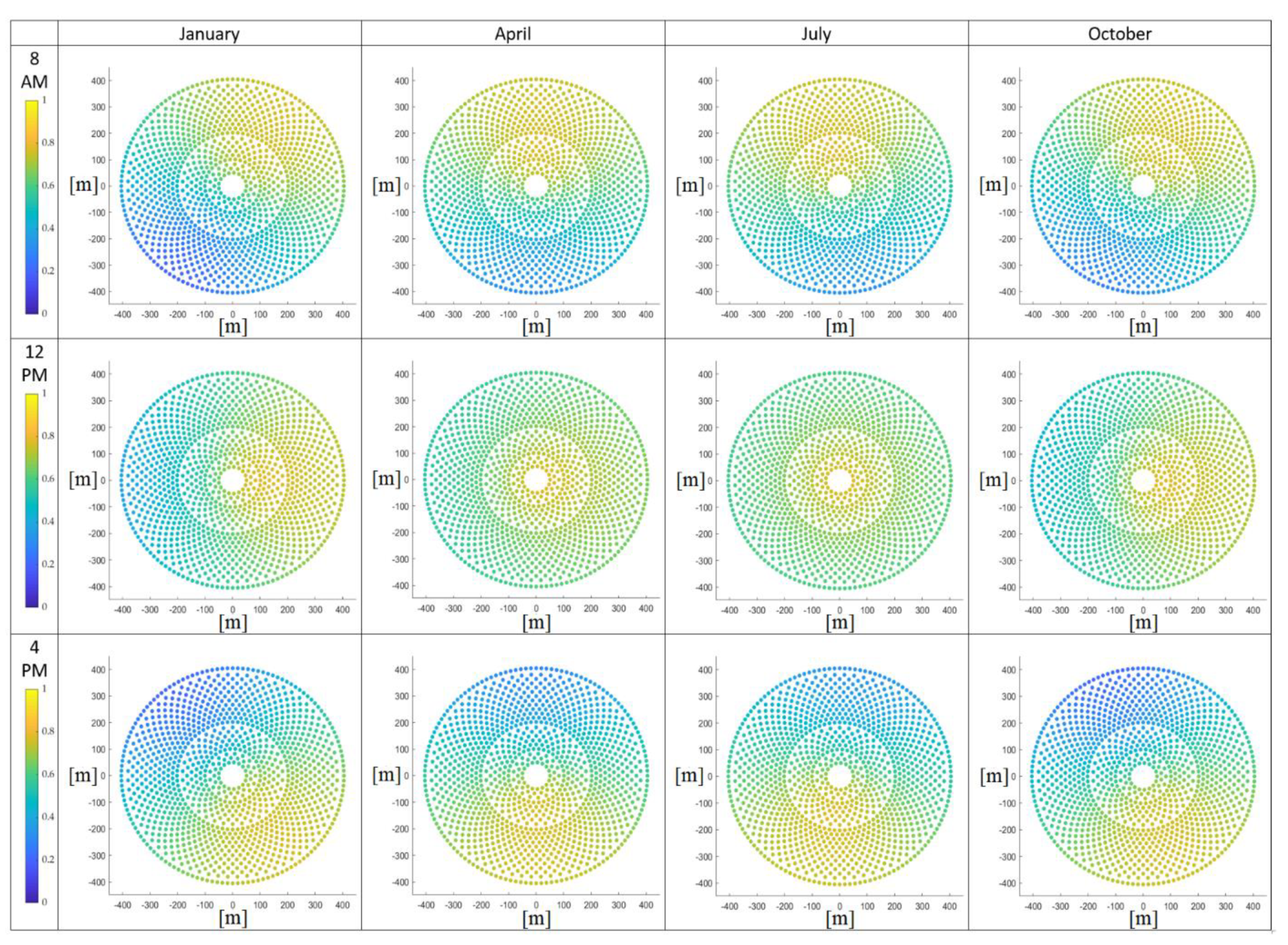
2.4.1. Optical Efficiency of the Heliostat Field

Optical efficiency of the heliostat field represents the fraction of net power absorbed by the receiver to the net power incident on the field. The instantaneous optical efficiency of a heliostat can be described as
η o p t ( X H , Y H , t ) = ρ cos θ ( X H , Y H , t ) f a t ( X H , Y H ) f s b ( X H , Y H , t ) f i t c ( X H , Y H , t )
where η o p t ( X H , Y H , t ) is the instantaneous optical efficiency of a heliostat in the field placed at ( X H , Y H ). The variable ρ is the reflectivity of the heliostat surface; θ ( X H , Y H , t ) , f s b ( X H , Y H , t ) and f i t c ( X H , Y H , t ) represent instantaneous solar incidence angle, blocking and shadowing factor and intercept factor associated with a heliostat located at ( X H , Y H ) on the ground. Blocking and shadowing factor accounts for the percentage of sun rays blocked and not reaching the heliostat and the percentage of reflected rays blocked not reaching the receiver because of adjacent heliostats; this factor is not calculated in the current study; however, for a heliostat field layout its values are between 0.94 and 0.95 (annual average) [10,43]. The variable f a t ( X H , Y H ) is the attenuation factor accounting for the amount of reflected energy scattered and absorbed by the atmosphere before it reaches the receiver and is described as [44,45]:
f a t ( X H , Y H ) = 0.99321 0.0001176 S r e c + 1.97 × 10 8 S r e c 2
if   S r e c 1 km
else
f a t ( X H , Y H ) = exp ( 0.0001106 S r e c )
where S r e c is the slant distance between receiver and a heliostat and can be calculated using Pythagoras theorem as
S r e c = ( X R X H ) 2 + ( Z R Z H ) 2
The intercept factor f i t c ( X H , Y H , t ) in Equation (32) is a significant parameter that describes the fraction of reflected rays intercepted or received by the receiver. In general, reflected rays diverge as they travel away from heliostat, thus increasing the distance between the heliostat and receiver increases the scattering of rays, which results in the leakage of energy flux at the receiver. The HFLCAL model [46] is used to estimate this parameter; this assumes that the reflected energy flux is distributed normally in a circle of radius r with center at the middle of the receiver’s plane, and is given as
f i t c ( X H ,   Y H ,   t ) = 1 2 π σ t o t 2 x R y R exp ( x R 2 + y R 2 2 σ t o t 2 ) d y R d x R
where the integrand represents the normal distribution of energy flux on the receivers’ plane x R and y R are coordinates on the receiver plane. The variable σ t o t is the standard deviation of the normal distribution and is given as [42]
σ t o t = S r e c 2 ( σ s u n 2 + σ b q 2 + σ a s t 2 + σ t 2 )
where σ b q , σ s u n , and σ t are error factors for the quality of beam, the sun shape, the tracking, respectively; σ s u n , σ b q and σ t are assumed to be equal to the same constant values used in [42].
The standard deviation of stigmatic effect is calculated as [46]:
σ a s t = 0.5 ( H t 2 + W s 2 ) 4 S r e c
where H t and W s are image dimensions defined as:
H t = d | S r e c f cos θ |
W s = d | S r e c f cos θ 1 |
where is the focal distance of the heliostat and is equal to S r e c , and d is the characteristic dimension of the heliostat and is given as [47]:
d = L W × L H
where L W and L H are heliostat width and height, respectively. Finally, the instantaneous solar power ( Q ˙ r e c ) absorbed by the central receiver can be calculated as:
Q ˙ r e c = α R   × D N I × N h e l × A H × ( j = 1 j = N h e l η o p t ( X H j , Y H j , t ) )
where N h e l represents total number of heliostats in the field, A H is the area of a heliostat α R is the absorptivity of the receiver material, and D N I denotes instantaneous direct normal irradiation calculated using Equation (1).

2.4.2. Central Receiver and Heat Losses

Radiative heat losses are estimated using model given by Sheu and Mitsos [48] as:
Q ˙ r a d = F v i e w A R ϵ σ T R 4
where F v i e w is the radiation shape factor (considered equal to one), A R is the surface area of the receiver, ϵ is the emissivity of the receiver, σ is the Stefan–Boltzmann constant and T R is the surface temperature of the receiver.
Convective heat losses are calculated using Newton’s law of cooling as:
Q ˙ c o n v = A R h c o n v ( T R T a m b )
where h c o n v is convective heat transfer coefficient. It is estimated using the Bejan correlation for a vertical chamber with natural convection [49] as:
h c o n v = 0.557   × 10 6 ( T R T a m b L R ) 1 / 4   [ kW / m 2 - K ]
where L R is the receiver size (vertical height) and T a m b is the ambient temperature of the environment. Receiver temperature T R is assumed equal to the temperature of S-CO2 at the receiver’s outlet.

2.5. Energy and Exergy Performance Assessments

The authors have previously discussed various configurations and thermodynamic performances of S-CO2 Brayton cycles [29,35,50]. In the current study, recompression Brayton cycle with partial cooling and improved heat recovery is selected due to it simple configuration with high thermodynamic performance. The cycle configuration is shown in Figure 1 with all the necessary state points required to describe the following mathematical models.

2.5.1. Energy Model

The thermal efficiency of the cycle is calculated as:
η t h = ( W ˙ T   W ˙ C 1 W ˙ C 2 W ˙ C 3 ) / ( Q ˙ s o l i n + Q ˙ a u x i n )
Here, W ˙ T is the turbine power output, W ˙ C 1 , W ˙ C 2 and W ˙ C 3 represent power consumed by compressors C1, C2 and C3, respectively. Q ˙ s o l _ i n is the solar power input to the cycle and is defined as:
Q ˙ s o l i n = Q ˙ r e c Q ˙ r a d Q ˙ c o n v
Q ˙ a u x _ i n is the additional power input from an auxiliary heater, required to maintain a constant net power output of the cycle, and is defined as:
Q ˙ a u x _ i n = m ˙ a u x ( h a u x i n   h a u x o u t ) = m ˙ T ( h 1 h 15 )
The power associated with turbine and compressors can be defined as:
W ˙ T = m ˙ T ( h 1 h 2 )
W ˙ C 1 = m ˙ C 1 ( h 7 h 6 )    
W ˙ C 2 = m ˙ C 2 ( h 9 h 8 )    
W ˙ C 3 = m ˙ C 3 ( h 12 h 11 )    
Heat exchanger effectiveness is defined for the total hot stream as [51,52]:
ϵ h o t ,   s t r e a m = ( h 2 h 5 ) / ( h 2 h 5 @ ( T 7 , P 5 ) )
where h 5 @ ( T 7 , P 5 ) is the enthalpy of the hot stream at the outlet of LTR calculated based on the minimum temperature that it could achieve [53].
For the solar driven thermal power plant integrated with an auxiliary heater, the degree of fuel hybridization can be defined as:
f h y b r i d = ( Q ˙ a u x i n ) / ( Q ˙ s o l i n + Q ˙ a u x i n )

2.5.2. Exergy Model

Exergy represents the energy that is available in the system to be used. It becomes zero when system attains equilibrium with its surroundings. The exergy analysis is done to quantify the thermodynamic imperfection of the process under consideration. This section provides details of exergy modeling of the complete system.
The total solar exergy input to the heliostat field is defined following Petela [54]:
ψ ˙ s o l a r = D N I   × N h e l × A H × ( 1 + 1 3 ( T r e f T s u n ) 4 4 3 ( T r e f T s u n ) )
where T s u n is the surface temperature of sun’s outer layer and is taken as 5800 K [54], whereas, T r e f is the reference temperature, which is the ambient temperature of the surroundings and is considered equal to 298 K.
The net exergy input to the central receiver can be defined as:
ψ ˙ r e c = Q ˙ r e c ( 1 T r e f T R )
Thus, the amount of exergy loss in the heliostat field can be calculated as:
ψ ˙ l o s s ,   h e l i o s t a t = ψ ˙ s o l a r ψ ˙ r e c
The amount of useful exergy gain by the central receiver is calculated as:
ψ ˙ r e c ,   u s e f u l = Q ˙ s o l i n ( 1 T r e f T R )
For the Brayton cycle, the exergy at any state   k is calculated as:
ψ ˙ k = m ˙ k ( h k T r e f s k )
The exergy loss in the central receiver is then calculated as:
ψ ˙ l o s s , r e c = ψ ˙ r e c , u s e f u l ( ψ ˙ 15 ψ ˙ 14 )
The exergy input to CO2 in the auxiliary heater is equal to the difference of exergies of combustion gases at the inlet and the outlet the auxiliary heater and is calculated as:
ψ ˙ a u x = ψ ˙ a u x i n ψ ˙ a u x o u t
The net exergy input to the Brayton cycle is then defined as:
ψ ˙ i n p u t , B C = ψ ˙ r e c ,   u s e f u l + ψ ˙ a u x
The exergy loss (irreversibility) in the remaining components of the plant is calculated according to following equations:
ψ ˙ l o s s ,   T = ( ψ ˙ 1 ψ ˙ 2 ) W ˙ T
ψ ˙ l o s s ,   C 1 = W ˙ C 1 ( ψ ˙ 7 ψ ˙ 6 )
ψ ˙ l o s s ,   C 2 = W ˙ C 2 ( ψ ˙ 9 ψ ˙ 8 )
ψ ˙ l o s s ,   C 3 = W ˙ C 3 ( ψ ˙ 12 ψ ˙ 11 )
ψ ˙ l o s s ,   H T R = ( ψ ˙ 2 ψ ˙ 3 ) ( ψ ˙ 14 ψ ˙ 13 )
ψ ˙ l o s s ,   M T R = ( ψ ˙ 3 ψ ˙ 4 ) ( ψ ˙ 10 ψ ˙ 9 )
ψ ˙ l o s s ,   L T R = ( ψ ˙ 4 ψ ˙ 5 ) ( ψ ˙ 11 ψ ˙ 7 a )
ψ ˙ l o s s ,   a u x = ( ψ ˙ a u x i n ψ ˙ a u x o u t ) ( ψ ˙ 1 ψ ˙ 15 )
The cooler and intercooler are air cooled; therefore, a portion of exergy input to coolers is transferred to cooling air as a result of heat transfer. The exergy gain by the cooling air in each cooler can be approximated as [51]:
ψ ˙ g a i n , a i r = m ˙ a i r [ ( h o u t h i n ) T r e f ( s o u t s i n ) ] a i r
The amount of exergy loses by carbon dioxide in each cooler can be calculated as [51]:
ψ ˙ l o s s , C O 2 = m ˙ C O 2 [ ( h i n h o u t ) T r e f ( s i n s o u t ) ] C O 2 ψ ˙ g a i n , a i r
The net exergy loss in both coolers is equal to exergy loss by the carbon dioxide in each cooler plus exergy gain by the air from each cooler. This can be calculated as:
ψ ˙ l o s s , c o o l e r = ( ψ ˙ g a i n , a i r ) C o o l e r + ( ψ ˙ g a i n , a i r ) I n t e r c o o l e r   +   ( ψ ˙ l o s s , C O 2 ) C o o l e r +   ( ψ ˙ l o s s , C O 2 ) I n t e r c o o l e r

2.6. Operating Parameters and Simulation Environment

2.6.1. Solar Radiation, Heliostat Field and Receiver

The mathematical model for solar radiation, heliostat field and receiver discussed in the previous section, from Equation (1) to Equation (45), was simulated using a suite of codes developed in MATLAB. A set of subroutines were developed to generate a radially staggered field, which was called in the main program for calculating instantaneous characteristic angles of the heliostats such that it reflects the incoming solar beam to the central receiver. Riyadh city (24.7136° N, 46.6753° E) in Saudi Arabia is considered as a location of interest to perform thermodynamic analysis of a solar driven power plant. Table 2 presents basic design parameters for the heliostat field and receiver.

2.6.2. S-CO2 Brayton Cycle

S-CO2 Brayton cycle, RBC-PC-IHR, was simulated in the commercial software Aspen HYSYS V9 (Aspen Technology, Inc., Bedford, MA, USA) using the Peng–Robinson model for state property calculations. The analysis was done with the following assumptions [7,27,29,51,57,58]:
  • The cycle operates under steady-state conditions with no pressure drop in the pipelines and heat exchangers.
  • The turbine and compressor isentropic efficiencies are 93% and 89%, respectively.
  • The heat exchanger effectiveness is 95% with a minimum pinch point temperature ( Δ T min )   of 5 °C.
  • Cooler and intercooler are dry cooled with air as coolant. Energy needed to operate air coolers is neglected.
  • The cycle maximum pressure is 25 MPa.
  • Compressor inlet temperature and pressure are maintained at 40 °C and 7.5 MPa corresponding to state 8.
  • The turbine inlet temperature is 600 °C.
  • Auxiliary heater effectiveness is 90%.
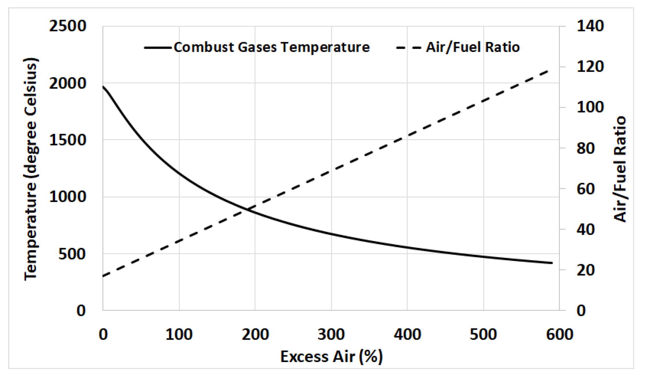
  • The combustion chamber uses methane as a fuel with 300% excess air. This maintains the temperature of combustion gases at approximately at 673 °C.
  • Cycle receives a constant power input of 80 MW.
  • Energy consumed by solar tower auxiliaries is neglected.

3. Results and Discussions

Thermodynamic performance analysis of the power plant was done for daylight hours during which the plant would operate on solar energy and an auxiliary heat source. To assess the optical performance of the heliostat field, the data were generated for each heliostat from sunrise until sunset. The calculations were made for every 15 minutes for each day from 1 January to 31 December. The calculated parameters are solar angles, heliostat characteristic angle, intercept factor, attenuation factor, solar incidence angle, direct normal irradiation and optical efficiency.
The optical efficiency of the heliostat field represents how effectively incident solar energy is directed to the target. Instantaneous field optical efficiency is plotted in Figure 4. For the sake of discussion, plots are shown only for January, April, July and October, at 8 a.m., 12 p.m. and 4 p.m. It is observed that the heliostats placed on the western side of the tower have higher efficiency in the morning, which happens due to a smaller angle of incidence for these heliostats. As the day passes and sun altitude angle increases, the heliostats change their orientation (tilt and surface azimuth angles) such that they reflect the solar beam to the tower and so their optical efficiency varies throughout the day. In the afternoon, the sun is on the western side of the tower; therefore, heliostats placed on the eastern side of the tower have more contribution in overall optical efficiency of the field.
The monthly averaged values of optical efficiency and the intercept factor from sunrise until sunset are calculated and presented in Table 3. The optical efficiency of the field is the lowest in December, which gradually increases and peaks in the month of June; afterward a gradual decline is observed for the rest of the months. The annual average optical efficiency of the heliostat field is nearly 59.14%. The intercept factor is an important parameter that represents the fraction of reflected rays received by the receiver. The monthly averaged values of intercept factors are also shown in Table 3 for each month and its annual average value of around 99%. Figure 5 represents the monthly averaged solar energy incident on the field per unit area of the heliostat from 8 a.m. to 4 p.m. From January to April, the values are slightly higher than rest of the months; however, the annual average direct solar energy received by the heliostat field is approximately 475 W/m2.
Recompression Brayton cycle with partial cooling and improved heat recovery (RBC-PC-IHR) layout was selected to assess the performance of the overall system. The authors recently proposed this layout and reported better thermodynamic performance of RBC-PC-IHR layout over simple Brayton cycle, recompression Brayton cycle and recompression Brayton cycle with partial cooling configurations [29]. The power cycle operates on solar energy and an auxiliary heat source, and receives a constant net thermal power input of 80 MW. The cycle was simulated with a turbine operating temperature of 600 °C and operating pressure adjusted to maintain a minimum pinch temperature of 5 °C. Table 4 shows the energy balance for the power cycle. The thermal efficiency of the cycle is 46.44%; therefore, the cycle’s net shaft power output was approximately 37.15 MW.
The energetic and exergetic performance of the plant was done with solar energy input to the cycle from 8 a.m. to 4 p.m. Thus, the cycle would be operating on solar energy and auxiliary heat source from 8 a.m. to 4 p.m.; afterwards, only the auxiliary heat source would be utilized. Monthly averaged estimate of the availability of solar energy during 8 a.m. to 4 p.m. and the requirement of auxiliary heat is plotted in Figure 6a. The maximum and minimum heat absorbed by the receiver occur in March (84.42 MW) and December (77.2 MW), respectively. However, on annual basis the average solar heat absorbed by the receiver is nearly 79.7 MW. Heat lost by the receiver due to natural convection and radiation is also plotted in Figure 6a. The yearly averaged heat loss from the receiver is 7.8 MW approximately, which corresponds to approximately 10% of that absorbed by the receiver. As the cycle is provided a constant net power input of 80 MW, the auxiliary heat required on a monthly basis is shown in Figure 6a with a minimum 3.77 MW needed in March and maximum 10.5 MW in December. The net solar and auxiliary heat energy input, in MWh, to the cycle from 8 a.m. to 4 p.m. is also plotted in Figure 6b.
The auxiliary heater was operated on hot combustion gases. Methane was used as a fuel in the combustion chamber with an excess air supply of 300%, which maintains the temperature of combustion gases at nearly 675 °C. The effect of excess air on the combustion temperature and air to fuel ratio is plotted in Figure 7. These combustion gases were then used to heat the carbon dioxide to desired turbine inlet temperature of 600 °C. The percentage of fuel hybridization and the mass flow rate of the fuel (methane) needed for steady operation of plant from 8 a.m. to 4 p.m. is plotted in Figure 8. A minimum 0.64 kg/s and a maximum 1.5 kg/s fuel are required in March and December, respectively. It is also observed that from 8 a.m. to 4 p.m. the plant operates on nearly 95% solar energy in March, requiring only 5% of fuel hybridization. On the other hand, nearly 13% fuel hybridization is needed in July and December.
Exergy analysis of the plant is carried out by calculating the exergy losses in each component following Equations (55) to (73). Figure 9a represents the distribution of exergy for the heliostat field and the receiver. The highest solar exergy input to the system is observed for the months of February and March (nearly 131 MW), whereas, the minimum exergy input is 117 MW occurring in July. The yearly averaged exergy input to the heliostat field and the exergy input to the receiver are approximately 123.5 MW and 52.5 MW, thus, nearly 42.5% of the exergy is lost in the heliostat field. A portion of exergy input to the receiver is lost due to natural convection and radiation; the remaining useful exergy input to the power cycle (useful exergy gain by the receiver) is plotted in Figure 9b. Approximately 5 MW of input exergy received by the central receiver is lost due to convection and radiation, which corresponds to nearly 5% loss of the input exergy.
Exergy losses during the heat transfer process to CO2 in the receiver and the auxiliary heater are plotted in Figure 10. On average, 3.22 MW (almost 7.5% of useful exergy gain by the receiver) of exergy loss occurs in the solar central receiver during the heat transfer process, refer to Figure 10a. On the other hand, a significantly small percentage of exergy loss occurs in auxiliary heater (2.3% of exergy input), as seen from Figure 10b. The exergy losses in the auxiliary heater are lower for months with higher solar incident exergy due to lower mass flow rate of fuel required to supplement the solar energy input to the cycle.
Finally, exergy losses occurring in various components of the Brayton cycle are plotted in Figure 11. Considering exergy losses in turbomachines (turbine and compressors), the turbine incurs the highest exergy loss because the maximum temperature of the working fluid in the cycle is at the inlet of the turbine. Among compressors, compressor C1 experiences the highest exergy loss, which is due to the fact that it handles the net mass flow rate of the cycle, whereas, compressors C2 and C3 receive only a portion of net mass flow rate due to the flow splitter. Exergy loss incurred in compressor C3 is higher than the exergy loss that takes place in compressor C2; this is a result of heat recuperation by CO2 in LTR, which increases its temperature before it enters compressor C3. Among heat recuperators, HTR operates at a higher temperature than MTR and LTR. In other words, HTR has a higher difference in the operating conditions from its surrounding state, resulting in the higher exergy loss in comparison to what incurs in MTR and LTR. LTR is operated at much lower temperature than MTR, resulting in the lowest exergy loss. Exergy losses in the cooler and the intercooler, and the exergy gain by the coolant (air) in cooler and intercooler are considered as a net loss in available exergy to the cycle. The cooler handles a higher mass flow rate than the intercooler (because the net mass flow rate of the working fluid in the cycle splits after compressor C1), thus it experiences more exergy loss than the intercooler. Similarly, exergy gain by the air in the cooler is significantly higher than the intercooler due to the same reason. The net exergy loss in the coolers (cooler and intercooler), defined by Equation (73), is nearly 4.4 MW.

4. Conclusions

Energy and exergy performances of a solar thermal power plant were investigated. Recompression Brayton cycle with partial cooling and improved heat recovery (RBC-PC-IHR) configuration was considered, driven mainly by solar energy from 8 a.m. to 4 p.m. Auxiliary heat was supplied to account for the fluctuations in the intensity of solar irradiation. The analysis was conducted for Riyadh (the capital city of Saudi Arabia) and the solar energy was collected from a radially staggered heliostat field. Optical efficiencies of the generated field were calculated. A sun-tracking method was implemented to calculate the characteristic angles of each heliostat in the field and data were generated for every fifteen minutes from sunrise until sunset. Following are the key outcomes and concluding remarks:
  • The average annual optical efficiency of the heliostat field was nearly 59 percent with a capability of providing 475 watts of power per unit heliostat’s area to the central receiver.
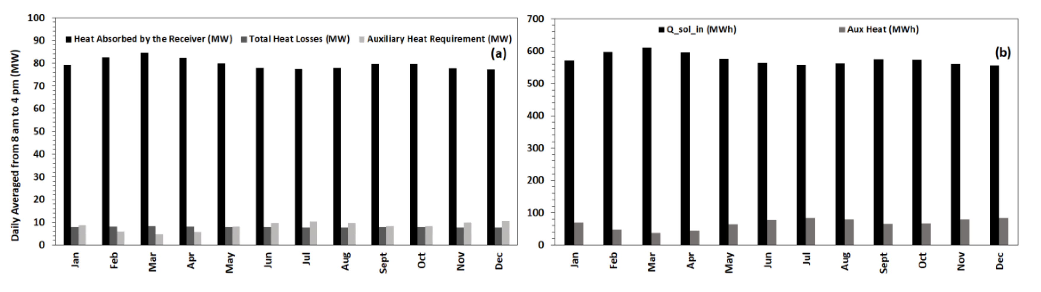
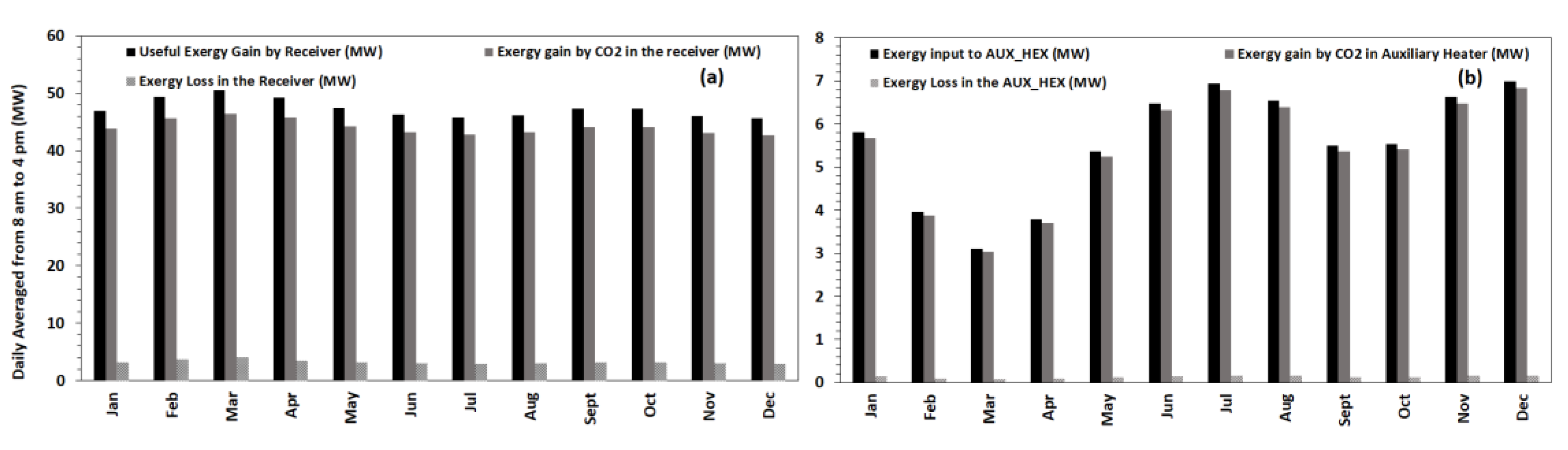
  • The average annual solar heat absorbed by the receiver is approximately 79.7 MW, out of which nearly 10 percent is lost due to natural convection and radiation.
  • The power cycle was operated with a turbine inlet temperature of 600 °C and provided a constant net power input of 80 MW.
  • The auxiliary heater, operating on combustion gases with methane as fuel in the combustion chamber, provided extra heat required for the steady operation of the cycle. The average annual fuel requirement is 1.2 kg/s.
  • On a monthly basis, for the month of March, the plant was found to be least dependent on auxiliary heat and operated 95% on the solar energy, whereas, a maximum of 13% auxiliary heat support was required in December.
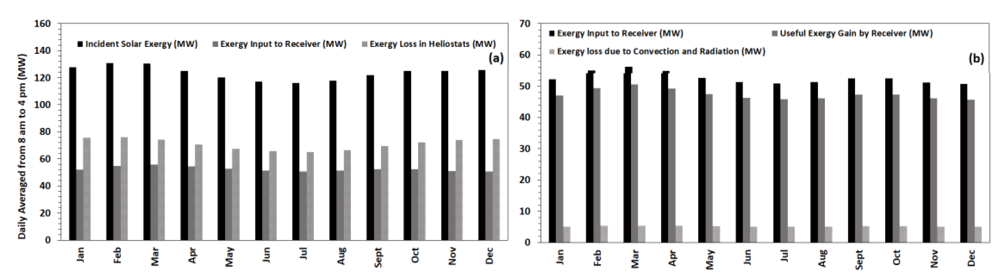
  • Exergy analysis revealed a maximum loss occurs in the heliostat field, which is nearly 42.5% of incident solar exergy.
  • Approximately 5% of exergy absorbed by the central receiver was lost due to natural convection and radiation. Furthermore, the central receiver experienced 7.5% loss in the remaining exergy while transferring heat to the working fluid (carbon dioxide).
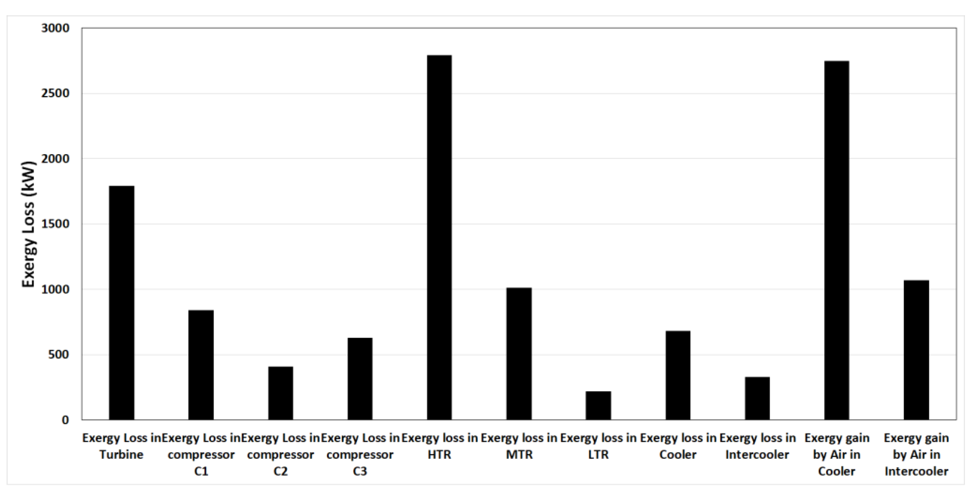
  • Nearly 7.5% of the net exergy received by CO2 from the solar central receiver and the auxiliary heater is lost in turbomachines (turbine and compressors). On the other hand, heat recuperators (LTR, HTR and MTR) and coolers (cooler and intercooler) incurred approximately 8.1% and 10% of net exergy gain by CO2, respectively.

Author Contributions

Conceptualization, M.E.S. and K.H.A.; methodology, M.E.S.; software, M.E.S.; validation, M.E.S. and K.H.A.; formal analysis, M.E.S.; investigation, M.E.S. and K.H.A.; writing—original draft preparation, M.E.S.; writing—review and editing, M.E.S. and K.H.A.; visualization, M.E.S. and K.H.A.; funding acquisition, M.E.S. and K.H.A. All authors have read and agreed to the published version of the manuscript.

Funding

This project was funded by the Deanship of Scientific Research (DSR), King Abdulaziz University, Jeddah, under grant No. D-095-135-1441. The authors, therefore, gratefully acknowledge DSR technical and financial support.

Conflicts of Interest

The authors declare no conflict of interest.

Nomenclature

AApparent solar irradiation beyond the atmosphereW/m2 Q ˙ c o n v Convective heat loss, MW
BAtmospheric extinction coefficient Q ˙ s o l i n Solar power input to the cycle, MW
A H Heliostat surface area, m2 Q ˙ a u x i n Auxiliary power input to the cycle, MW
d Square root of the area of the heliostat, m R 1 Radius of the first ring of the first zone of the heliostat field, m
d s e p Extra security distance, m R x , R y , R z Spatial (x, y, z) components of the unit vector of reflected ray of the sun from heliostat pointing receiver
DRDiameter of the receiver, m S x , S y , S z Spatial (x, y, z) components of the unit vector directing sun ray
D M Characteristic diameter, m S r e c Slant distance between the receiver and the heliostat, m
D H Heliostat diagonal, m s Entropy, kJ/kg
D N I Direct normal irradiation, W/ m2 T R Receiver surface temperature, K
EOTEquation of time T r e f Reference temperature, K
f i t c Intercept factor of the heliostatTHTTower optical height, m
f a t Atmospheric attenuation factor W s image dimension in the sagittal plane, m
f s b Shading and blocking factor W ˙ T Turbine power output, MW
f Focal distance W ˙ C 1 Compressor 1 power consumption, MW
f h y b r i d Degree of hybridization W ˙ C 2 Compressor 2 power consumption, MW
F v i e w Radiation shape factor x R x-coordinate on the receiver plane
G D Direct solar radiation, W/ m2 X R , X H x-coordinates of the receiver and the heliostat
H Hour angle, degree Y R , Y H y-coordinates of the receiver and the heliostat
h Mass enthalpy, kJ/kg y R y-coordinate on the receiver plane
h c o n v Convective heat transfer coefficientZ Altitude of the location, m
H t image dimension in the tangential plane, m Z R , Z H z-coordinates of the receiver and the heliostat
H x , H y , H z Spatial (x, y, z) components of the surface normal unit vector of the heliostat α Solar altitude angle, degree
HTRHigh temperature recuperator α R Absorptivity of the receiver
l Latitude of the location, m δ Sun’s declination angle, degree
LSTLocal solar time, hours θ Solar incidence angle, degree
L S Standard meridian of local time zone ϕ H Heliostat surface azimuth angle, degree
L L Longitude of the location β Heliostat tilt angle, degree
L W Heliostat width, m Δ R m i n Minimum radial spacing between heliostat rows, m
L H Heliostat height, m Δ α i Azimuthal spacing between heliostats in the ith zone of heliostat field, degree
LRLength of the receiver, m η t h Thermal efficiency of the plant
LTRLow temperature recuperator ψ ˙ Exergy, kW or MW
MTRMedium temperature recuperator η o p t Optical efficiency
m ˙ T Mass flow rate in the turbine, kg/s ρ Reflectivity of the heliostat mirror
m ˙ C 1 Mass flow rate in the compressor 1, kg/s ϵ Emissivity of the receiver
m ˙ C 2 Mass flow rate in the compressor 2, kg/s ϵ h o t ,   s t r e a m Heat exchanger effectiveness
m ˙ C 3 Mass flow rate in the compressor 3, kg/s σ Stefan Boltzmann constant
NDay number of the year σ t o t Standard deviation of the normal distribution
N r o w s i Number of rows in the ith zone of heliostat field σ s u n Error factor for the sun shape
N h e l i Number of heliostats in each row of the i t h zone σ b q Error factor for the quality of the beam
Q ˙ r e c Solar power absorbed by receiver, MW σ a s t Error factor for the stigmatic effect
Q ˙ r a d Radiative heat loss, MW σ t Error factor for the tracking

References

  1. Pfahl, A. Survey of Heliostat Concepts for Cost Reduction. J. Sol. Energy Eng. 2013, 136, 014501. [Google Scholar] [CrossRef]
  2. Steinmann, W.-D. Thermal energy storage systems for concentrating solar power (CSP) technology. In Advances in Thermal Energy Storage Systems; Elsevier: Amsterdam, The Netherlands, 2015; pp. 511–531. [Google Scholar]
  3. Xu, B.; Li, P.; Chan, C.; Tumilowicz, E. General volume sizing strategy for thermal storage system using phase change material for concentrated solar thermal power plant. Appl. Energy 2015, 140, 256–268. [Google Scholar] [CrossRef] [Green Version]
  4. Islam, K.; Hosenuzzaman, M.; Rahman, M.; Hasanuzzaman, M.; Rahim, N.A. Thermal performance improvement of solar thermal power generation. In Proceedings of the 2013 IEEE Conference on Clean Energy and Technology (CEAT), Lankgkawi, Malaysia, 18–20 November 2013; pp. 158–162. [Google Scholar]
  5. Zhai, R.; Zhao, M.; Li, C.; Peng, P.; Yang, Y. Improved Optimization Study of Integration Strategies in Solar Aided Coal-Fired Power Generation System. Int. J. Photoenergy 2015, 2015, 1–8. [Google Scholar] [CrossRef] [Green Version]
  6. Praveen, P.R. Performance Analysis and Optimization of Central Receiver Solar Thermal Power Plants for Utility Scale Power Generation. Sustainability 2019, 12, 127. [Google Scholar]
  7. Atif, M.; Al-Sulaiman, F.A. Energy and exergy analyses of solar tower power plant driven supercritical carbon dioxide recompression cycles for six different locations. Renew. Sustain. Energy Rev. 2017, 68, 153–167. [Google Scholar] [CrossRef]
  8. Han, Y.; Xu, C.; Xu, G.; Zhang, Y.; Yang, Y. An Improved Flexible Solar Thermal Energy Integration Process for Enhancing the Coal-Based Energy Efficiency and NOx Removal Effectiveness in Coal-Fired Power Plants under Different Load Conditions. Energies 2017, 10, 1485. [Google Scholar] [CrossRef] [Green Version]
  9. Noone, C.J.; Torrilhon, M.; Mitsos, A. Heliostat field optimization: A new computationally efficient model and biomimetic layout. Sol. Energy 2012, 86, 792–803. [Google Scholar] [CrossRef]
  10. Besarati, S.M.; Goswami, D. A computationally efficient method for the design of the heliostat field for solar power tower plant. Renew. Energy 2014, 69, 226–232. [Google Scholar] [CrossRef]
  11. Collado, F.J.; Guallar, J. Campo: Generation of regular heliostat fields. Renew. Energy 2012, 46, 49–59. [Google Scholar] [CrossRef]
  12. Collado, F.J.; Guallar, J. Fast and reliable flux map on cylindrical receivers. Sol. Energy 2018, 169, 556–564. [Google Scholar] [CrossRef]
  13. Cruz, N.; Redondo, J.L.; Berenguel, M.; Álvarez, J.; Ortigosa, P.; Álvarez, J.D. Review of software for optical analyzing and optimizing heliostat fields. Renew. Sustain. Energy Rev. 2017, 72, 1001–1018. [Google Scholar] [CrossRef]
  14. Feher, E. The supercritical thermodynamic power cycle. Energy Convers. 1968, 8, 85–90. [Google Scholar] [CrossRef]
  15. Angelino, G. Carbon Dioxide Condensation Cycles for Power Production. J. Eng. Power 1968, 90, 287–295. [Google Scholar] [CrossRef]
  16. Dostál, V.; Driscoll, M.J.; Hejzlar, P. A Supercritical Carbon Dioxide Cycle for Next Generation Nuclear Reactors. Tech. Rep. MIT-ANP-TR-100; Massachusetts Institute of Technology: Cambridge, MA, USA, 2004; pp. 1–137. [Google Scholar]
  17. Angelino, G. Real Gas Effects in Carbon Dioxide Cycles. In Proceedings of the ASME 1969 Gas Turbine Conference and Products Show, Cleveland, OH, USA, 9–13 March 1969. [Google Scholar]
  18. Turchi, C.S.; Ma, Z.; Dyreby, J. Supercritical Carbon Dioxide Power Cycle Configurations for Use in Concentrating Solar Power Systems. In Proceedings of the ASME Turbo Expo 2012: Turbine Technical Conference and Exposition, Copenhagen, Denmark, 11–15 June 2012; pp. 967–973. [Google Scholar]
  19. Ahn, Y.; Bae, S.J.; Kim, M.; Cho, S.K.; Baik, S.; Lee, J.I.; Cha, J.E. Review of supercritical CO2 power cycle technology and current status of research and development. Nucl. Eng. Technol. 2015, 47, 647–661. [Google Scholar] [CrossRef] [Green Version]
  20. Chen, Y.; Lundqvist, P.; Johansson, A.; Platell, P. A comparative study of the carbon dioxide transcritical power cycle compared with an organic rankine cycle with R123 as working fluid in waste heat recovery. Appl. Therm. Eng. 2006, 26, 2142–2147. [Google Scholar] [CrossRef]
  21. Vesely, L.; Dostal, V.; Hajek, P. Design of Experimental Loop with Supercritical Carbon Dioxide. In Proceedings of the 22nd International Conference on Nuclear Engineering, Prague, Czech Republic, 7–11 July 2014. [Google Scholar]
  22. Turchi, C.S. Supercritical CO2 for Application in Concentrating Solar Power Systems. In Proceedings of the supercritical CO2 Power Cycle Symposium, Troy, NY, USA, 29–30 April 2009. [Google Scholar]
  23. Wang, X.; Dai, Y. Exergoeconomic analysis of utilizing the transcritical CO2 cycle and the ORC for a recompression supercritical CO2 cycle waste heat recovery: A comparative study. Appl. Energy 2016, 170, 193–207. [Google Scholar] [CrossRef]
  24. Santini, L.; Accornero, C.; Cioncolini, A. On the adoption of carbon dioxide thermodynamic cycles for nuclear power conversion: A case study applied to Mochovce 3 Nuclear Power Plant. Appl. Energy 2016, 181, 446–463. [Google Scholar] [CrossRef]
  25. Shi, D.; Xie, Y. Aerodynamic Optimization Design of a 150 kW High Performance Supercritical Carbon Dioxide Centrifugal Compressor without a High Speed Requirement. Appl. Sci. 2020, 10, 2093. [Google Scholar] [CrossRef] [Green Version]
  26. Wang, Y.; Li, J.; Zhang, D.; Xie, Y. Numerical Investigation on Aerodynamic Performance of SCO2 and Air Radial-Inflow Turbines with Different Solidity Structures. Appl. Sci. 2020, 10, 2087. [Google Scholar] [CrossRef] [Green Version]
  27. Kulhánek, M.; Dostál, V. Thermodynamic Analysis and Comparison of Supercritical Carbon Dioxide Cycles. In Proceedings of the Supercritical CO2 Power Cycle Symposium, Boulder, CO, USA, 24–25 May 2011. [Google Scholar]
  28. Moisseytsev, A.; Sienicki, J.J. Investigation of alternative layouts for the supercritical carbon dioxide Brayton cycle for a sodium-cooled fast reactor. Nucl. Eng. Des. 2009, 239, 1362–1371. [Google Scholar] [CrossRef]
  29. Siddiqui, M.E.; Almitani, K.H. Proposal and Thermodynamic Assessment of S-CO2 Brayton Cycle Layout for Improved Heat Recovery. Entropy 2020, 22, 305. [Google Scholar] [CrossRef] [Green Version]
  30. Neises, T.; Turchi, C. A Comparison of Supercritical Carbon Dioxide Power Cycle Configurations with an Emphasis on CSP Applications. Energy Procedia 2014, 49, 1187–1196. [Google Scholar] [CrossRef] [Green Version]
  31. Al-Sulaiman, F.A.; Atif, M. Performance comparison of different supercritical carbon dioxide Brayton cycles integrated with a solar power tower. Energy 2015, 82, 61–71. [Google Scholar] [CrossRef]
  32. Gao, W.; Yao, M.; Chen, Y.; Li, H.; Zhang, Y.; Zhang, L. Performance of S-CO2 Brayton Cycle and Organic Rankine Cycle (ORC) Combined System Considering the Diurnal Distribution of Solar Radiation. J. Therm. Sci. 2019, 28, 463–471. [Google Scholar] [CrossRef]
  33. Singh, R.; Miller, S.A.; Rowlands, A.S.; Jacobs, P.A. Dynamic characteristics of a direct-heated supercritical carbon-dioxide Brayton cycle in a solar thermal power plant. Energy 2013, 50, 194–204. [Google Scholar] [CrossRef]
  34. Chacartegui, R.; De Escalona, J.M.; Sánchez, T.; Monje, B.; Sanchez, D. Alternative cycles based on carbon dioxide for central receiver solar power plants. Appl. Therm. Eng. 2011, 31, 872–879. [Google Scholar] [CrossRef]
  35. Siddiqui, M.E.; Taimoor, A.; Almitani, K.H. Energy and Exergy Analysis of the S-CO2 Brayton Cycle Coupled with Bottoming Cycles. Processes 2018, 6, 153. [Google Scholar] [CrossRef] [Green Version]
  36. Crespi, F.; Gavagnin, G.; Sánchez, D.; Martínez, G.S. Supercritical carbon dioxide cycles for power generation: A review. Appl. Energy 2017, 195, 152–183. [Google Scholar] [CrossRef]
  37. Reyes-Belmonte, M.; Sebastián, A.; Romero, M.; González-Aguilar, J. Optimization of a recompression supercritical carbon dioxide cycle for an innovative central receiver solar power plant. Energy 2016, 112, 17–27. [Google Scholar] [CrossRef]
  38. Concentrating Solar Power Projects Concentrating Solar Power Projects. Available online: https://solarpaces.nrel.gov/ (accessed on 21 May 2020).
  39. ASHRAE. Handbook of Fundamentals; American Society of Heating, Refrigerating and Air-Conditioning Engineers: Atlanta, GA, USA, 1985. [Google Scholar]
  40. Duffie, J.A.; Beckman, W.A. Solar Engineering of Thermal Processes; John Wiley & Sons: Hoboken, NJ, USA, 2013. [Google Scholar]
  41. Talebizadeh, P.; Mehrabian, M.A.; Rahimzadeh, H. Optimization of Heliostat Layout in Central Receiver Solar Power Plants. J. Energy Eng. 2014, 140, 04014005. [Google Scholar] [CrossRef]
  42. Atif, M.; Al-Sulaiman, F.A. Development of a mathematical model for optimizing a heliostat field layout using differential evolution method. Int. J. Energy Res. 2015, 39, 1241–1255. [Google Scholar] [CrossRef]
  43. Collado, F.J.; Giménez, F.J.C. Quick evaluation of the annual heliostat field efficiency. Sol. Energy 2008, 82, 379–384. [Google Scholar] [CrossRef]
  44. Schmitz, M.; Schwarzbözl, P.; Buck, R.; Pitz-Paal, R. Assessment of the potential improvement due to multiple apertures in central receiver systems with secondary concentrators. Sol. Energy 2006, 80, 111–120. [Google Scholar] [CrossRef] [Green Version]
  45. Leary, P.L.; Hankins, J.D. User’s Guide for MIRVAL: A Computer Code for Comparing Designs of Heliostat-Receiver Optics for Central Receiver Solar Power Plants; Sandia National Lab: Livermore, CA, USA, 1979. [Google Scholar]
  46. Schwarzbözl, P.; Schmitz, M.; Pitz-Paal, R. Visual HFLCAL—A Software Tool for Layout and Optimisation Of Heliostat Fields. In Proceedings of the SolarPACES, Berlin, Germany, 15–18 September 2009. [Google Scholar]
  47. Collado, F.J.; Guallar, J. A review of optimized design layouts for solar power tower plants with campo code. Renew. Sustain. Energy Rev. 2013, 20, 142–154. [Google Scholar] [CrossRef] [Green Version]
  48. Sheu, E.J.; Mitsos, A. Optimization of a hybrid solar-fossil fuel plant: Solar steam reforming of methane in a combined cycle. Energy 2013, 51, 193–202. [Google Scholar] [CrossRef]
  49. Segal, A.; Epstein, M. Comparative performances of ‘tower-top’ and ‘tower-reflector’ central solar receivers. Sol. Energy 1999, 65, 207–226. [Google Scholar] [CrossRef]
  50. Siddiqui, M.E.; Almitani, K.H. Energy Analysis of the S-CO2 Brayton Cycle with Improved Heat Regeneration. Processes 2018, 7, 3. [Google Scholar] [CrossRef] [Green Version]
  51. Padilla, R.V.; Too, Y.C.S.; Benito, R.; Stein, W. Exergetic analysis of supercritical CO2 Brayton cycles integrated with solar central receivers. Appl. Energy 2015, 148, 348–365. [Google Scholar] [CrossRef]
  52. Besarati, S.M.; Goswami, D.Y. Analysis of Advanced Supercritical Carbon Dioxide Power Cycles With a Bottoming Cycle for Concentrating Solar Power Applications. J. Sol. Energy Eng. 2013, 136, 010904. [Google Scholar] [CrossRef]
  53. Moran, M.J.; Shapiro, H.N.; Boettner, D.D.; Bailey, M.B. Fundamentals of Engineering Thermodynamics, 7th ed.; John Wiley & Sons: New York, NY, USA, 2011. [Google Scholar]
  54. Petela, R. Exergy of Heat Radiation. J. Heat Transf. 1964, 86, 187–192. [Google Scholar] [CrossRef]
  55. Atif, M.; Al-Sulaiman, F. Optimization of heliostat field layout in solar central receiver systems on annual basis using differential evolution algorithm. Energy Convers. Manag. 2015, 95, 1–9. [Google Scholar] [CrossRef]
  56. Collado, F.J.; Guallar, J. Quick design of regular heliostat fields for commercial solar tower power plants. Energy 2019, 178, 115–125. [Google Scholar] [CrossRef]
  57. Turchi, C.S.; Ma, Z.; Neises, T.W.; Wagner, M.J. Thermodynamic Study of Advanced Supercritical Carbon Dioxide Power Cycles for Concentrating Solar Power Systems. J. Sol. Energy Eng. 2013, 135, 041007. [Google Scholar] [CrossRef]
  58. Sarkar, J. Second law analysis of supercritical CO2 recompression Brayton cycle. Energy 2009, 34, 1172–1178. [Google Scholar] [CrossRef]
Figure 1. Layout of the solar powered S-CO2 Brayton cycle integrated with an auxiliary heater to maintain a constant net power output from the cycle. T, C1, C2, C3, HTR, MTR and LTR represent the turbine, compressor 1, compressor 2, compressor 3, high temperature recuperator, medium temperature recuperator and low temperature recuperator, respectively.
Processes 08 01264 g001
Figure 2. Unit vectors S , R and H in a Cartesian coordinate system.
Processes 08 01264 g002
Figure 3. A snapshot of a section of heliostat field generated with the essential variables.
Processes 08 01264 g003
Figure 4. Contours of the monthly averaged optical efficiency of the heliostat field for the months of March, June, September and December, at 8 a.m., 12 p.m. and 4 p.m.
Processes 08 01264 g004
Figure 5. Monthly averaged solar energy incident on the heliostat field per unit area from 8 a.m. to 4 p.m. Dots represent daylight availability in hours.
Processes 08 01264 g005
Figure 6. (a) Monthly average solar energy absorbed and lost by the receiver due to natural convection and radiation, along with auxiliary heat supply needed to maintain a net power input of 80 MW to the cycle. (b) Solar and auxiliary heat input to the cycle in MWh during 8 a.m. to 4 p.m.
Processes 08 01264 g006
Figure 7. Effect of excess air on the temperature of combustion gases and the air fuel ratio.
Processes 08 01264 g007
Figure 8. Percentage of fuel hybridization (bars) and fuel required (dots), in kg/s, to maintain steady operation of the cycle from 8 a.m. to 4 p.m.
Processes 08 01264 g008
Figure 9. (a) Incident solar exergy, exergy collected at the central receiver and exergy loss in the heliostat field during 8 a.m. to 4 p.m. (b) Useful exergy gain by the receiver and exergy loss from the receiver due to natural convection and radiation.
Processes 08 01264 g009
Figure 10. (a) Useful exergy received by the central receiver, exergy gain by CO2 and exergy loss occurring in the receiver from 8 a.m. to 4 p.m. (b) Exergy received by the auxiliary heater from combustion gases, exergy gain by CO2 and exergy loss occurring in the auxiliary heater.
Processes 08 01264 g010
Figure 11. Exergy losses occurring in turbine, compressors, heat recuperators and coolers.
Processes 08 01264 g011
Table 1. ASHRAE clear-sky model data for the 21st day of each month [39].
MonthA (W/m2)B
January12300.142
February12150.144
March11860.156
April11360.18
May11040.196
June10880.205
July10850.207
August11070.201
September11510.177
October11920.16
November12210.149
December12330.142
Table 2. Design parameters of heliostat field and solar central receiver.
Description of ParameterValueReference
Tower optical height, THT130 m[55]
Heliostat width, LW12.3 m[55]
Heliostat height, LH9.75 m[55]
Extra security distance, d s e p 3 m [55]
Receiver diameter, DR9.44 m[55]
Receiver length, LR9.44 m[55]
Mirror Reflectivity × cleanliness, ρ 0.88 × 0.95[56]
Standard deviation of sun shape error, σ s u n 2.51mrad[56]
Standard deviation of tracking error, σ t 0.63 mrad[56]
Standard deviation of beam quality error, σ b q 1.88 mrad[55]
Shading and blocking factor,   f s b 0.95[10,43]
Number of heliostats in the first ring of zone 1 17assumed
Total number of heliostats considered1207 (22 rows)
Table 3. Monthly averaged intercept factors and optical efficiency of the field.
MonthIntercept Factor (%)Optical Efficiency (%)
January98.2657.45
February98.8158.13
March99.3058.80
April99.4459.52
May99.5160.42
June99.5461.75
July99.5260.99
August99.4759.67
September99.3359.27
October98.7758.27
November98.2858.03
December98.0857.39
Yearly average99.0259.14
Table 4. Energy balance of the power plant operating at a turbine inlet temperature of 600 °C.
ComponentEnergy (MW)
Yearly averaged solar energy incident on the field132.6
Yearly averaged energy absorbed by the receiver79.67
Yearly averaged net energy loss in the field and the receiver60.8
Yearly averaged auxiliary heat requirement8.2
Turbine power output59.60
Energy consumed by Compressor 19.13
Energy consumed by Compressor 24.79
Energy consumed by Compressor 38.53
Energy losses in Cooler and Intercooler28.1 and 14.76 respectively

