Thermal Cracking Furnace Optimal Modeling Based on Enriched Kumar Model by Free-Radical Reactions

Abstract
:
1. Introduction
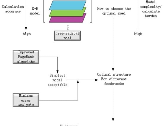
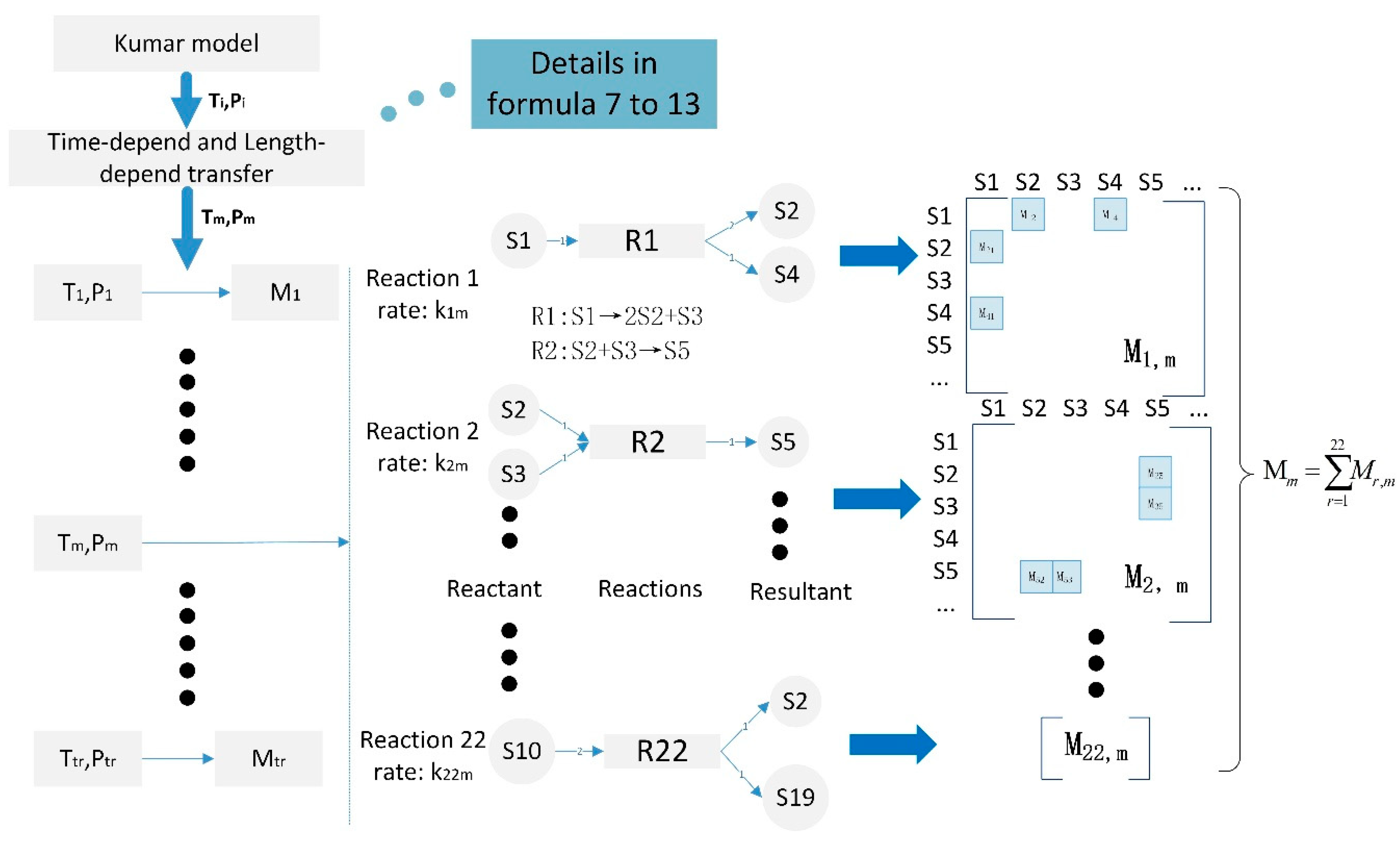
2. The Method and Basic Structural Framework of K-R Model
2.1. The Method of Enriching the Kumar Model with Free-Radical Approach
- (1).
- (2).
- The first-order reaction is convenient in optimizing the model to adapt to the change of raw material [40].
- (3).
- The approach of pyrolysis is aimed at acquiring light olefin from heavier products from the petroleum industry. For the reason that the first-order reaction is mainly linked with the heavy components reaction network, it is not necessary to be enriched.
- (1).
- Reactions of heavier reactant still have great influence on reactions among the lighter ones.
- (2).
- Double counting with the Kumar model must be avoided.
- (3).
- The reactions of reactants of the same carbon number coupled with each other greatly.
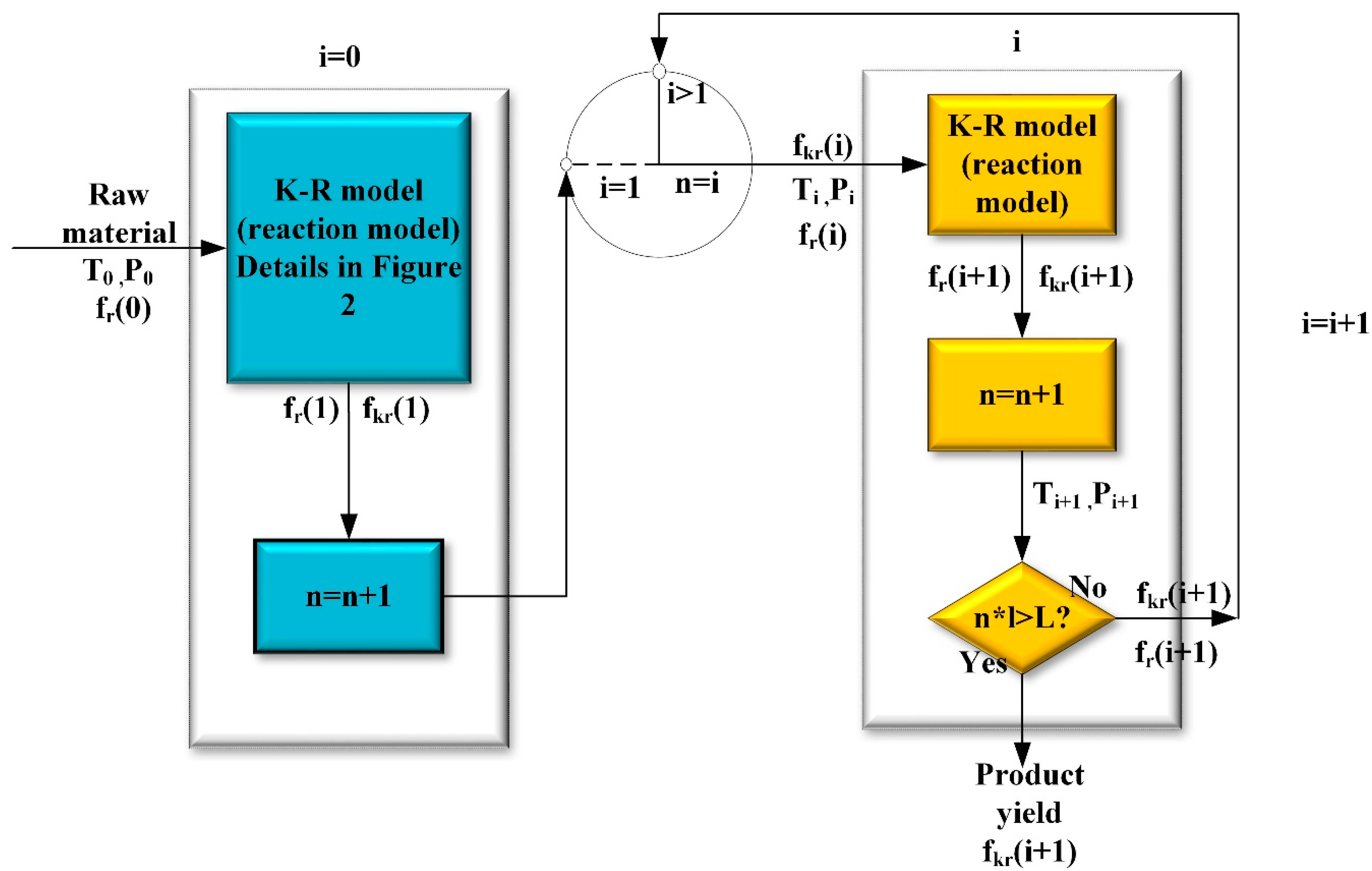
2.2. The Basic Framework of K-R Model and K-R Structure
- (1).
- The first-order reaction.
- (2).
- The modified secondary reactions
- (3).
- The supplied free-radical reaction network
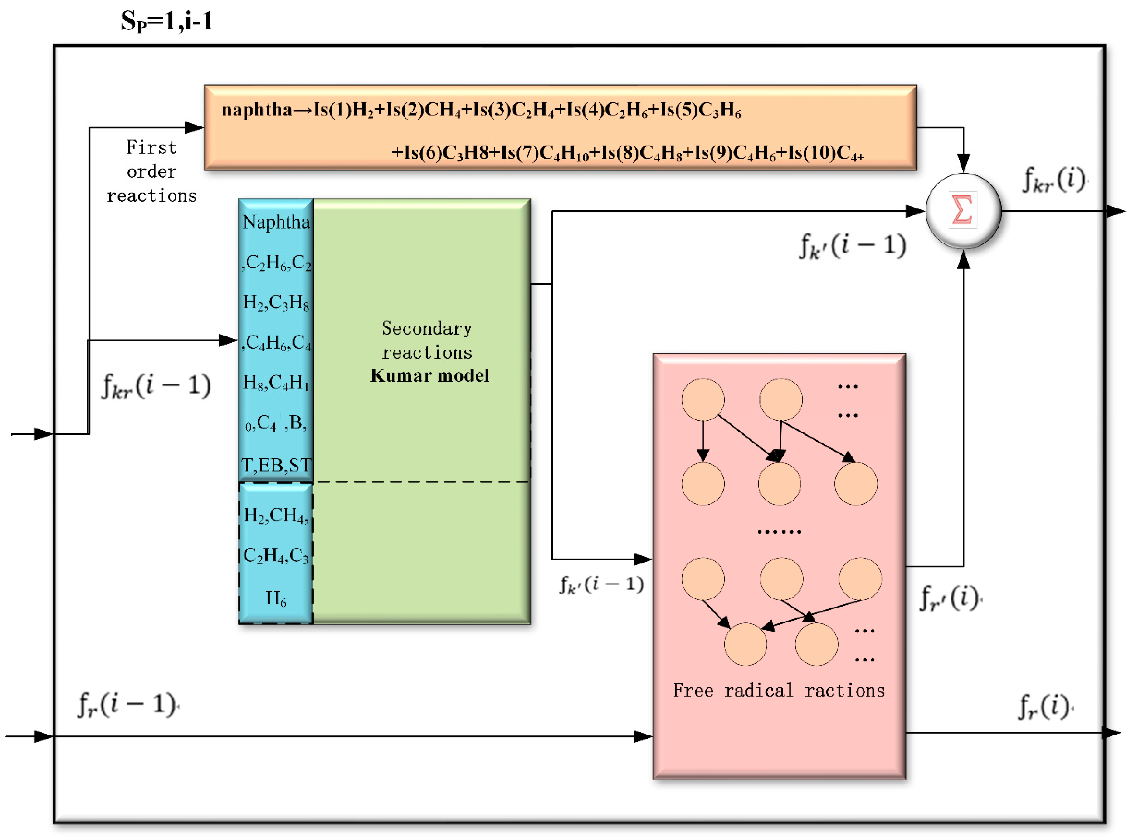
Modification of Kumar Model
- (1).
- The reactions of reactants of the same carbon number coupled with each other greatly.
- (2).
- The substances of ethylene (C2H4) and propylene (C3H6) are desired final products, which must be calculated by the free-radical approach.
- (1).
- Remove: when all the reactants belong to the scope
- (2).
- Partly Retain: Some of the reactant of the reactions belong to the scope
- (3).
- Retain: All the reactant are out of the scope
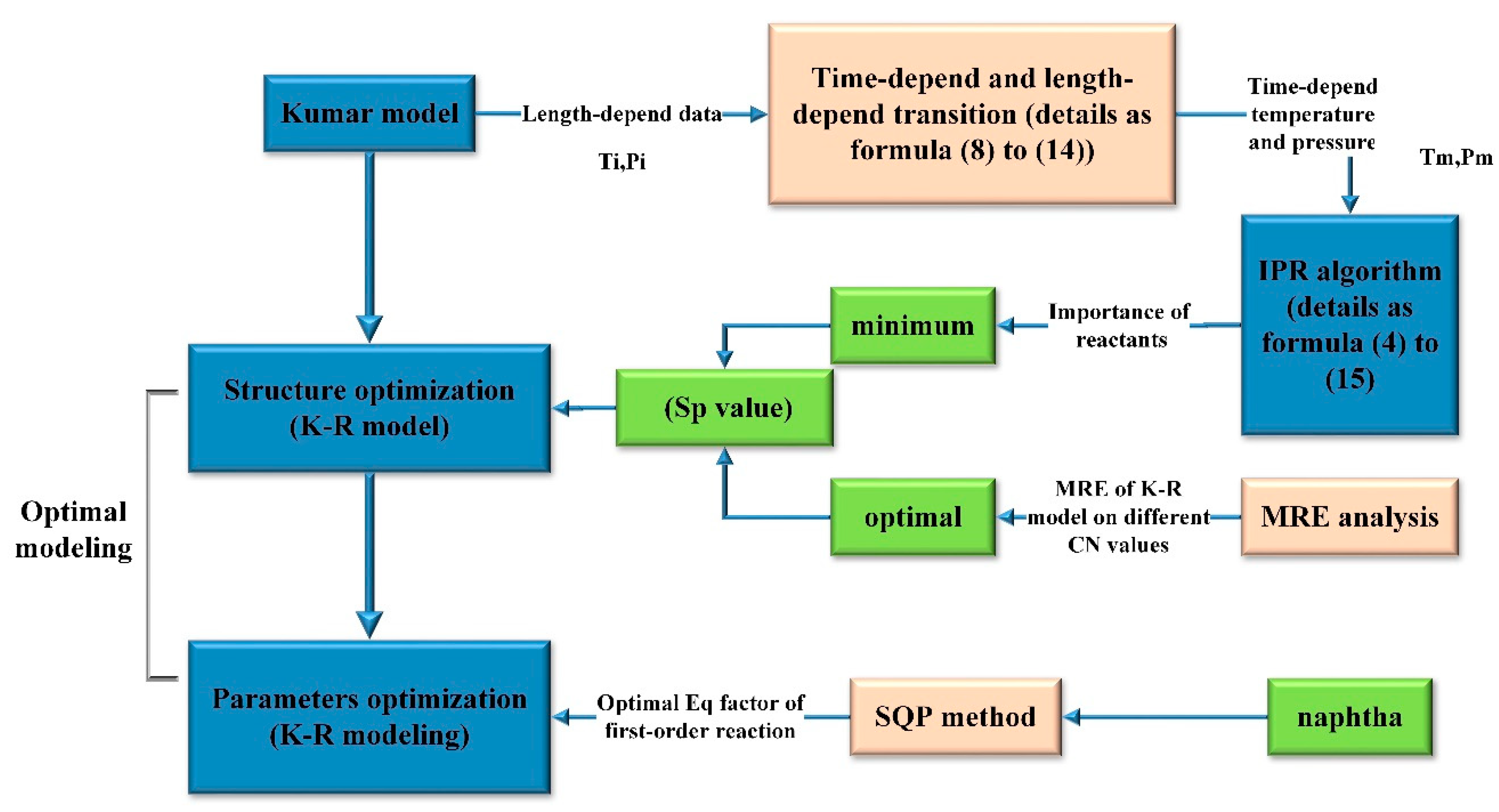
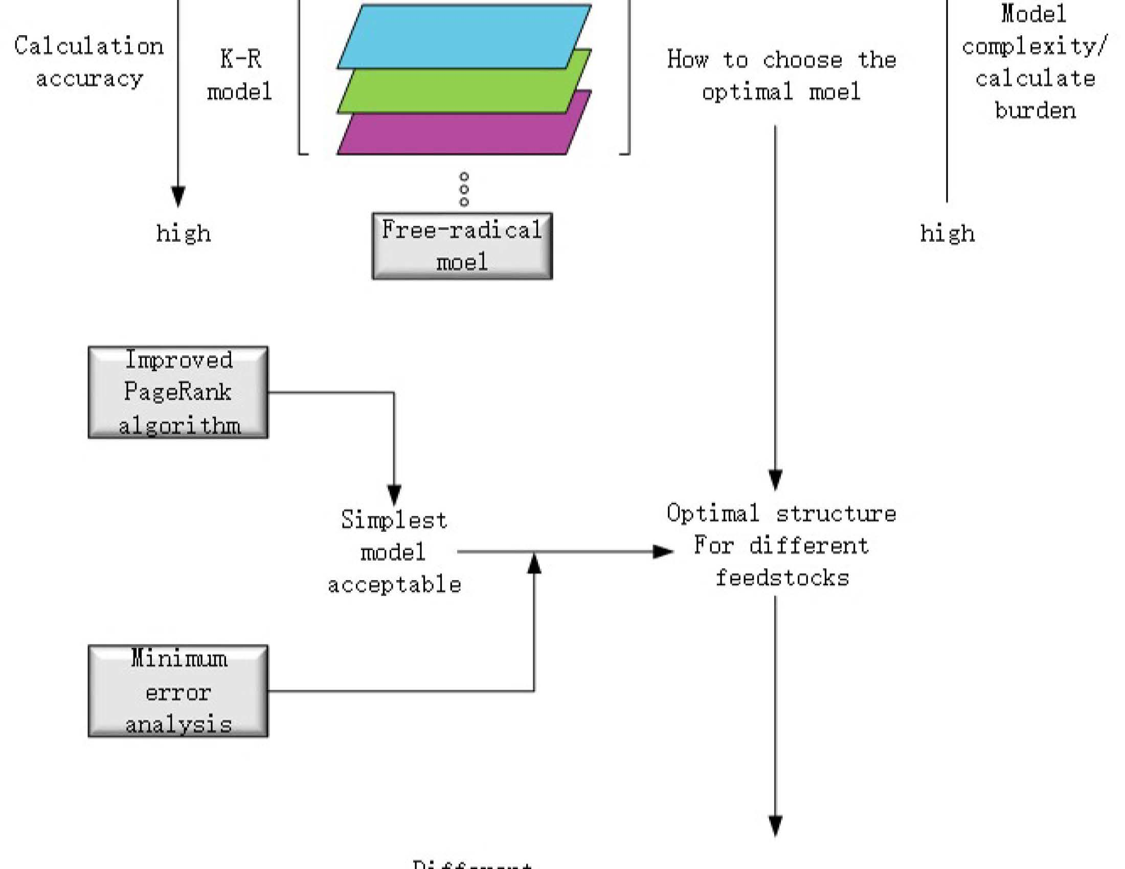
3. Optimal Modeling of K-R Model
3.1. Structure Optimization of K-R Model
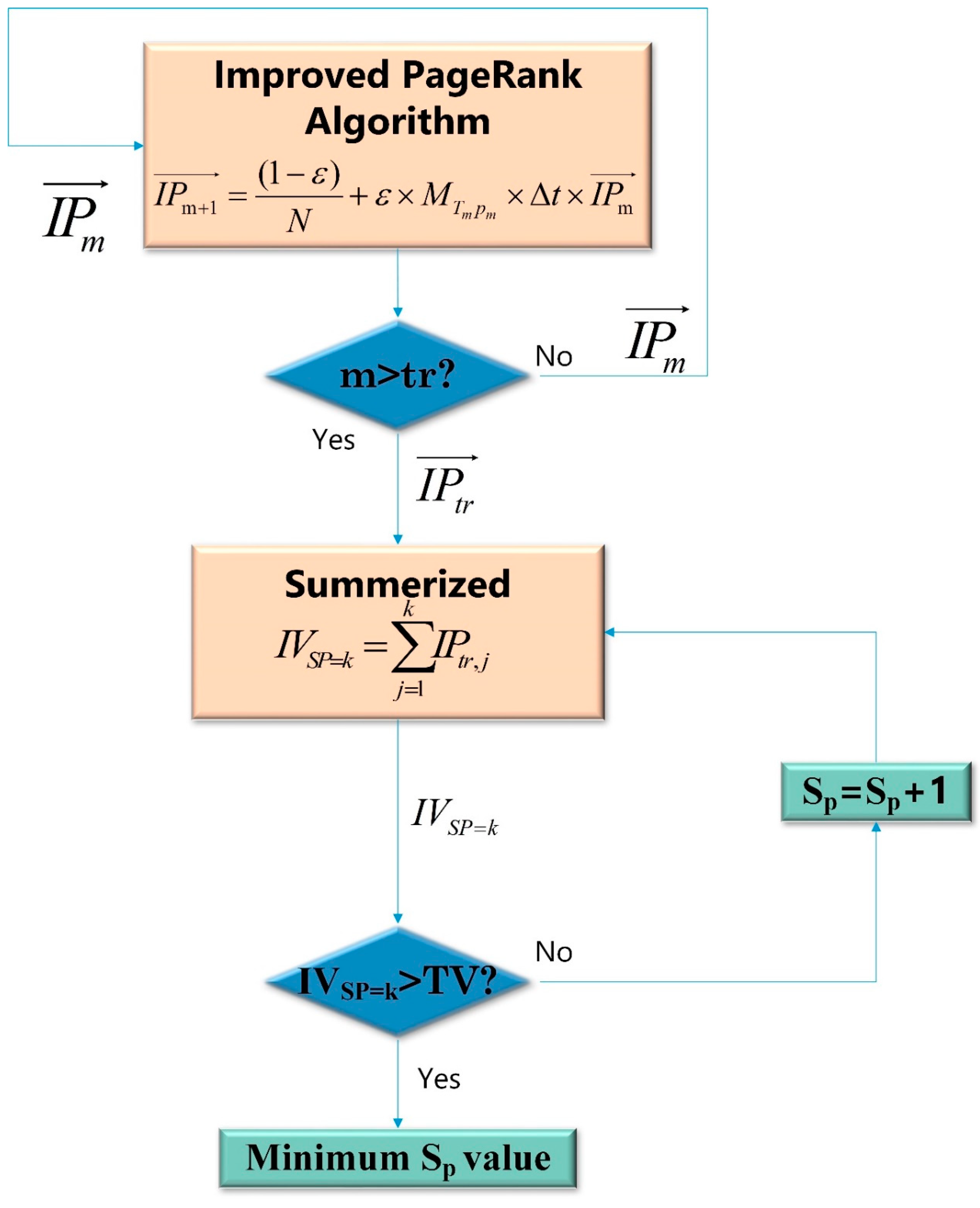
3.1.1. Minimum Scope Screened Out Via IPR Algorithm
- (1).
- The original PR algorithm keeps calculating until the values converge, which means reaction equilibration [53]. However, in a thermal cracking furnace, the reactions stop before equilibration to maximize the yield of ethylene.
- (2).
- Zhou’s PR algorithm uses the time average reaction rate to calculate the shift matrix. However, a time-dependent shift matrix may be more accurate.
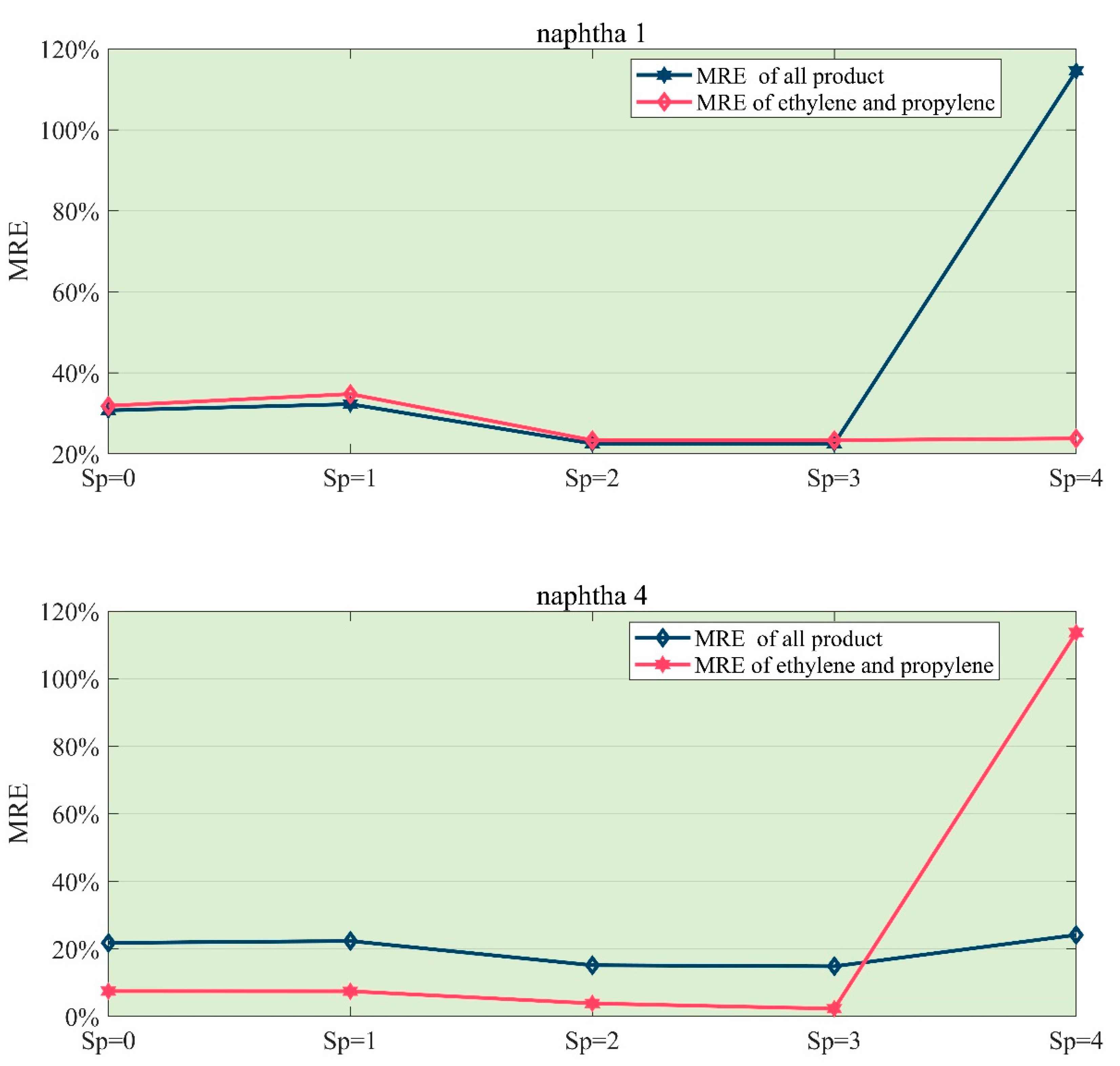
3.1.2. Optimal Scope of Enriched Reactions Based on MRE Analysis
3.2. Parameters Optimizing
4. Case Study
4.1. Case Backgrounds and Conditions
4.2. Structure Optimization of K-R Model
Screening the Minimum Sp Value of K-R Model by IPR Algorithm
4.3. Parameter Optimization on the Basis of MRE Analysis
4.4. Parameter Optimization of Value
4.5. Result Discussions
- (1).
- In the PR calculation, the parameter will influence the result. When becomes large, all important (IPj values) tend to average. When a small value is assigned to , the result will consider more about resultant. For the case study, = 0.0005 is adopted.
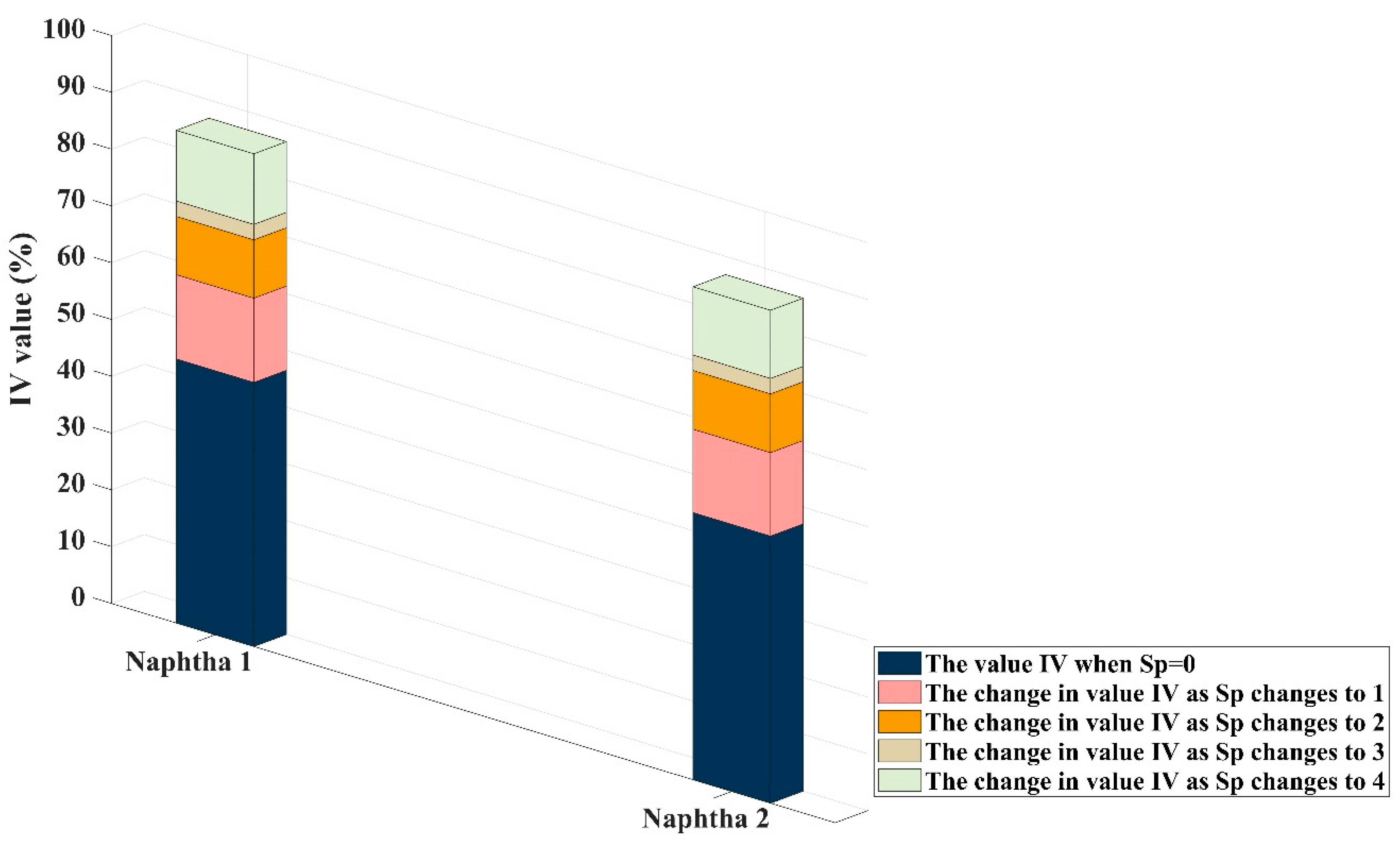
- (2).
- While performed PR calculation in conditions of different feedstock, the value of each substance may be different, but the summarized results of each Sp value are nearly the same. Results of Sp = 3 and Sp = 4 are all over 80%. This proved that the algorithm demonstrates robustness. At the same time, the difference in the calculation results between the two naphtha is mainly found in C4+, which is where Kumar’s equation ignores. The following different modeling results confirm the necessity of enhancing this part of the reaction and the correctness of the method.
- (3).
- In the simulation of naphtha, the optimal Sp value is 3. Experiments for both of the two typical feedstock indicates that if we let Sp = 4, the error of product yield will grow rapidly. The reason is that the structure of the Kumar model considers part of the reactions into the first-order reactions.
- (4).
- During the case study, we find that there are two kinds of naphtha. They performance totally different when modeling:
- (5).
- For the first kind of naphtha, like feedstocks (1), (2), and (3), both the K-R model and Kumar model can reach the accuracy of 0.06%, but the K-R model converges faster. The convergence rate of the K-R optimal modeling and Kumar optimal modeling are 35 min and 20 h respectively.
- (6).
- For the second kind of naphtha, like feedstocks (4)–(9), the Kumar model can’t get the reasonable result. Errors in ethylene (31%) and propylene (14%) are too large to accept. On the contrary, the K-R model still performs well. This difference is mainly due to the presence of isomeric reactants, and the lack of a description of such reactions is one of the weaknesses of Kumar’s model.
- (7).
- The K-R model relative errors are often very different from the Kumar relative errors (they also change from positive to negative and vice versa). This phenomenon is due to the equilibrium constraint between carbon and hydrogen.
5. Conclusions
6. Statement of Data Availability
Author Contributions
Funding
Conflicts of Interest
Nomenclature
| C4+ | Hydrocarbons containing more than four carbon atoms per molecule |
| E | The activation energy of the reaction |
| The rate constant of the reaction | |
| B | Benzene |
| T | Toluene |
| EB | Ethyl benzene |
| i-C4H8 | Isobutene |
| Structural parameters of K-R model | |
| MRE | Mean relative error |
| Mass fraction of substance | |
| Substance | |
| Reaction r | |
| The temperature at any given moment in the tube of cracking furnace | |
| The pressure at any given moment in the tube of cracking furnace | |
| The Transfer matrix for and | |
| The component of calculated by reaction r | |
| The rate of reaction r calculated by Arrhenius equation under and | |
| Reaction termination | |
| Material importance vector (iteration quantity) calculated by IPR algorithm | |
| The shift factor in IPR | |
| Number of species | |
| Iteration time per step | |
| The calculation result of material importance when | |
| TV | Threshold value |
References
- Schietekat, C.; Van Cauwenberge, D.J.; Van Geem, K.M.; Marin, G.B. Computational Fluid Dynamics-Based Design of Finned Steam Cracking Reactors. AiChE J. 2014, 60, 794–808. [Google Scholar] [CrossRef]
- Sadrameli, S.M. Thermal/catalytic cracking of liquid hydrocarbons for the production of olefins: A state-of-the-art review II: Catalytic cracking review. Fuel 2016. [Google Scholar] [CrossRef]
- Zhang, Q.; Gong, J.; Skwarczek, M.; Yue, D.; You, F. Sustainable process design and synthesis of hydrocarbon biorefinery through fast pyrolysis and hydroprocessing. AiChE J. 2014, 60, 980–994. [Google Scholar] [CrossRef]
- Chen, Z.; Xu, J.; Fan, Y.; Bao, X. Reaction mechanism and kinetic modeling of hydroisomerization and hydroaromatization of fluid catalytic cracking naphtha. Fuel Process. Technol. 2015, 130, 117–126. [Google Scholar] [CrossRef]
- Yu, K.; Wang, X.; Wang, Z. Self-adaptive multi-objective teaching-learning-based optimization and its application in ethylene cracking furnace operation optimization. Chemom. Intell. Lab. Syst. 2015, 146, 198–210. [Google Scholar] [CrossRef]
- Shirvani, S.; Ghashghaee, M. Combined effect of nanoporous diluent and steam on catalytic upgrading of fuel oil to olefins and fuels over USY catalyst. Pet. Sci. Technol. 2018, 36, 750–755. [Google Scholar] [CrossRef]
- Alvira, J.; Hita, I.; Rodríguez, E.; Arandes, J.; Castaño, P. A data-driven reaction network for the fluid catalytic cracking of waste feeds. Processes 2018, 6, 243. [Google Scholar] [CrossRef] [Green Version]
- Biswas, S.; Sharma, D.K. Studies on cracking of Jatropha oil. J. Anal. Appl. Pyrolysis 2013, 99, 122–129. [Google Scholar] [CrossRef]
- Cai, Z.; Ma, X.; Fang, S.; Yu, Z.; Lin, Y. Thermogravimetric analysis of the co-combustion of eucalyptus residues and paper mill sludge. Appl. Therm. Eng. 2016, 106, 938–943. [Google Scholar] [CrossRef]
- Shao, Y.; Guizani, C.; Grosseau, P. Thermal characterization and kinetic analysis of microfibrillated cellulose/lignosulfonate blends. J. Anal. Appl. Pyrolysis 2017, 124, 25–34. [Google Scholar] [CrossRef]
- Jeguirim, M.; Limousy, L.; Dutournie, P. Pyrolysis kinetics and physicochemical properties of agropellets produced from spent ground coffee blended with conventional biomass. Chem. Eng. Res. Des. 2014, 92, 1876–1882. [Google Scholar] [CrossRef]
- Amutio, M.; Lopez, G.; Alvarez, J. Pyrolysis kinetics of forestry residues from the Portuguese Central Inland Region. Chem. Eng. Res. Des. 2013, 91, 2682–2690. [Google Scholar] [CrossRef]
- Reyniers, P.A.; Schietekat, C.M.; Van Cauwenberge, D.J. Necessity and feasibility of 3D simulations of steam cracking reactors. Ind. Eng. Chem. Res. 2015, 54, 12270–12282. [Google Scholar] [CrossRef]
- Dente, M.; Pierucci, S.; Ranzi, E. New improvements in modeling kinetic schemes for hydrocarbons pyrolysis reactors. Chem. Eng. Sci. 1992, 47, 2629–2634. [Google Scholar] [CrossRef]
- Belohlav, Z.; Zamostny, P.; Herink, T. The kinetic model of thermal cracking for olefins production. Chem. Eng. Process. Process Intensif. 2003, 42, 461–473. [Google Scholar] [CrossRef]
- Karimi, H.; Cowperthwaite, E.V.; Olayiwola, B. Modelling of heat transfer and pyrolysis reactions in an industrial ethylene cracking furnace. Can. J. Chem. Eng. 2018, 96, 33–48. [Google Scholar] [CrossRef]
- Tangsathitkulchai, C.; Punsuwan, N.; Weerachanchai, P. Simulation of Batch Slow Pyrolysis of Biomass Materials Using the Process-Flow-Diagram COCO Simulator. Processes 2019, 7, 775. [Google Scholar] [CrossRef] [Green Version]
- Bikas, G.; Peters, N. Kinetic modelling of n-decane combustion and autoignition, Modeling combustion of n-decanem. Combust. Flame 2001, 126, 1456–1475. [Google Scholar] [CrossRef]
- Ghashghaee, M.; Ghambarian, M. Methane adsorption and hydrogen atom abstraction at diatomic radical cation metal oxo clusters: First-principles calculations. Mol. Simul. 2018, 44, 850–863. [Google Scholar] [CrossRef]
- Peng, Z.; Zhao, J.; Yin, Z. ABC-ANFIS-CTF: A Method for Diagnosis and Prediction of Coking Degree of Ethylene Cracking Furnace Tube. Processes 2019, 7, 909. [Google Scholar] [CrossRef] [Green Version]
- Geng, Z.; Cui, Y.; Xia, L. Compromising adjustment solution of primary reaction coefficients in ethylene cracking furnace modeling. Chem. Eng. Sci. 2012, 80, 16–29. [Google Scholar] [CrossRef]
- Kousha, M.; Daneshvar, E.; Dopeikar, H. Box–Behnken design optimization of Acid Black 1 dye biosorption by different brown macroalgae. Chem. Eng. J. 2012, 179, 158–168. [Google Scholar] [CrossRef]
- Szepesy, L. Feedstock characterization and prediction of product yields for industrial naphtha crackers on the basis of laboratory and bench-scale pyrolysis. J. Anal. Appl. Pyrolysis 1980, 1, 243–268. [Google Scholar] [CrossRef]
- Naik, D.V.; Singh, K.K.; Kumar, V. Catalytic cracking of glycerol to fine chemicals over equilibrium fluid catalytic cracking catalyst. Energy Procedia 2014, 54, 593–598. [Google Scholar] [CrossRef] [Green Version]
- Jin, Y.; Li, J.; Du, W. Outlet temperature correlation and prediction of transfer line exchanger in an industrial steam ethylene cracking process. Chin. J. Chem. Eng. 2013, 21, 388–394. [Google Scholar] [CrossRef]
- Keyvanloo, K.; Sedighi, M.; Towfighi, J. Genetic algorithm model development for prediction of main products in thermal cracking of naphtha: Comparison with kinetic modeling. Chem. Eng. J. 2012, 209, 255–262. [Google Scholar] [CrossRef]
- Rao, P.N.; Kunzru, D. Thermal cracking of JP-10: Kinetics and product distribution. J. Anal. Appl. Pyrolysis 2006, 76, 154–160. [Google Scholar]
- Zhang, Y.; Qian, F.; Zhang, Y. Impact of flue gas radiative properties and burner geometry in furnace simulations. AiChE J. 2015, 61, 936–954. [Google Scholar] [CrossRef]
- Rice, F.O. The Decomposition of Organic Compounds from the Standpoint of Free Radicals. Chem. Rev. 1935, 17, 53–63. [Google Scholar] [CrossRef]
- Sadrameli, S.M.; Green, A.E.S. Systematics and modeling representations of naphtha thermal cracking for olefin production. J. Anal. Appl. Pyrolysis 2005, 73, 305–313. [Google Scholar] [CrossRef]
- Zhao, Y.; Zhang, S.; Li, D. Understanding the mechanism of radical reactions in 1-hexene pyrolysis. Chem. Eng. Res. Des. 2014, 92, 453–460. [Google Scholar] [CrossRef]
- Joo, E.; Park, S.; Lee, M. Pyrolysis reaction mechanism for industrial naphtha cracking furnaces. Ind. Eng. Chem. Res. 2001, 40, 2409–2415. [Google Scholar] [CrossRef]
- Allara, D.L.; Shaw, R. A compilation of kinetic parameters for the thermal degradation of n-alkane molecules. J. Phys. Chem. Ref. Data 1980, 9, 523–560. [Google Scholar] [CrossRef] [Green Version]
- Zhao, C.; Liu, C.; Xu, Q. Cyclic scheduling for ethylene cracking furnace system with consideration of secondary ethane cracking. Ind. Eng. Chem. Res. 2010, 49, 5765–5774. [Google Scholar] [CrossRef]
- Fang, Z.; Qiu, T.; Chen, B. Analyzing and Modeling Ethylene Cracking Process with Complex Networks Approach. In Computer Aided Chemical Engineering; Elsevier: Amsterdam, The Netherlands, 2015; Volume 37, pp. 407–412. [Google Scholar]
- Pyl, S.P.; Hou, Z.; Van Geem, K.M. Modeling the composition of crude oil fractions using constrained homologous series. Ind. Eng. Chem. Res. 2011, 50, 10850–10858. [Google Scholar] [CrossRef]
- Van Damme, P.S.; Narayanan, S.; Froment, G.F. Thermal cracking of propane and propane-propylene mixtures: Pilot plant versus industrial data. AiChE J. 1975, 21, 1065–1073. [Google Scholar] [CrossRef]
- Sundaram, K.M.; Froment, G.F. A comparison of simulation models for empty tubular reactors. Chem. Eng. Sci. 1979, 34, 117–124. [Google Scholar] [CrossRef]
- Kumar, P.; Kunzru, D. Modeling of naphtha pyrolysis. Ind. Eng. Chem. Process Des. Dev. 1985, 24, 774–782. [Google Scholar] [CrossRef]
- Zhang, L.; Chen, B. Applications of Shannon’s entropy theory to naphtha pyrolysis simulation. Chem. Eng. Technol. 2012, 35, 281–286. [Google Scholar] [CrossRef]
- Yuan, B.; Li, J.; Du, W. Study on co-cracking performance of different hydrocarbon mixture in a steam pyrolysis furnace. Chin. J. Chem. Eng. 2016, 24, 1252–1262. [Google Scholar] [CrossRef]
- Chen, L.; Wang, S.; Meng, H. Synergistic effect on thermal behavior and char morphology analysis during co-pyrolysis of paulownia wood blended with different plastics waste. Appl. Therm. Eng. 2017, 111, 834–846. [Google Scholar] [CrossRef]
- Ghashghaee, M.; Shirvani, S. Two-step thermal cracking of an extra-heavy fuel oil: Experimental evaluation, characterization, and kinetics. Ind. Eng. Chem. Res. 2018, 57, 7421–7430. [Google Scholar] [CrossRef]
- Ghashghaee, M.; Shirvani, S.; Ghambarian, M. Synergistic Coconversion of Refinery Fuel Oil and Methanol over H-ZSM-5 Catalyst for Enhanced Production of Light Olefins. Energy Fuels 2019, 33, 5761–5765. [Google Scholar] [CrossRef]
- Souza, B.M.; Travalloni, L.; da Silva, M.A.P. Kinetic modeling of the thermal cracking of a Brazilian vacuum residue. Energy Fuels 2015, 29, 3024–3031. [Google Scholar] [CrossRef]
- Aridhi, S.; Lacomme, P.; Ren, L. A MapReduce-based approach for shortest path problem in large-scale networks. Eng. Appl. Artif. Intell. 2015, 41, 151–165. [Google Scholar] [CrossRef]
- Lin, Y.W.; Deng, B.C.; Wang, L.L. Fisher optimal subspace shrinkage for block variable selection with applications to NIR spectroscopic analysis. Chemom. Intell. Lab. Syst. 2016, 159, 196–204. [Google Scholar] [CrossRef]
- Ni, L.; Zhang, L.; Ni, J. Structural kinetic model of pyrolysis process of paraffins and its simulation. J. Chem. Ind. Eng. 1995, 46, 562–570. [Google Scholar]
- Simmie, J.M. Detailed chemical kinetic models for the combustion of hydrocarbon fuels. Prog. Energy Combust. Sci. 2003, 29, 599–634. [Google Scholar] [CrossRef]
- Karimzadeh, R.; Godini, H.R.; Ghashghaee, M. Flowsheeting of steam cracking furnaces. Chem. Eng. Res. Des. 2009, 87, 36–46. [Google Scholar] [CrossRef]
- Minkov, E.; Charrow, B.; Ledlie, J. Collaborative future event recommendation. In Proceedings of the 19th ACM International Conference on INFORMATION and Knowledge Management, Toronto, ON, Canada, 26–30 October 2010; pp. 819–828. [Google Scholar]
- Saha, B.; Reddy, P.K.; Ghoshal, A.K. Hybrid genetic algorithm to find the best model and the globally optimized overall kinetics parameters for thermal decomposition of plastics. Chem. Eng. J. 2008, 138, 20–29. [Google Scholar] [CrossRef]
- Acevedo, D.; Tandy, Y.; Nagy, Z.K. Multiobjective optimization of an unseeded batch cooling crystallizer for shape and size manipulation. Ind. Eng. Chem. Res. 2015, 54, 2156–2166. [Google Scholar] [CrossRef]
- Lim, W.; Lee, I.; Tak, K. Efficient configuration of a natural gas liquefaction process for energy recovery. Ind. Eng. Chem. Res. 2014, 53, 1973–1985. [Google Scholar] [CrossRef]
- Han, S.P. A successive projection method. Math. Program. 1988, 40, 1–14. [Google Scholar] [CrossRef]
- Powell, M.J.D. Algorithms for nonlinear constraints that use Lagrangian functions. Math. Program. 1978, 14, 224–248. [Google Scholar] [CrossRef]
- Zhang, L. Establishment and Application of Cracking Reaction Model. Ph.D. Dissertation, Beijing University of Chemical Technology, Beijing, China, 2012. [Google Scholar]


| No. | Reactions | E,kcal/g·mol | k0,s−1 |
|---|---|---|---|
| 1 | naphtha→0.58H2 + 0.68CH4 + 0.88C2H4 + 0.1C2H6 + 0.6C3H6 + 0.02C3H8 + 0.035C4H10 + 0.2C4H8 + 0.07C4H6 + 0.09C4+ | 52.58 | 6.565 × 10¹¹ |
| 2 | C2H6→C2H4 + H2 | 65.21 | 4.652 × 10¹³ |
| 3 | C3H6→C2H2 + CH4 | 65.33 | 7.284 × 10¹² |
| 4 | C2H2 + C2H4→C4H6 | 41.26 | 1.026 × 10¹⁵ |
| 5 | 2C2H6→C3H8 + CH4 | 65.25 | 3.75 × 10¹² |
| 6 | C2H6 + C2H6→C3H6 + CH4 | 60.43 | 7.083 × 10¹⁶ |
| 7 | C3H8→C3H6 + H2 | 51.29 | 5.888 × 10¹⁰ |
| 8 | C3H8→C2H4 + CH4 | 50.6 | 4.692 × 10¹⁰ |
| 9 | C3H8 + C2H4→C2H6 + C3H6 | 59.06 | 2.536 × 10¹⁶ |
| 10 | 2C3H6→3C2H4 | 64.17 | 7.386 × 10¹² |
| 11 | 2C3H6→0.3CnH2n-6 + 0.14C6 + + 3CH4 | 56.90 | 2.424 × 10¹¹ |
| 12 | C3H6 + C2H6→1-C4H8 + CH4 | 60.01 | 1.0 × 10¹⁷ |
| 13 | n-C4H10→C3H6 + CH4 | 59.64 | 7.0 × 10¹² |
| 14 | n-C4H10→2C2H4 + H2 | 70.68 | 7.0 × 10¹⁴ |
| 15 | n-C4H10→C2H4 + C2H6 | 61.31 | 4.099 × 10¹² |
| 16 | n-C4H10→1-C4H8 + H2 | 62.36 | 1.637 × 10¹² |
| 17 | 1-C4H8→0.41CnH2n-6 + 0.19CH6+ | 50.73 | 2.075 × 10¹¹ |
| 18 | 1-C4H8→C4H6 + H2 | 50.00 | 1.0 × 10¹⁰ |
| 19 | C2H4 + C4H6→B + 2H2 | 34.56 | 8.385 × 10¹² |
| 20 | C4H6 + C3H6→T + 2H2 | 35.64 | 9.74 × 10¹¹ |
| 21 | C4H6 + 1-C4H8→EB + 2H2 | 57.97 | 6.4 × 10¹⁷ |
| 22 | 2C4H6→ST + 2H2 | 29.76 | 1.51 × 10¹² |
| Reactions | Ea Kcal/mol | LogA s; L/mol·s | 2-C3H7 *→H * + C3H6 | 38.70 | 13.30 |
|---|---|---|---|---|---|
| C2H6→CH3 * + CH3 * | 87.5 | 16.57 | C4H7 *→H * + C4H6 | 49.30 | 14.10 |
| C3H8→CH3 * + C2H5 * | 85.0 | 16.30 | C4H7 *→C2H3 * + C2H4 | 35.15 | 11.00 |
| 2C2H4→C2H3 * + C2H5 * | 65.0 | 13.95 | 1-C4H9 *→H * + 1-C4H8 | 36.60 | 13.00 |
| C3H6→CH3 * + C2H3 * | 95.0 | 17.90 | 1-C4H9 *→C2H5 * + C2H4 | 28.00 | 12.20 |
| 2C3H6→C3H5 * + 1-C3H7 * | 51.0 | 11.54 | 2-C4H9 *→CH3 * + C3H6 | 31.90 | 13.40 |
| H * + C2H6→H2 + C2H5 * | 9.70 | 11.08 | 2-C4H9 *→H * + 1-C4H8 | 39.80 | 13.30 |
| H * + C3H8→H2 + 1-C3H7 * | 9.70 | 11.00 | 2-C4H9 *→H * + 2-C4H8 | 37.90 | 12.70 |
| H * + C3H8→H2 + 2-C3H7 * | 8.30 | 10.95 | C5H9 *→CH3 * + C4H6 | 38.00 | 12.90 |
| H * + C2H4→H2 + C2H3 * | 4.00 | 8.50 | C5H9 *→C2H3 * + C3H6 | 34.00 | 13.20 |
| H * + C3H6→H2 + C3H5 * | 4.50 | 8.50 | C5H9 *→C3H5 * + C2H4 | 34.00 | 13.20 |
| CH3 * + C2H6→CH4 + C2H5 * | 15.25 | 10.20 | 1-C5H11 *→C2H4 + 1-C3H7 * | 32.70 | 13.70 |
| CH3 * + C3H8→CH4 + 1-C3H7 * | 12.70 | 10.10 | 2-C5H11 *→C2H5 * + C3H6 | 29.10 | 12.70 |
| CH3 * + C3H8→CH4 + 2-C3H7 * | 10.80 | 10.10 | H * + CH3 *→CH4 | 0 | 9.86 |
| CH3 * + C2H4→CH4 + C2H3 * | 13.00 | 8.60 | H * + C2H3 *→C2H4 | 0 | 10.00 |
| CH3 * + C3H6→CH4 + C3H5 * | 4.50 | 7.30 | H * + C3H5 *→C3H6 | 0 | 10.30 |
| C2H5 * + C3H8→C2H6 + 1-C3H7 * | 12.60 | 8.70 | H * + C2H5 *→C2H6 | 0 | 10.50 |
| C2H5 * + C3H8→C2H6 + 2-C3H7 * | 10.40 | 8.70 | H * + 1-C3H7 *→C3H8 | 0 | 10.00 |
| C2H5 * + C2H4→C3H6 + CH3 * | 19.00 | 9.15 | H * + 2-C3H7 *→C3H8 | 0 | 10.00 |
| C2H5 * + C3H6→C2H6 + C3H5 * | 9.20 | 8.65 | H * + 1-C4H9 *→n-C4H10 | 0 | 10.00 |
| C2H5 * + C3H8→C2H4 + C3H5 * | 14.50 | 10.20 | H * + 2-C4H9 *→n-C4H10 | 0 | 10.00 |
| C3H5 * + C3H8→C3H6 + 1-C3H7 * | 18.80 | 9.00 | H * + C4H7 *→1-C4H8 | 0 | 10.30 |
| C3H5 * + C3H8→C3H6 + 1-C3H7 * | 16.20 | 8.90 | H* + C5H9 *→C5H10 | 0 | 10.34 |
| H * + C2H4→C2H5 * | 1.30 | 10.65 | CH3 * + CH3 *→C2H6 | 0 | 10.00 |
| H * + C3H6→1-C3H7 * | 2.90 | 10.00 | CH3 * + C2H5 *→C3H8 | 0 | 10.00 |
| H * + C3H6→2-C3H7 * | 1.50 | 10.00 | CH3 * + 1-C3H7 *→n-C4H10 | 0 | 9.51 |
| H * + C2H2→C2H3 * | 1.30 | 10.60 | CH3 * + 2-C3H7 *→n-C4H10 | 0 | 9.51 |
| H * + C3H4→C3H5 * | 1.50 | 10.00 | CH3 * + 1-C4H9 *→C5H12 | 0 | 10.11 |
| H * + C4H6→C4H7 * | 1.30 | 10.60 | CH3 * + C2H3 *→C3H6 | 0 | 10.86 |
| CH3 * + C2H4→1-C3H7 * | 7.80 | 8.60 | CH3 * + C3H5 *→1-C4H8 | 0 | 11.00 |
| CH3 * + C3H6→2-C4H9 * | 7.40 | 8.51 | CH3 * + C4H7 *→C5H10 | 0 | 9.51 |
| CH3 * + C4H6→C5H9 * | 4.10 | 7.90 | C2H5 * + C2H5 *→n-C4H10 | 0 | 8.60 |
| C2H5 * + C2H4→1-C4H9 * | 7.60 | 7.80 | C2H5 * + 1-C3H7 *→n-C5H12 | 0 | 8.90 |
| C2H5 * + C3H6→2-C5H11 * | 7.50 | 7.50 | C2H5 * + C2H3 *→1-C4H8 | 0 | 9.00 |
| 1-C3H7 * + C2H4→1-C5H11 * | 7.40 | 7.80 | C2H5 * + C3H5 *→C5H10 | 0 | 9.51 |
| C2H3 * + C2H4→C4H7 * | 7.65 | 7.65 | C2H5 * + C2H3 *→C4H6 | 0 | 8.00 |
| C2H3 * + C3H6→C5H9 * | 8.00 | 7.00 | C2H5 * + C2H5 *→C2H6 + C2H4 | 0 | 7.70 |
| C3H5 * + C2H4→C5H9 * | 8.00 | 7.00 | C2H5 * + C3H5 *→C2H6 + C3H4 | 0 | 8.60 |
| C2H3 *→H * + C2H2 | 31.50 | 9.30 | C2H5 * + C3H5 *→C2H4 + C3H6 | 0 | 8.60 |
| C2H5 *→H * + C2H4 | 40.90 | 13.90 | C2H5 * + C4H7 *→C2H6 + C4H6 | 0 | 9.11 |
| C3H5 *→H * + C3H4 | 48.00 | 12.84 | C2H5 * + C4H7 *→C2H4 + 1-C4H8 | 0 | 8.51 |
| C3H5 *→CH3 * + C2H2 | 36.00 | 10.48 | C3H5 * + C4H7 *→C3H6 + C4H6 | 0 | 10.00 |
| 1-C3H7 *→H * + C3H6 | 38.40 | 13.30 | C3H5 * + C4H7 *→C3H4 + 1-C4H8 | 0 | 9.00 |
| 1-C3H7 *→CH3 * + C2H4 | 34.00 | 13.70 | C4H7 * + C4H7 *→C4H6 + 1-C4H8 | 0 | 9.51 |
| Rank of Species (j) | Substance | 5 | C2H6 | 10 | C4H6 | 15 | n-C4H10 |
|---|---|---|---|---|---|---|---|
| 1 | Naphtha | 6 | C3H6 | 11 | C4+ | 16 | B |
| 2 | H2 | 7 | C3H8 | 12 | C2H2 | 17 | T |
| 3 | CH4 | 8 | C4H10 | 13 | CnH2n-6 | 18 | EB |
| 4 | C2H4 | 9 | C4H8 | 14 | i-C4H8 | 19 | ST |
| Sp Value | 1 | 2 | 3 | 4 | |
|---|---|---|---|---|---|
| Content been calculated by- | Residual Kumar model | Naphtha, C2H6, C2H2, C3H8, C4H6, C4H8, C4H10, C4+, B, T, EB, ST | Naphtha, C3H8, C4H6, C4H8, C4H10, C4+, B, T, EB, ST | Naphtha, C4H6, C4H8, C4H10, C4+, B, T, EB, ST | Naphtha, C4+, B, T, EB, ST |
| Free-radical approach | H2, CH4, C2H4, C3H6 | H2, CH4, C2H4, C3H6, C2H6, C2H2 | H2, CH4, C2H4, C3H6, C2H6, C2H2, C3H8 | H2, CH4, C2H4, C3H6, C2H6, C2H2, C3H8, C4H6, C4H8, C4H10 | |
| Structure Parameter | Value | Operational Conditions | Value |
|---|---|---|---|
| Furnace tube group | 6 | Feedstock flow (kg/h) | 890.625 |
| Tube pass | 2 | Steam/Hydrocarbon ratio | 0.60 |
| Arrangement | 16/8 | Coil inlet temperature (K) | 875 |
| Inner diameter (m) | 0.051/0.073 | Coil outlet temperature (K) | 1122 |
| Outer diameter (m) | 0.063/0.086 | Coil outlet pressure (kPa) | 178 |
| Length (m) | 13.681/14.921 | ||
| Tube pitch (m) | 0.112/0.154 |
| Naphtha | 1 | 2 | 3 | 4 | 5 | 6 | 7 | 8 | 9 |
|---|---|---|---|---|---|---|---|---|---|
| Density (20 °C, g/cm3) | 0.6927 | 0.7255 | 0.7488 | 0.7022 | 0.7103 | 0.7389 | 0.7093 | 0.7375 | 0.6894 |
| ASTM, °C (10%) | 54.5 | 86.9 | 85.2 | 60 | 64 | 77 | 69 | 85.2 | 36.2 |
| ASTM, °C (30%) | 73 | 105.4 | 114.8 | 75 | 81 | 106 | 88 | 105 | 46.9 |
| ASTM, °C (50%) | 90 | 121.3 | 131.8 | 88.5 | 98 | 135 | 103 | 120.3 | 65 |
| ASTM, °C (70%) | 107 | 137.3 | 147.5 | 103 | 117 | 163 | 119 | 136.2 | 104.7 |
| ASTM, °C (90%) | 127 | 156.5 | 162.4 | 124 | 143 | 190 | 149 | 156.1 | 137.6 |
| P/N/A | 0.7223/0.2234/0.0529 | 0.663/0.2605/0.0762 | 0.4631/0.4856/0.0483 | 0.7069/0.2248/0.0566 | 0.6669/0.2605/0.068 | 0.6898/0.1916/0.116 | 0.6409/0.3172/0.0419 | 0.5609/0.3493/0.0893 | 0.7379/0.1742/0.0864 |
| Substance | IPj Value (%) | C4+ | 5.330676 |
|---|---|---|---|
| H2 | 9.397315 | C2H2 | 2.540632 |
| CH4 | 14.82913 | CnH2n-6 | 3.362184 |
| C2H4 | 19.02015 | I-C4H8 | 5.990581 |
| C2H6 | 4.373818 | N-C4H10 | 2.613754 |
| C3H6 | 8.31053 | B | 2.877133 |
| C3H8 | 2.715596 | T | 2.550521 |
| C4H10 | 2.634325 | EB | 2.583697 |
| C4H8 | 3.786447 | ST | 2.587514 |
| C4H6 | 4.49599 |
| Substance | IPj Value (%) | C4+ | 4.86766 |
|---|---|---|---|
| H2 | 9.056091 | C2H2 | 2.530207 |
| CH4 | 14.6854 | CnH2n-6 | 3.339963 |
| C2H4 | 19.70367 | I-C4H8 | 5.933869 |
| C2H6 | 4.47801 | N-C4H10 | 2.598407 |
| C3H6 | 8.586633 | B | 2.887175 |
| C3H8 | 2.719097 | T | 2.54081 |
| C4H10 | 2.617593 | EB | 2.573647 |
| C4H8 | 3.757652 | ST | 2.579013 |
| C4H6 | 4.545106 |
| Substance | Target Yields (wt %) | Kumar Yields (wt %) | Relative Errors 1 (%) | K-R Model Yields (wt %) | Relative Errors 2 (%) |
|---|---|---|---|---|---|
| H2 | 1.09 | 1.2776 | 17.211 | 0.8733 | −19.880733 |
| CH4 | 16.85 | 12.86 | −23.6795 | 13.0195 | −22.7329 |
| C2H4 | 28.83 | 27.386 | −5.00867 | 28.5798 | −0.86785 |
| C2H6 | 2.86 | 2.006 | −29.8601 | 3.56 | 24.4755 |
| C3H6 | 13 | 17.163 | 32.02307 | 15.7391 | 21.07 |
| C4H8 | 3.43 | 3.4139 | −0.4694 | 3.55 | 3.49854 |
| C4H6 | 4.64 | 3.3741 | −27.2823 | 3.72 | −19.8276 |
| MRE (%) | 22.49 | 18.36 |
| Substance | Target Yields (wt %) | Kumar Yields (wt %) | Relative Errors 1 (%) | K-R Model Yields (wt %) | Relative Errors 2 (%) |
|---|---|---|---|---|---|
| H2 | 1.06 | 1.2567 | 18.5566 | 0.8532 | −19.5094 |
| CH4 | 16.57 | 12.656 | −23.621 | 12.8766 | −22.2897 |
| C2H4 | 30.22 | 26.952 | −10.814 | 30.0053 | −0.71046 |
| C2H6 | 3.08 | 1.9732 | −35.9351 | 3.7749 | 22.56169 |
| C3H6 | 13.61 | 16.877 | 24.00441 | 16.6434 | 22.28802 |
| C4H8 | 3.48 | 3.3509 | −3.70977 | 3.5067 | 0.767241 |
| C4H6 | 4.76 | 3.3244 | −30.1597 | 3.6635 | −23.0357 |
| MRE (%) | 23.33 | 18.57 |
| Substance | Target Yields (wt %) | Kumar Yields (wt %) | Relative Errors 1 (%) | Optimized K-R Model Yields (wt %) | Relative Errors 2 (%) |
|---|---|---|---|---|---|
| H2 | 1.09 | 1.091 | 0.091743 | 1.0903 | 0.027523 |
| CH4 | 16.85 | 16.854 | 0.023739 | 16.8625 | 0.074184 |
| C2H4 | 28.83 | 28.837 | 0.024280 | 28.8375 | 0.026015 |
| C2H6 | 2.86 | 2.8602 | 0.006993 | 2.861 | 0.034965 |
| C3H6 | 13 | 13.002 | 0.015385 | 13.0024 | 0.018462 |
| C4H8 | 3.43 | 3.4285 | −0.043732 | 3.4321 | 0.061224 |
| C4H6 | 4.64 | 4.6399 | −0.002155 | 4.6385 | −0.03233 |
| MRE (%) | 0.04 | 0.04 |
| Substance | Target Yields (wt %) | Kumar Yields (wt %) | Relative Errors 1 (%) | Optimized K-R Model Yields (wt %) | Relative Errors 2 (%) |
|---|---|---|---|---|---|
| H2 | 1.06 | 1.2567 | 0.996241 | 1.0595 | −0.04717 |
| CH4 | 16.57 | 12.656 | 16.93835 | 16.5834 | 0.080869 |
| C2H4 | 30.22 | 26.952 | 30.97339 | 30.2132 | −0.0225 |
| C2H6 | 3.08 | 1.9732 | 3.267048 | 3.0814 | 0.045455 |
| C3H6 | 13.61 | 16.877 | 14.40224 | 13.6173 | 0.053637 |
| C4H8 | 3.48 | 3.3509 | 3.782969 | 3.4765 | −0.10057 |
| C4H6 | 4.76 | 3.3244 | 5.025989 | 4.7621 | 0.044118 |
| MRE (%) | 5.67 | 0.061 |
| Naphtha (1) | Is Value | Naphtha (4) | Is Value |
|---|---|---|---|
| 1. H2 | 0.4682 | 1. H2 | 0.4469 |
| 2. CH4 | 0.9799 | 2. CH4 | 0.9883 |
| 3. C2H4 | 0.9783 | 3. C2H4 | 1.0333 |
| 4. C2H6 | 0.1450 | 4. C2H6 | 0.1571 |
| 5. C3H6 | 0.4602 | 5. C3H6 | 0.4926 |
| 6. C3H8 | 0.0089 | 6. C3H8 | 0.0098 |
| 7. C4H10 | 0.0144 | 7. C4H10 | 0.0137 |
| 8. C4H8 | 0.1998 | 8. C4H8 | 0.2008 |
| 9. C4H6 | 0.1072 | 9. C4H6 | 0.1123 |
| 10. C4+ | 0.1932 | 10. C4+ | 0.1605 |
© 2020 by the authors. Licensee MDPI, Basel, Switzerland. This article is an open access article distributed under the terms and conditions of the Creative Commons Attribution (CC BY) license (http://creativecommons.org/licenses/by/4.0/).
Share and Cite
Mu, P.; Gu, X. Thermal Cracking Furnace Optimal Modeling Based on Enriched Kumar Model by Free-Radical Reactions. Processes 2020, 8, 91. https://doi.org/10.3390/pr8010091
Mu P, Gu X. Thermal Cracking Furnace Optimal Modeling Based on Enriched Kumar Model by Free-Radical Reactions. Processes. 2020; 8(1):91. https://doi.org/10.3390/pr8010091
Chicago/Turabian StyleMu, Peng, and Xiangbai Gu. 2020. "Thermal Cracking Furnace Optimal Modeling Based on Enriched Kumar Model by Free-Radical Reactions" Processes 8, no. 1: 91. https://doi.org/10.3390/pr8010091
APA StyleMu, P., & Gu, X. (2020). Thermal Cracking Furnace Optimal Modeling Based on Enriched Kumar Model by Free-Radical Reactions. Processes, 8(1), 91. https://doi.org/10.3390/pr8010091