Estimation of Actuator and System Faults Via an Unknown Input Interval Observer for Takagi–Sugeno Systems

Abstract

This paper presents a simultaneous state variables and system and actuator fault estimation, based on an unknown input interval observer design for a discrete-time parametric uncertain Takagi–Sugeno system under actuator fault, with disturbances in the process and measurement noise. The observer design is synthesized by considering unknown but bounded process disturbances, output noise, as well as bounded parametric uncertainties. By taking into account these considerations, the upper and lower bounds of the considered faults are estimated. The gain of the unknown input interval observer is computed through a linear matrix inequalities (LMIs) approach using the robust $H_{\infty }$ criteria in order to ensure attenuation of process disturbances and output noise. The interval observer scheme is experimentally evaluated by estimating the upper and lower bounds of a torque load perturbation, a friction parameter and a fault in the input voltage of a permanent magnet DC motor.

1. Introduction

Typically, an observer is an scheme for state estimation through the system input and output measurements. For instance, in [1] a nonlinear observer is applied to estimate the degree of polymerization in a series of polycondensation reactors. However, an observer can be designed for parameter estimation [2], unknown input estimation [3,4] or fault estimation [5,6] among other important applications where it is important to precisely know the actual value of the states, signals or parameters for multiple purposes.

Sometimes there are many technical difficulties in performing an exact estimation of the state, signals or parameters to be estimated. For instance: (i) Model uncertainties, (ii) simplifying assumptions of physical phenomena for modeling, and (iii) complexity reduction of models or the unmeasured disturbances, represent an important source of mismatch between a real process and a mathematical model. In these cases, an approximation of the estimated values can be performed. These approximations can be very useful in many applications where there is not necessary to know the exact value of a variable.

An alternative to estimate unknown variables in processes with uncertain models, interval observers can be used. These observers provide an interval estimation providing a lower and upper bound of the unknown estimated variables. The actual value of the corresponding unmeasured variable located inside the interval defined by these bounds assuming that the uncertainty bounds are known.

Although it is not possible to estimate the exact value of a variable, the information provided by an interval observer can be very useful for several applications. For instance, the authors in [7] propose an interval observer to estimate the lower and upper bounds of vehicle dynamics regardless of the presence of unknown inputs whose bounded interval is also estimated. The authors in [8] design an interval sliding mode observer for sensor fault detection and applied it to an electrical traction device. Another interesting application of interval observers is given in [9], where a trajectory control based on an interval observer is designed for a quadrotor. The interval observer is synthesized by using an uncertain model where all the uncertainties (parameters, disturbance, noise) are unknown but bounded with known bounds.

The main limitation of recent works regarding interval observers is that in most cases, the interval observer design considers linear systems, or a very particular structure of nonlinear systems which sometimes are transformed into linear ones. For instance, the observer in [7] has been designed for switched systems; therefore, its use is limited. In other cases of interval observer designs such as [9], no faults are considered to be estimated or there is a lack of procedure to detect actuator faults [8].

The objective of this paper is to design an interval observer for a wider variety of nonlinear processes by using the Takagi–Sugeno (T–S) approach. Most of the nonlinear models can be adequately transformed into a T–S model (e.g., [10,11]) by using two different methods [12]:

• The nonlinear sector method, in this case the nonlinear model and its equivalent T–S model have exactly the same behavior. For this reason, this is the method used in this work.
• The linearization method, in which the equivalent T–S model can be dynamically approximated to the original nonlinear model with a certain accuracy, depending on the design requirements.

Besides, many advantageous opportunities arise when interval observers are designed for processes modeled in T–S form: (i) Pole placement via linear matrix inequalities (LMI) regions is considered to compute the observer gains, in contrast with many nonlinear approaches where the observer gains are heuristically tuned; (ii) a standard methodological procedure can be used to compute the observer gains; (iii) many approaches originally conceived for linear systems can be easily extended to T–S systems. For these reasons, the design of interval observers for T–S systems is a recent and interesting research topic. For example in [13], the authors propose an interval observer for the state estimation of systems modeled in T–S form with parametric uncertainty, disturbances, and measurement noise. However, the work is limited to estimate the unmeasured states. The authors in [14] treat the problem of fault diagnosis of proton exchange membrane (PEM) fuel cells. However, this paper deals with only the case of sensor faults by means of a bank of observers. In [15] a robust fault detection procedure for vehicle lateral dynamics using a switched T–S interval observer is presented. The proposed method is conceived to detect but not to estimate faults.

The main contribution of this paper consists in the design of an interval observer that performs a simultaneous estimation of unmeasured states, actuator and system faults for processes modeled in T–S form with uncertainties. The conditions for the existence of such observers are given. Such conditions guarantee the observer stability and they are proved through a Lyapunov analysis combined with a LMI formulation. The interval observer scheme is experimentally evaluated by estimating the upper and lower bounds of a torque load perturbation, a friction parameter and a fault in the input voltage of a permanent magnet direct-current (DC) motor. These cases are typical faults that, if not detected in time, can become catastrophic failures such as short-circuits or machinery damages due to damaged bearings.

2. Problem Formulation and Preliminaries

Consider the following discrete-time T–S system:

$$\begin{array}{cc}\hfill x(k+1)& {\displaystyle =\sum _{i=1}^m{\xi }_i\left(\rho \left(k\right)\right)[(A_i+\Delta A_i)x\left(k\right)+B_{i}u\left(k\right)]+E_{f}f\left(k\right)+G\theta \left(k\right)+E_{w}w\left(k\right),}\hfill \\ \hfill y\left(k\right)& =Cx\left(k\right)+E_{v}v\left(k\right),\hfill \end{array}$$

(1)

where $x\left(k\right)\in {\mathbb{R}}^{n_x}$, $u\left(k\right)\in {\mathbb{R}}^{n_u}$, $f\left(k\right)\in {\mathbb{R}}^{n_f}$, $\theta \left(k\right)\in {\mathbb{R}}^{n_{\theta }}$, $w\left(k\right)\in {\mathbb{R}}^{n_w}$ and $v\left(k\right)\in {\mathbb{R}}^{n_v}$ represent the state variable, the input, the actuators fault vector, the unknown parameter, the disturbance and the output noise vector. $A_i,\Delta A_i,B_i,G$ and C are matrices of appropriate dimensions. $E_f,E_w$ and $E_v$ are matrices of the coupling distribution. k denotes the $k-$th discrete time instant.

The term ${\displaystyle {\xi }_i\left(\rho \left(k\right)\right)}$ represents the i-th membership function, which is a weighting of the rule i, where $i=1,2,\cdots ,m$. The membership functions are normalized, i.e., they satisfy the following conditions [12,16]:

$$\left\{\begin{array}{c}{\displaystyle \sum _{i=1}^m{\xi }_i\left(\rho \left(k\right)\right)=1}\hfill \\ 0\le {\xi }_i\left(\rho \left(k\right)\right)\le 1,i=1,2,\cdots ,m.\hfill \end{array}\right.$$

(2)

To obtained a simultaneous estimation of parameters and faults, the system (1) is rewritten as follows

$$\begin{array}{cc}\hfill x(k+1)& =\sum _{i=1}^m{\xi }_i\left(\rho \left(k\right)\right)(A_i+\Delta A_i)x\left(k\right)+B_{i}u\left(k\right)+\overline{E}{f}_{\overline{E}}\left(k\right)+E_{w}w\left(k\right)\hfill \\ \hfill y\left(k\right)& =Cx\left(k\right)+E_{v}v\left(k\right),\hfill \end{array}$$

(3)

where the vector $f_{\overline{E}}\left(k\right)$ is an augmented one, which is defined by the actuator fault vector $f\left(k\right)$ and the unknown parameter vector $\theta \left(k\right)$; and consequently, the matrix $\overline{E}$ contains the fault coupling distribution matrix $E_f$ and the parameter matrix G, i.e.,:

$$\overline{E}=\left[\begin{array}{cc}{E}_f& G\end{array}\right],f_{\overline{E}}\left(k\right)=\left[\begin{array}{c}f\left(k\right)\\ \theta \left(k\right)\end{array}\right].$$

The following considerations are taken into account for the T–S system of the Equation (3):

• The augmented fault vector $f_{\overline{E}}\left(k\right)$ is defined as:

  $$f_{\overline{E}}(k+1)=f_{\overline{E}}\left(k\right)+w_{f_{\overline{E}}}\left(k\right),$$

  (4)

  where $w_{f_{\overline{E}}}\left(k\right)$ is considered as a variation of the actuator fault. Therefore, the estimation of $f_{\overline{E}}\left(k\right)$ is equivalent to the estimation of $\widehat{f}\left(k\right)$ and $\widehat{\theta }\left(k\right)$.
• The perturbation vector $w\left(k\right)$ is considered unknown but bounded as follows:

  $$\overline{w}\left(k\right)\le w\left(k\right)\le \underline{w}\left(k\right).$$

  (5)
• The noise vector $v\left(k\right)$ is also considered as an unknown but bounded signal, i.e.,:

  $$|v(k)|\le V\left(k\right).$$

  (6)
• The uncertain matrix $\Delta A_i$ is considered bounded as follows,

  $$\overline{\Delta A_i}\le \Delta A_i\le \underline{\Delta A_i}.$$

  (7)
• Based on previous assumptions, the estimates to be obtained will be as follows

  $$\overline{\widehat{x}}\left(k\right)\le x\left(k\right)\le \underline{\widehat{x}}\left(k\right),$$

  (8)

  $${\overline{\widehat{f}}}_{\overline{E}}\left(k\right)\le f_{\overline{E}}\left(k\right)\le {\widehat{\underline{f}}}_{\overline{E}}\left(k\right).$$

  (9)

This means that we would get two estimates, i.e., the upper and lower limit of each variable. For that, we consider the following design based on a T–S interval observer.

3. Observer Design

In this section a similar procedure as that in [17] (where no parametric uncertainties nor noise nor disturbances were considered) is presented for the observer design. For this design, first it is considered the output vector at time instant $(k+1)$, i.e.,

$$y(k+1)=Cx(k+1)+E_{v}v(k+1).$$

(10)

Substituting the state equation from system (3), it yields to:

$$\begin{array}{cc}\hfill y(k+1)& =C\left(\sum _{i=1}^m{\xi }_i\left(\rho \left(k\right)\right)[(A_i+\Delta A_i)x\left(k\right)+B_{i}u\left(k\right)]+{\overline{E}}_{f\overline{E}}\left(k\right)+E_{w}w\left(k\right)\right)+E_{v}v(k+1).\hfill \end{array}$$

(11)

Next, the following equation can be derived after the pertinent operations

$$\begin{array}{cc}\hfill C{\overline{E}}_{f\overline{E}}\left(k\right)=& y(k+1)-C\sum _{i=1}^m{\xi }_i\left(\rho \left(k\right)\right)(A_i+\Delta A_i)x\left(k\right)-C\sum _{i=1}^m{\xi }_i\left(\rho \left(k\right)\right)B_{i}u\left(k\right)-C{E}_{w}w\left(k\right)-E_{v}v(k+1),\hfill \end{array}$$

(12)

where it is possible to obtain the fault vector $f\left(k\right)$ as follows:

$$\begin{array}{c}\hfill f\left(k\right)=\mathcal{O}\left(y(k+1)-C\left[\sum _{i=1}^m{\xi }_i\left(\rho \left(k\right)\right)[(A_i+\Delta A_i)x\left(k\right)-B_{i}u\left(k\right)]-E_{w}w\left(k\right)]\right.\right.-E_{v}v(k+1)),\end{array}$$

(13)

such that $\mathcal{O}$ comes from the following condition, which furthermore must be satisfied for the observer to exist [18]:

$$rank\left(C{\overline{E}}_{f\overline{E}}\right)=rank\left({\overline{E}}_{f\overline{E}}\right)=n_{\theta }+n_f.$$

(14)

The decoupling is achieved by computing

$$\mathcal{O}={\left(C{\overline{E}}_{f\overline{E}}\right)}^{+},$$

(15)

such that ${\left(C{\overline{E}}_{f\overline{E}}\right)}^{+}\left(C{\overline{E}}_{f\overline{E}}\right)=I_{n_f}$ is satisfied. Whereas the value of $\mathcal{O}$ is obtained as:

$$\mathcal{O}={\left[{\left(C{\overline{E}}_{f\overline{E}}\right)}^{T}C{\overline{E}}_{f\overline{E}}\right]}^{-1}{\left(C{\overline{E}}_{f\overline{E}}\right)}^T.$$

(16)

Replacing fault vector Equation (13) in system Equation (3), the new T–S discrete-time system is obtained:

$$\begin{array}{cc}\hfill x(k+1)=& \sum _{i=1}^m{\xi }_i\left(\rho \left(k\right)\right)[(A_i+\Delta A_i)x\left(k\right)+B_{i}u\left(k\right)]+E_{w}w\left(k\right)+\overline{E}\mathcal{O}y(k+1)-\overline{E}\mathcal{O}{E}_{v}v(k+1),\hfill \\ \hfill y\left(k\right)=& Cx\left(k\right)+E_{v}v\left(k\right)\hfill \end{array}$$

(17)

with

$$A_i=(I-E_f\mathcal{O}C)A_i,\Delta A_i=(I-E_f\mathcal{O}C)\Delta A_i,$$

$$B_i=(I-E_f\mathcal{O}C)B_i,E_w=(I-E_f\mathcal{O}C)E_w.$$

Now, based on (17), the unknown input T–S interval observer structure can be written as follows [19]:

$$\begin{array}{cc}\hfill \underline{\widehat{x}}(k+1)& {\displaystyle =\sum _{i=1}^m{\xi }_i\left(\rho \left(k\right)\right)(I-\overline{E}\mathcal{O}C)[(A_i-{\underline{L}}_{i}C)\underline{\widehat{x}}\left(k\right)+B_{i}u\left(k\right)+\underbrace{\Delta A_{i}x\left(k\right)}+{\underline{L}}_{i}y\left(k\right)-|{\underline{L}}_i|E_{v}V\left(k\right)+E_w\underline{w}\left(k\right)}\hfill \\ & +\overline{E}\mathcal{O}y(k+1)-|{\underline{L}}_i|E_{v}V(k+1)],\hfill \\ \hfill \overline{\widehat{x}}(k+1)& {\displaystyle =\sum _{i=1}^m{\xi }_i\left(\rho \left(k\right)\right)(I-\overline{E}\mathcal{O}C)[(A_i-{\overline{L}}_{i}C)\underline{\widehat{x}}\left(k\right)+B_{i}u\left(k\right)+\overbrace{\Delta A_{i}x\left(k\right)}+{\overline{L}}_{i}y\left(k\right)+|{\overline{L}}_i|E_{v}V\left(k\right)+E_w\overline{w}\left(k\right)}\hfill \\ & +\overline{E}\mathcal{O}y(k+1)+|{\overline{L}}_i|E_{v}V(k+1)],\hfill \\ \hfill \underline{\widehat{f}}\left(k\right)& {\displaystyle =\mathcal{O}[y(k+1)-C\sum _{i=1}^m{\xi }_i\left(\rho \left(k\right)\right)(A_i\underline{\widehat{x}}\left(k\right)+B_{i}u\left(k\right)+\underbrace{\Delta A_{i}x\left(k\right)})-C{E}_w\underline{w}\left(k\right)-E_{v}V(k+1)-\underline{w_f}\left(k\right)],}\hfill \\ \hfill \overline{\widehat{f}}\left(k\right)& {\displaystyle =\mathcal{O}[y(k+1)-C\sum _{i=1}^m{\xi }_i\left(\rho \left(k\right)\right)(A_i\overline{\widehat{x}}\left(k\right)+B_{i}u\left(k\right)+\underbrace{\Delta A_{i}x\left(k\right)})-C{E}_w\overline{w}\left(k\right)+E_{v}V(k+1)-\overline{w_f}\left(k\right)],}\hfill \end{array}$$

(18)

with

$$\underbrace{\Delta A_{i}x\left(k\right)}={\underline{A}}_i^{+}{\underline{x}}^{+}-{\overline{A}}_i^{+}{\underline{x}}^{-}-{\underline{A}}_i^{-}{\overline{x}}^{+}+{\overline{A}}_i^{-}{\overline{x}}^{-},$$

$$\overbrace{\Delta A_{i}x\left(k\right)}={\overline{A}}_i^{+}{\overline{x}}^{+}-{\underline{A}}_i^{+}{\overline{x}}^{-}-{\overline{A}}_i^{-}{\underline{x}}^{+}+{\underline{A}}_i^{-}{\underline{x}}^{-},$$

where $\underline{\widehat{x}}\left(k\right)\mathrm{and}\overline{\widehat{x}}\left(k\right)\in {\mathbb{R}}_x^n$ are the interval estimations of $x\left(k\right)$, $\underline{\widehat{f}}\left(k\right)\mathrm{and}\overline{\widehat{f}}\left(k\right)\in {\mathbb{R}}^s$ are the interval estimations of $f_{\overline{E}}\left(k\right)$. ${\underline{L}}_i$ and ${\overline{L}}_i$ are the observer gains used to compute the upper and lower bounds of the estimated states, faults and parameters, respectively.

The unknown input interval observer can be designer considering (18) in a way that ensures the simultaneous estimation of Equations (8) and (9). The following theorem is introduced to secure the stability analysis and robustness in the presence of unknown entries.

Theorem 1.

Consider the system given by (18) as an interval observer for system (17) for fault and parameter estimation. The observer (18) is stable and robust against the effects of unknown inputs such as bounded disturbances or noise if there exists a symmetric matrix $P=P^T>0$, a matrix $Q>0$ and the scalars ${ϵ}_1>0$, $\gamma >0$ and $\beta >0$ such that:

$$Q{G}_{i,j}-W_i\mathrm{\Gamma }>0,$$

(19)

$$\begin{array}{c}\hfill {\varphi }_{i,i}<0,\end{array}$$

(20)

$${\varphi }_{i,j}=\left[\begin{array}{ccccc}I-P+\gamma {\eta }^{2}I& 0& 0& 0& {(Q{G}_{i,j}-W_i\mathrm{\Gamma })}^T\\ 0& \gamma I-{ϵ}_{1}P& P{H}_i& P\mathrm{\Phi }& 0\\ 0& H_{i}P& -{\beta }^{2}I& 0& H_i^T{Q}^T+{\mathrm{\Phi }}^T{Q}^T\\ 0& \mathrm{\Phi }P& 0& -{\beta }^{2}I& Q^T\mathrm{\Phi }\\ (\ast )& (\ast )& (\ast )& (\ast )& P-Q-Q^T\end{array}\right],$$

$$\begin{array}{c}\hfill \frac{2}{m-1}{\varphi }_{i,i}+{\varphi }_{i,j}+{\varphi }_{j,i}<0,\end{array}$$

(21)

for $i,j=1,2,\cdots ,m$, $1\le i\ne j\le m$, i.e., for all subsystems. The observer gains are given by

$${\underline{L}}_i=Q^{-1}{\underline{W}}_i,$$

(22)

$${\overline{L}}_i=Q^{-1}{\overline{W}}_i.$$

(23)

Proof. 

For the stability analysis the following estimation error equations are considered:

$$\begin{array}{cc}\hfill \underline{e}\left(k\right)& =x\left(k\right)-\underline{\widehat{x}}\left(k\right),\hfill \end{array}$$

(24)

$$\begin{array}{cc}\hfill \overline{e}\left(k\right)& =\overline{\widehat{x}}\left(k\right)-x\left(k\right).\hfill \end{array}$$

(25)

Substituting the state equation (17) and the estimate state equations (18), (24) and (25) it leads to:

$$\begin{array}{cc}\hfill \underline{e}(k+1)& {\displaystyle =\sum _{i=1}^m{\xi }_i\left(\rho \left(k\right)\right)[\left(A_i+\Delta A_i\right)x\left(k\right)+B_{i}u\left(k\right)]+E_{w}w\left(k\right)+\overline{E}\mathcal{O}y(k+1)-\overline{E}\mathcal{O}{E}_{v}v(k+1)}\hfill \\ \hfill & -\left({\displaystyle \sum _{i=1}^m{\xi }_i\left(\rho \left(k\right)\right)(I-\overline{E}\mathcal{O}C)[(A_i-{\underline{L}}_{i}C)\underline{\widehat{x}}\left(k\right)+B_{i}u\left(k\right)}\right.+\underbrace{\Delta A_{i}x\left(k\right)}+{\underline{L}}_{i}y\left(k\right)-|{\underline{L}}_i|E_{v}V\left(k\right)\hfill \\ \hfill & +E_w\underline{w}\left(k\right)+\overline{E}\mathcal{O}y(k+1)-|{\underline{L}}_i|E_{v}V(k+1)]),\hfill \end{array}$$

(26)

$$\begin{array}{cc}\hfill \overline{\widehat{e}}(k+1)& {\displaystyle =\sum _{i=1}^m{\xi }_i\left(\rho \left(k\right)\right)(I-\overline{E}\mathcal{O}C)[(A_i-{\overline{L}}_{i}C)\underline{\widehat{x}}\left(k\right)+B_{i}u\left(k\right)+\overbrace{\Delta A_{i}x\left(k\right)}+{\overline{L}}_{i}y\left(k\right)+|{\overline{L}}_i|E_{v}V\left(k\right)}\hfill \\ \hfill & +E_w\overline{w}\left(k\right)+\overline{E}\mathcal{O}y(k+1)+|{\overline{L}}_i|E_{v}V(k+1)]-\left({\displaystyle \sum _{i=1}^m{\xi }_i\left(\rho \left(k\right)\right)(A_i}\right.+\Delta A_i)x\left(k\right)+B_{i}u\left(k\right)\hfill \\ \hfill & +E_{w}w\left(k\right)+\overline{E}\mathcal{O}y(k+1)-\overline{E}\mathcal{O}{E}_{v}v(k+1)),\hfill \end{array}$$

(27)

such that the resulting error equations are the following:

$$\begin{array}{cc}\hfill \underline{e}(k+1)& {\displaystyle =\sum _{i=1}^m{\xi }_i\left(\rho \left(k\right)\right)\left[(A_i-{\underline{L}}_{i}C\right)\underline{e}\left(k\right)+\Delta A_{i}x\left(k\right)-\underbrace{\Delta A_{i}x\left(k\right)}+E_w(w\left(k\right)-\underline{w}\left(k\right))}\hfill \\ \hfill & +|{\underline{L}}_i|E_{v}V\left(k\right)-{\underline{L}}_i{E}_{v}v\left(k\right)-\overline{E}\mathcal{O}{E}_{v}v(k+1)+{\underline{L}}_i{E}_{v}V(k+1)],\hfill \end{array}$$

(28)

$$\begin{array}{cc}\hfill \overline{e}(k+1)=& {\displaystyle \sum _{i=1}^m{\xi }_i\left(\rho \left(k\right)\right)[\left(A_i-{\overline{L}}_{i}C\right)\overline{e}\left(k\right)+\overbrace{\Delta A_{i}x\left(k\right)}-\Delta A_{i}x\left(k\right)+E_w(\overline{w}\left(k\right)-w\left(k\right))}\hfill \\ \hfill & +{\overline{L}}_i{E}_{v}v\left(k\right)+|{\overline{L}}_i|E_{v}V\left(k\right)-\overline{E}\mathcal{O}{E}_{v}v(k+1)+{\underline{L}}_i{E}_{v}V(k+1)].\hfill \end{array}$$

(29)

By convenience, the estimation error given by equations (28) and (29) are rewritten as follows

$${\displaystyle \epsilon (k+1)=\sum _{i=1}^m{\xi }_i\left(\rho \left(k\right)\right)[G_i\epsilon \left(k\right)+{\mathrm{\Theta }}_{\Delta A}+H_i\delta \left(k\right)]+\mathrm{\Phi }\delta (k+1),}$$

(30)

$$\epsilon \left(k\right)=\left[\begin{array}{c}\underline{e}\left(k\right)\\ \overline{e}\left(k\right)\end{array}\right],G_i=\left[\begin{array}{cc}{A}_i-{\underline{L}}_{i}C& 0\\ 0& A_i-{\overline{L}}_{i}C\end{array}\right],{\mathrm{\Theta }}_{\Delta A}=\left[\begin{array}{c}\Delta A_{i}x\left(k\right)-\underbrace{\Delta A_{i}x\left(k\right)}\\ \underbrace{\Delta A_{i}x\left(k\right)}-\Delta A_{i}x\left(k\right)\end{array}\right],$$

$$H_i=\left[\begin{array}{cc}\left[\begin{array}{ccc}{E}_w& -{\underline{L}}_i{E}_v& |{\underline{L}}_i|E_v\end{array}\right]& 0\\ 0& \left[\begin{array}{ccc}{E}_w& {\overline{L}}_i{E}_v& |{\overline{L}}_i|E_v\end{array}\right]\end{array}\right],$$

$$\mathrm{\Phi }=\left[\begin{array}{cc}\left[\begin{array}{ccc}0& -\overline{E}\mathcal{O}{E}_v& E_v\end{array}\right]& 0\\ 0& \left[\begin{array}{ccc}0& -\overline{E}\mathcal{O}{E}_v& E_v\end{array}\right]\end{array}\right]\delta \left(k\right)={\left[\begin{array}{cc}\left[\begin{array}{c}w\left(k\right)-\underline{w}\left(k\right)\\ v\left(k\right)\\ V\left(k\right)\end{array}\right]& \left[\begin{array}{c}\overline{w}\left(k\right)-w\left(k\right)\\ v\left(k\right)\\ V\left(k\right)\end{array}\right]\end{array}\right]}^T.$$

To show that the observer is stable and robust, the following Lyapunov quadratic function for stability analysis is proposed:

$$V_1\left(\epsilon \left(k\right)\right)=\epsilon {\left(k\right)}^{T}P\epsilon \left(k\right)>0\mathrm{with}P=P^T>0,$$

(31)

whose increment function corresponds to

$$\begin{array}{cc}\hfill \Delta V_1\left(\epsilon \left(k\right)\right)& =V_1\left(\epsilon (k+1)\right)-V_1\left(\epsilon \left(k\right)\right)⟷\Delta V_1\left(\epsilon \left(k\right)\right)=\epsilon {(k+1)}^{T}P\epsilon (k+1)-\epsilon {\left(k\right)}^{T}P\epsilon \left(k\right),\hfill \end{array}$$

(32)

Thus, the the stability condition requires $\Delta V_1\left(\epsilon \left(k\right)\right)\le 0$, i.e.,

$$\begin{array}{cc}\hfill {\displaystyle \Delta V_1\left(\epsilon \left(k\right)\right)=\sum _{i=1}^m}& {\displaystyle \sum _{j=1}^m{\xi }_i\left(\rho \left(k\right)\right){\xi }_j\left(\rho \left(k\right)\right){([G_i\epsilon \left(k\right)+{\mathrm{\Theta }}_{\Delta A}+H_i\delta \left(k\right)]+\mathrm{\Phi }\delta (k+1))}^{T}P,}\hfill \\ \hfill & ([G_i\epsilon \left(k\right)+{\mathrm{\Theta }}_{\Delta A}+H_i\delta \left(k\right)]+\mathrm{\Phi }\delta (k+1))-\epsilon {\left(k\right)}^{T}P\epsilon \left(k\right)\le 0.\hfill \end{array}$$

(33)

If each function is substituted, Equation (33) can be expressed as:

$$\begin{array}{cc}{\displaystyle \sum _{i=1}^m}\hfill & {\displaystyle \sum _{j=1}^m{\xi }_i\left(\rho \left(k\right)\right){\xi }_j\left(\rho \left(k\right)\right)\epsilon {\left(k\right)}^T(G_i^{T}P{G}_j-P)\epsilon \left(k\right)+{\mathrm{\Theta }}_{\Delta A}^{T}P{\mathrm{\Theta }}_{\Delta A}+\delta {\left(k\right)}^T{H}_i^{T}P{H}_j\delta \left(k\right)}\hfill \\ \hfill & +\delta {(k+1)}^T{\mathrm{\Phi }}^{T}P\mathrm{\Phi }\delta (k+1)+2\epsilon {\left(k\right)}^T(G_{i,j}^{T}P{\mathrm{\Theta }}_{\Delta A}+G_{i,j}^{T}P{H}_j\delta \left(k\right)+G_{i,j}^{T}P\mathrm{\Phi }\delta (k+1))\hfill \\ \hfill & +2{\mathrm{\Theta }}_{\Delta A}^T(P{H}_j\delta \left(k\right)+P\mathrm{\Phi }\delta (k+1))+2\delta {\left(k\right)}^T\left(H_{i,j}^{T}P\mathrm{\Phi }\delta (k+1)\right)\le 0.\hfill \end{array}$$

(34)

Furthermore, for the unknown input T–S interval observer design, the criterion $H_{\infty }$ for the robust estimation problem of T–S system is considered to minimize the effects of noise and disturbance signals:

$$\begin{array}{c}\hfill \underset{k\to \infty }{lim}\epsilon \left(k\right)=0\mathrm{for}\delta \left(k\right)=0\forall k,\end{array}$$

(35)

$$\begin{array}{c}\hfill {\Vert \epsilon \left(k\right)\Vert }_2<\beta {\Vert \delta \left(k\right)\Vert }_2\mathrm{for}\delta \left(k\right)\ne 0,\xi \left(0\right)=0,\end{array}$$

(36)

where $\beta =\left[\begin{array}{c}\psi \\ \alpha \end{array}\right]$ correspond to a vector for minimizing the disturbance and noise. The criterion $H_{\infty }$ corresponds to the following function:

$$\begin{array}{c}\hfill \epsilon {\left(k\right)}^T\epsilon \left(k\right)-{\beta }^2\delta {\left(k\right)}^T\delta \left(k\right)-{\beta }^2\delta {(k+1)}^T\delta (k+1)\le 0,\end{array}$$

(37)

such that the increment of the Lyapunov function results in

$$\begin{array}{c}\hfill V_1\left(\epsilon (k+1)\right)-V_1\left(\epsilon \left(k\right)\right)+\epsilon {\left(k\right)}^T\epsilon \left(k\right)-{\beta }^2\delta {\left(k\right)}^T\delta \left(k\right)-{\beta }^2\delta {(k+1)}^T\delta (k+1)\le 0.\end{array}$$

(38)

In addition to considering the stability analysis and robustness, the next condition is considered for the estimation speed $\Delta V\left(\epsilon \left(k\right)\right)\le ({ϵ}_{1}P-\gamma )\Delta A_i\left(k\right)$ for all trajectory, equivalent to

$$\begin{array}{cc}{\displaystyle \sum _{i=1}^m}\hfill & {\displaystyle \sum _{j=1}^m{\xi }_i\left(\rho \left(k\right)\right){\xi }_j\left(\rho \left(k\right)\right)\epsilon {\left(k\right)}^T(G_i^{T}P{G}_j-P+I)\epsilon \left(k\right)+{\mathrm{\Theta }}_{\Delta A}^{T}P{\mathrm{\Theta }}_{\Delta A}+\delta {\left(k\right)}^T{H}_i^{T}P{H}_j\delta \left(k\right)}\hfill \\ \hfill & +\delta {(k+1)}^T{\mathrm{\Phi }}^{T}P\mathrm{\Phi }\delta (k+1)+2\epsilon {\left(k\right)}^T(G_{i,j}^{T}P{\mathrm{\Theta }}_{\Delta A}+G_{i,j}^{T}P{H}_j\delta \left(k\right)+G_{i,j}^{T}P\mathrm{\Phi }\delta (k+1))\hfill \\ \hfill & +2{\mathrm{\Theta }}_{\Delta A}^T(P{H}_j\delta \left(k\right)+P\mathrm{\Phi }\delta (k+1))+2\delta {\left(k\right)}^T\left(H_{i,j}^{T}P\mathrm{\Phi }\delta (k+1)\right)-{\beta }^2\delta {\left(k\right)}^T\delta \left(k\right)\hfill \\ \hfill & -{\beta }^2\delta {(k+1)}^T\delta (k+1)+\gamma {\mathrm{\Theta }}_{\Delta A}^T{\mathrm{\Theta }}_{\Delta A}-{ϵ}_1{\mathrm{\Theta }}_{\Delta A}^{T}P{\mathrm{\Theta }}_{\Delta A}\le 0,\hfill \end{array}$$

(39)

whereas in Equation (39) it can be seen that ${\mathrm{\Theta }}_{\Delta A}^{T}P{\mathrm{\Theta }}_{\Delta A}$ is a global Lipschitz function such that

$$\underline{f}(\underline{x},\overline{x})=({\underline{A}}_i^{+}-{\overline{A}}_i^{+}){\underline{x}}^{+}-{\underline{A}}_i^{-}{\overline{x}}^{+}+{\overline{A}}_i^{-}{\overline{x}}^{-},$$

(40)

$$\overline{f}(\underline{x},\overline{x})=({\overline{A}}_i^{+}-{\underline{A}}_i^{+}){\overline{x}}^{-}-{\overline{A}}_i^{-}{\underline{x}}^{+}+{\underline{A}}_i^{-}{\underline{x}}^{-},$$

(41)

$$|\underline{f}(\underline{x},\overline{x})|\le \parallel {\underline{\Delta A}}_i^{+}-{\overline{\Delta A}}_i^{+}{\parallel }_2|\underline{x}|+(\parallel {\underline{\Delta A}}_i^{-}{\parallel }_2+\parallel {\overline{\Delta A}}_i^{-}{\parallel }_2)|\overline{x}|,$$

(42)

$$|\overline{f}(\underline{x},\overline{x})|\le \parallel {\overline{\Delta A}}_i^{+}-{\underline{\Delta A}}_i^{+}{\parallel }_2|\overline{x}|+(\parallel {\overline{\Delta A}}_i^{-}{\parallel }_2+\parallel {\underline{\Delta A}}_i^{-}{\parallel }_2)|\underline{x}|,$$

(43)

and the resulting functions are given by

$$\eta =2(\parallel {\underline{\Delta A}}_i^{+}-{\overline{\Delta A}}_i^{+}{\parallel }_2|+\parallel {\underline{\Delta A}}_i^{-}{\parallel }_2+\parallel {\overline{\Delta A}}_i^{-}{\parallel }_2).$$

(44)

Consequently, the resulting incremental Lyapunov function can be rewritten as follows

$$\begin{array}{cc}{\displaystyle \sum _{i=1}^m}\hfill & {\displaystyle \sum _{j=1}^m{\xi }_i\left(\rho \left(k\right)\right){\xi }_j\left(\rho \left(k\right)\right)\epsilon {\left(k\right)}^T(G_i^{T}P{G}_j-P+I+\gamma {\eta }^{2}I)\epsilon \left(k\right)+\delta {\left(k\right)}^T{H}_i^{T}P{H}_j\delta \left(k\right)+\delta {(k+1)}^T{\mathrm{\Phi }}^{T}P\mathrm{\Phi }\delta (k+1)}\hfill \\ \hfill & +2\epsilon {\left(k\right)}^T(G_{i,j}^{T}P{\mathrm{\Theta }}_{\Delta A}+G_{i,j}^{T}P{H}_j\delta \left(k\right)+G_{i,j}^{T}P\mathrm{\Phi }\delta (k+1))+2{\mathrm{\Theta }}_{\Delta A}^T(P{H}_j\delta \left(k\right)+P\mathrm{\Phi }\delta (k+1))+2\delta {\left(k\right)}^T(H_{i,j}^T\hfill \\ \hfill & P\mathrm{\Phi }\delta (k+1))-{\beta }^2\delta {\left(k\right)}^T\delta \left(k\right)+\gamma {\mathrm{\Theta }}_{\Delta A}^T{\mathrm{\Theta }}_{\Delta A}-{ϵ}_1{\mathrm{\Theta }}_{\Delta A}^{T}P{\mathrm{\Theta }}_{\Delta A}-{\beta }^2\delta {(k+1)}^T\delta (k+1)\le 0,\hfill \end{array}$$

(45)

and can be expressed in the following form:

$${\left[\begin{array}{c}\epsilon \left(k\right)\\ {\mathrm{\Theta }}_{\Delta A}\\ \delta \left(k\right)\\ \delta (k+1)\end{array}\right]}^T\left[\begin{array}{cccc}{G}_i^{T}P{G}_j-P+{\eta }^{2}I+I& G_{i,j}^{T}P& G_i^{T}P{H}_i& G_i^{T}P\mathrm{\Phi }\\ P{G}_{i,j}& \gamma I-{ϵ}_{1}P& P{H}_i& P\mathrm{\Phi }\\ H_{i}P{G}_i& H_{i}P& H_i^{T}P{H}_i-{\beta }^{2}I& H_i^{T}P\mathrm{\Phi }\\ \mathrm{\Phi }P{G}_i& \mathrm{\Phi }P& \mathrm{\Phi }P{H}_i& \mathrm{\Phi }P\mathrm{\Phi }-{\beta }^{2}I\end{array}\right]\left[\begin{array}{c}\epsilon \left(k\right)\\ {\mathrm{\Theta }}_{\Delta A}\\ \delta \left(k\right)\\ \delta (k+1)\end{array}\right]\le 0$$

(46)

To relax the conservatism of (46), the following theorem is considered.

Theorem 2.

There exists a symmetric matrix $P>0$ such that [20]

$$A^{T}PA-P<0,$$

(47)

and a matrix G such that the following inequality implies (47)

$$\left[\begin{array}{cc}-P& A^T{G}^T\\ GA& P-G-G^T\end{array}\right]<0,$$

(48)

Consequently, by applying this theorem, inequality (46) is equivalent to

$$\left[\begin{array}{ccccc}I-P+{\eta }^{2}I& 0& 0& 0& G_{i,j}^T{Q}^T\\ 0& \gamma I-{ϵ}_{1}P& P{H}_i& P\mathrm{\Phi }& 0\\ 0& H_i^{T}P& -{\beta }^{2}I& 0& H_i^T{Q}^T+{\mathrm{\Phi }}^T{Q}^T\\ 0& {\mathrm{\Phi }}^{T}P& 0& -{\beta }^{2}I& {\mathrm{\Phi }}^T{Q}^T\\ Q{G}_{i,j}& 0& Q{H}_i+Q\mathrm{\Phi }& Q\mathrm{\Phi }& P-Q-Q^T\end{array}\right]\le 0,$$

(49)

such that denoting the inequality (49) as ${\varphi }_{i,j}$, it follows

$${\displaystyle \sum _{i=1}^m\sum _{j=1}^m{\xi }_i\left(\rho \left(k\right)\right){\xi }_j\left(\rho \left(k\right)\right){\left[\begin{array}{c}\epsilon \left(k\right)\\ {\mathrm{\Theta }}_{\Delta A}\\ \delta \left(k\right)\\ \delta (k+1)\end{array}\right]}^T{\varphi }_{i,j}\left[\begin{array}{c}\epsilon \left(k\right)\\ {\mathrm{\Theta }}_{\Delta A}\\ \delta \left(k\right)\\ \delta (k+1)\end{array}\right]\le 0.}$$

(50)

In the inequality, (50) a bilinearity between the $GQ$ matrices appears as can be been in

$$\left(\underset{G_{i,j}}{\underbrace{\left[\begin{array}{cc}{A}_{i,j}+{\underline{\Delta A}}_{i,j}^{+}& 0\\ 0& A_{i,j}+{\overline{\Delta A}}_{i,j}^{+}\end{array}\right]}}-\left[\begin{array}{cc}{\underline{L}}_i& 0\\ 0& \overline{L}\end{array}\right]\underset{\mathrm{\Gamma }}{\underbrace{\left[\begin{array}{cc}C& 0\\ 0& C\end{array}\right]}}\right)\stackrel{Q}{\overbrace{\left[\begin{array}{cc}Q& 0\\ 0& Q\end{array}\right]}}\le 0.$$

(51)

To eliminate the bilinearity that there exists with ${\underline{L}}_i,{\overline{L}}_i$ and Q matrices, it is possible to use the following change of variables ${\underline{W}}_i=Q{\underline{L}}_i$ and ${\overline{W}}_i=Q{\overline{L}}_i$. Consequently, the following linear inequality is obtained

$$Q{G}_{i,j}-W_i\mathrm{\Gamma }<0,$$

(52)

where $W_i$ correspond to $W_i=\left[\begin{array}{cc}{\underline{W}}_i& 0\\ 0& {\overline{W}}_i\end{array}\right]$. Finally, the inequality (21) is the result of using [21], which relaxes the double sum problem. □

4. Simulation Results

4.1. Case Study

A DC motor will be used to illustrate the fault estimation proposed in this paper. The following nonlinear mathematical model represents the dynamics of DC motor [22]:

$$\begin{array}{cc}\hfill {\dot{i}}_a\left(t\right)& =-{\displaystyle \frac{R_a}{L}}{i}_a\left(t\right)-{\displaystyle \frac{K_e}{L}}{v}_m\left(t\right)+{\displaystyle \frac{1}{L}}u\left(t\right),\hfill \\ \hfill {\dot{v}}_m\left(t\right)& ={\displaystyle \frac{K_T}{J_1}}{i}_a\left(t\right)-\left({\displaystyle \frac{f_r-f_p{v}_m\left(t\right)}{J_1}}\right)v_m\left(t\right)-{\displaystyle \frac{T_0\left(t\right)-T_2\left(t\right)}{J_1}}.\hfill \end{array}$$

(53)

where $i_a\left(t\right)$ and $v_m\left(t\right)$ are the armature current and the rotational speed, $u\left(t\right)$ is the input voltage, $T_2\left(t\right)$ and $T_0\left(t\right)$ correspond to the load and non-load torque.

Table 1. Parameters of a DC motor.

Parameter	Value
L	$850\times {10}^{-3}$H
$R_a$	$1.02\mathrm{\Omega }$
$K_T$	$0.1$ N·m/A
$f_p$	$0.000000075$N/rpm${}^2$
$f_r$	$0.0000035$N/rpm
$K_e$	$0.0134$V/rpm
$J_1$	$0.00668933$N·m·s

summarizes the model parameter values.

L correspond to the inductance, $R_a$ is the armature resistance, $K_T$ is the torque-current coefficient, $f_p$ is the friction coefficient (due to aerodynamics), $K_e$ is the back-emf coefficient, $f_r$ is the friction coefficient (due to the bearing lubrication condition) and $J_1$ is the normalized inertial moment of the rotor.

The nonlinear model (53) can be transformed first into a continuous T–S representation (3) considering the following assumptions:

Assumption 1.

The torque $T_0$ and $T_2$ are considered to be unknown. Therefore, it is necessary to decouple their effect.

Assumption 2.

The rotational speed $v_m$ is a measurement and is considered as the scheduling parameter.

Assumption 3.

The armature current $i_a$ is the measured output.

Consequently, by considering that the rotational speed is scheduling variable $\rho \left(k\right)=v_m\left(k\right)=x_2\left(k\right)$ varying in the interval $\rho \left(k\right)\in \left[\underline{\rho }\overline{\rho }\right]$, being $\underline{\rho }=100$ and $\overline{\rho }=300]$ the minimal and maximal rotational speeds. The results T–S representation (3) has the following matrices:

$$A_1=\left[\begin{array}{cc}-{\displaystyle \frac{R_a}{L}}& -{\displaystyle \frac{K_e}{L}}\\ {\displaystyle \frac{K_T}{J_1}}& -\left({\displaystyle \frac{f_r+f_p\overline{\rho }}{J_1}}\right)\end{array}\right],A_2=\left[\begin{array}{cc}-{\displaystyle \frac{R_a}{L}}& -{\displaystyle \frac{K_e}{L}}\\ {\displaystyle \frac{K_T}{J_1}}& -\left({\displaystyle \frac{f_r+f_p\underline{\rho }}{J_1}}\right)\end{array}\right],B=\left[\begin{array}{c}{\displaystyle \frac{1}{L}}\\ 0\end{array}\right],$$

$$\overline{E}=\left[\begin{array}{ccc}{\displaystyle \frac{1}{L}}& 0& 0\\ 0& -{\displaystyle \frac{1}{J_1}}& -{\displaystyle \frac{1}{J_1}}\end{array}\right],E_w=\left[\begin{array}{c}{\displaystyle \frac{1}{L}}\\ 0\end{array}\right],E_v=0.98,C=\left[\begin{array}{cc}1& 0\\ 0& 1\end{array}\right],$$

$$\Delta A_i=0.01A_i;\mathrm{and}{f}_{\overline{E}}={\left[\begin{array}{ccc}f\left(k\right)& T_0\left(k\right)& T_2\left(k\right)\end{array}\right]}^T.$$

The previous continuous-time T–S model can be expressed in discrete time with a sampling time $T_s=1$. The resulting matrices are

$$A_1=\left[\begin{array}{cc}0.2471& -0.0088\\ 8.3671& 0.9178\end{array}\right],A_2=\left[\begin{array}{cc}0.2480& -0.0086\\ 8.1747& 0.8820\end{array}\right],B=\left[\begin{array}{c}0.6591\\ 5.9246\end{array}\right],\Delta A_1^{+}=\left[\begin{array}{cc}0.0024& -0.00008\\ 0.0836& 0.0091\end{array}\right],$$

$$\Delta A_2^{+}=\left[\begin{array}{cc}0.0024& -0.00008\\ 0.0817& 0.0088\end{array}\right],\Delta A_1^{-}=\left[\begin{array}{cc}-0.0024& -0.00008\\ -0.0836& -0.0091\end{array}\right],\Delta A_2^{-}=\left[\begin{array}{cc}-0.0024& 0.00008\\ -0.0817& -0.0088\end{array}\right],$$

$$\Delta {\underline{A}}_1^{-}=\left[\begin{array}{cc}-0.0024& 0\\ -0.0836& -0.0091\end{array}\right],\Delta {\underline{A}}_2^{-}=\left[\begin{array}{cc}-0.0024& 0\\ -0.0817& -0.0088\end{array}\right],\Delta {\underline{A}}_1^{+}=\left[\begin{array}{cc}0& 0.8823\\ 0& 0\end{array}\right]\times {10}^{-4},$$

$$\Delta {\underline{A}}_2^{+}=\left[\begin{array}{cc}0& 0.8620\\ 0& 0\end{array}\right]\times {10}^{-4},\Delta {\overline{A}}_1^{-}=\left[\begin{array}{cc}0& -0.8823\\ 0& 0\end{array}\right]\times {10}^{-4},\Delta {\overline{A}}_2^{-}=\left[\begin{array}{cc}0& -0.8620\\ 0& 0\end{array}\right]\times {10}^{-4},$$

$$\Delta {\overline{A}}_1^{+}=\left[\begin{array}{cc}0.0024& 0\\ 0.0836& 0.0091\end{array}\right]\times {10}^{-4},\Delta {\overline{A}}_2^{+}=\left[\begin{array}{cc}0.0024& 0\\ 0.0817& 0.0088\end{array}\right]\times {10}^{-4},$$

$$\overline{E}=\left[\begin{array}{ccc}0.0117& 0& 0\\ 0& -1.4949& -1.4949\end{array}\right]\times {10}^2,E_w=\left[\begin{array}{c}1.1764\\ 0\end{array}\right],E_v=\left[\begin{array}{c}0.08\\ 0.08\end{array}\right].$$

The solution of LMIs (19)–(21) of Theorem 1 (considering $\gamma =15,$${ϵ}_1=36.46,$$\eta =0.337$ and $\beta =\left[\begin{array}{c}5.6214\\ 4.1365\end{array}\right]$) lead to the following solution

$$P=\left[\begin{array}{cc}3.6658& 0.8521\\ 0.8521& 6.1022\end{array}\right],Q=\left[\begin{array}{cc}43.6972& 14.9802\\ 14.9802& 19.6044\end{array}\right],$$

$${\underline{L}}_1=\left[\begin{array}{cc}0.0099& -0.0111\\ -0.1453& 0.2328\end{array}\right],{\underline{L}}_2=\left[\begin{array}{cc}-0.0085& -0.0245\\ 0.1847& 0.3049\end{array}\right],$$

$${\overline{L}}_1=\left[\begin{array}{cc}-0.1301& -0.1171\\ -0.8238& -0.8665\end{array}\right]\times {10}^{-13},{\overline{L}}_2=\left[\begin{array}{cc}0.07489& 0.2300\\ 0.0382& 0.2643\end{array}\right]\times {10}^{-13},$$

The initial conditions for the T–S unknown input interval observer are $\underline{\widehat{x}}\left(0\right)={\left[\begin{array}{cc}18& 250\end{array}\right]}^T,\widehat{\overline{x}}\left(0\right)={\left[\begin{array}{cc}5& 150\end{array}\right]}^T,\underline{\widehat{f}}\left(0\right)=\left[\begin{array}{ccc}0.01& 0.01& 0.001\end{array}\right],\widehat{\overline{f}}\left(0\right)=\left[\begin{array}{ccc}0.001& 0.02& 0\end{array}\right]$. Additionally, the system disturbance system and output noise is considered to be bounded with the following bounds: $-0.98\le w\left(k\right)\le 0.98$ and $|v(k)|\le 0.8$.

4.2. Experimental Tests

Two scenarios are considered for the evaluation of the interval observer. The armature current $i_a\left(t\right)$, measurable via an oscilloscope, and the rotational speed $v_m\left(t\right)$ of the motor, measurable via an incremental encoder associated with an FPGA myRIO-1900 board of National Instruments is used for implementing the proposed approach.

In the evaluation tests, the laboratory prototype shown in Figure 1 is used. This prototype consists of a DC motor available at the TecNM/CENIDET in Mexico (1) coupled to a bearing train (2), and an incremental encoder (3) through a band, whose mathematical model is presented in Equation (53). The results show the good performance of the interval observer in the event of an actuator fault.

In the first evaluation test, the DC motor is powered with 14 V at time instant 390 s, an abrupt fault, almost instantaneous, is introduced in the motor supply voltage via a programmable testing power source. The fault in the motor input produces a decrease of 3.5 V.

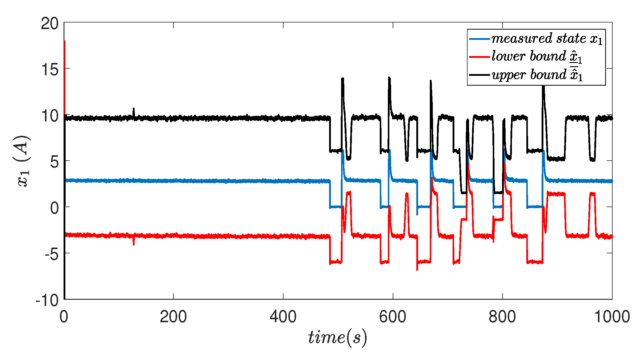
Figure 2 shows the measurement of the armature current and the limits (upper and lower) estimated by the interval observer. It can be seen in the figure that the current and limits slightly change their value in the presence of the fault.

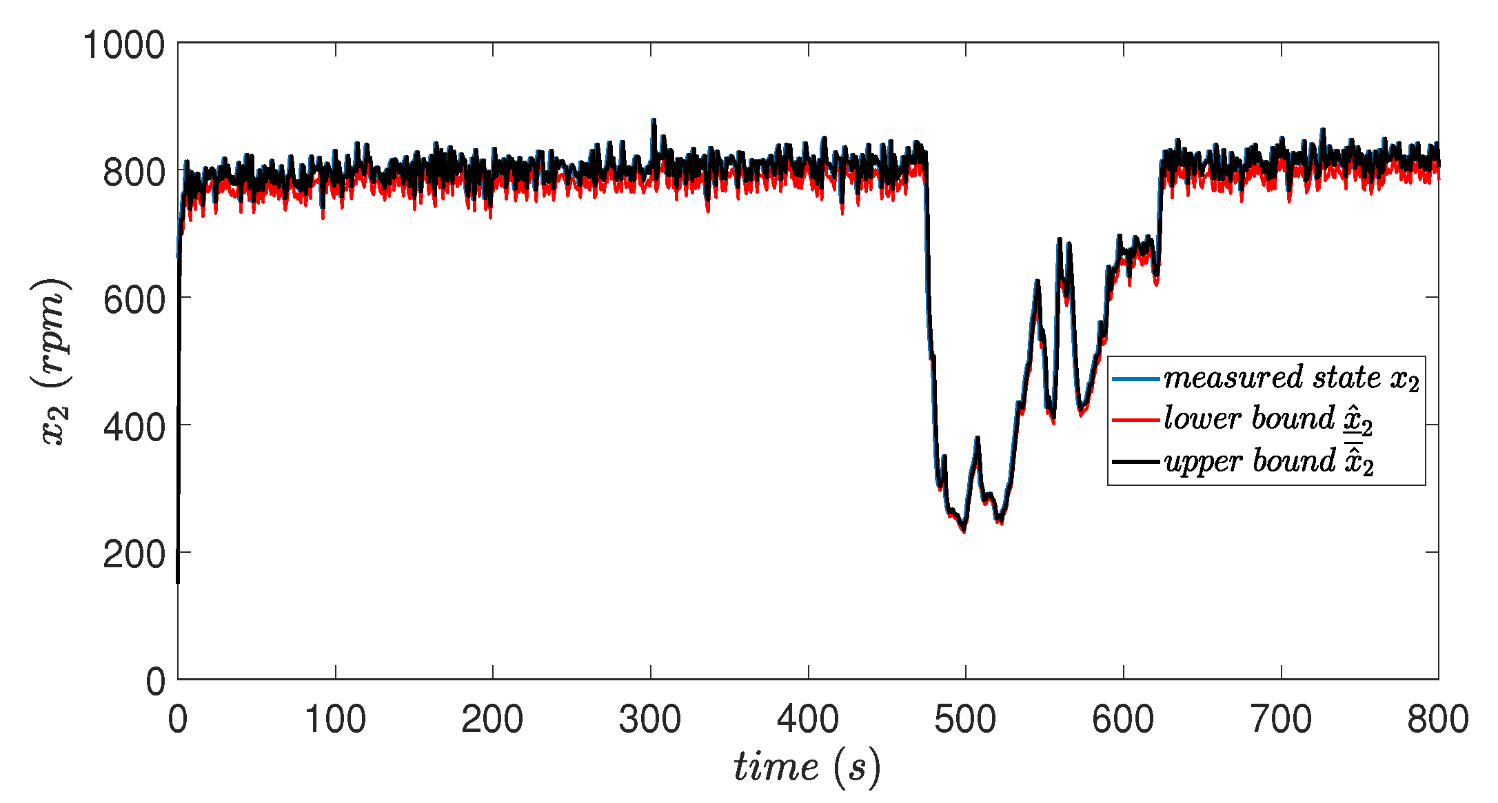
Figure 3 shows that the motor speed signal and the limits (upper and lower), estimated by the interval observer (18), present a fairly close dynamic behavior and the speed is always kept within the limits. When the fault disappears, the speed signal recovers its nominal value in approximately 120 s, with the dynamics of the motor coupled to a bearing train.

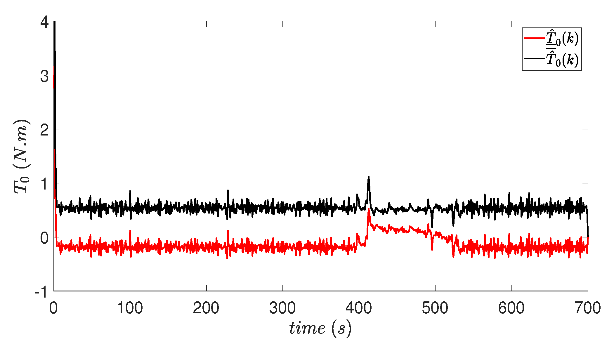
Figure 4 shows the estimated limits for the input fault, which corresponds to a change in the motor supply voltage. The limits are kept at a value of zero in the absence of failure and change their value when the fault is present.

Figure 5 and Figure 6 show the estimated values of parameters $T_0$ and $T_2$, of the parameter vector $\theta \left(k\right)$. It can be observed that these parameters remain relatively constant (around 0 and 0.5, respectively) and in the presence of the fault their values are modified. When the fault disappears, they converge again to their initial values.

Figure 7 shows the dynamic behavior of the membership functions, which meet the conditions described in Equation (33).

In the second evaluation test, the DC motor is powered with 15 V at time instant 420 s. An intermittent fault occurs in the supply voltage to the DC motor, caused by interruptions in the connection of the power supply.

Figure 8 shows the dynamic behavior of the armature current signal. Figure 9 shows the variations of the motor rotational speed signal. The current signal and the speed signal, both measurable, are maintained within their respective estimated intervals, in the presence of a fault.

Figure 10 shows the evolution of the estimated bounds for the input fault, which corresponds to change in the the voltage of the motor power supply. The limits are kept at a value centered around zero in the absence of fault and change their value when the fault is present.

Figure 11 and Figure 12 show the estimated values of parameters $T_0$ and $T_2$, of the parameter vector $\theta \left(k\right)$.

Figure 13 shows the dynamic behavior of the membership functions, which meet the conditions described in Equation (2).

5. Conclusions

A discrete-time unknown-input interval observer is proposed for a system modeled in T–S form with uncertainties. This observer allows the simultaneous estimation of unmeasured states, actuator and system faults despite disturbances and measurement noise. The structure of the proposed discrete-time T–S model has four additional terms: Three terms in the dynamic structure corresponding to the fault, disturbance and parametric uncertainty, and an additive noise term in the output (measurement noise). The conditions for the existence of the observer are formally given to guarantee the observer stability. Such conditions are derived through a Lyapunov analysis combined with a LMI formulation. The proposed discrete-time interval observer approach is experimentally evaluated by estimating the upper and lower bounds of a torque load perturbation, a friction parameter and a fault in the input voltage, in a permanent magnet DC motor.

The main advantage of the proposed T–S interval observer with respect to Kalman or Luenberger-like observers is that a great amount of nonlinear models can be transformed into the Takagi–Sugeno form, with a consequent benefit of preserving the model dynamics. This feature allows us to use this observer for a great number of nonlinear systems, in contrast with Kalman or Luenberger-like observes which requires linear or linearized systems to be implemented.

References

1. Ling, C.; Kravaris, C. State observer design for monitoring the degree of polymerization in a series of melt polycondensation reactors. Processes 2016, 4, 4. [Google Scholar] [CrossRef] [Green Version]
2. Nagy-Kiss, A.M.; Schutz, G.; Ragot, J. Parameter estimation for uncertain systems based on fault diagnosis using Takagi–Sugeno model. ISA Trans. 2015, 56, 65–74. [Google Scholar] [CrossRef] [PubMed]
3. Youssef, T.; Chadli, M.; Karimi, H.R.; Zelmat, M. Design of unknown inputs proportional integral observers for TS fuzzy models. Neurocomputing 2014, 123, 156–165. [Google Scholar] [CrossRef]
4. Peng, C.-C. Nonlinear Integral Type Observer Design for State Estimation and Unknown Input Reconstruction. Appl. Sci. 2017, 7, 67. [Google Scholar] [CrossRef] [Green Version]
5. Zhang, K.; Jiang, B.; Shi, P.; Xu, J. Fault estimation observer design for discrete-time systems in finite-frequency domain. Int. J. Robust Nonlinear Control. 2015, 25, 1379–1398. [Google Scholar] [CrossRef]
6. Van Nguyen, T.; Ha, C. Sensor Fault-Tolerant Control Design for Mini Motion Package Electro-Hydraulic Actuator. Processes 2019, 7, 89. [Google Scholar] [CrossRef] [Green Version]
7. Ifqir, S.; Ichalal, D.; Oufroukh, N.A.; Mammar, S. Robust interval observer for switched systems with unknown inputs: Application to vehicle dynamics estimation. Eur. J. Control 2018, 44, 3–14. [Google Scholar] [CrossRef]
8. Zhang, K.; Jiang, B.; Yan, X.-G.; Shen, J. Interval Sliding Mode Observer Based Incipient Sensor Fault Detection With Application to a Traction Device in China Railway High-Speed. IEEE Trans. Veh. Technol. 2019, 68, 2585–2597. [Google Scholar] [CrossRef]
9. Abadi, A.; El Amraoui, A.; Mekki, H.; Ramdani, N. Guaranteed trajectory tracking control based on interval observer for quadrotors. Int. J. Control 2019, 1–17. [Google Scholar] [CrossRef]
10. Chang, Y.-C.; Tsai, C.-T.; Lu, Y.-L. Current Control of the Permanent-Magnet Synchronous Generator Using Interval Type-2 TS Fuzzy Systems. Energies 2019, 12, 2953. [Google Scholar] [CrossRef] [Green Version]
11. Liu, F.; Li, R.; Dreglea, A. Wind Speed and Power Ultra Short-Term Robust Forecasting Based on Takagi–Sugeno Fuzzy Model. Energies 2019, 12, 3551. [Google Scholar] [CrossRef] [Green Version]
12. Lendek, Z.; Guerra, T.M.; Babuska, R.; De Schutter, B. Stability Analysis and Nonlinear Observer Design Using Takagi-Sugeno Fuzzy Models; Springer: Berlin/Heidelberg, Germany, 2011. [Google Scholar]
13. Li, J.; Wang, Z.; Shen, Y.; Wang, Y. Interval Observer Design for Discrete-Time Uncertain Takagi—Sugeno Fuzzy Systems. IEEE Trans. Fuzzy Syst. 2019, 27, 816–823. [Google Scholar] [CrossRef]
14. Rotondo, D.; Fernandez-Canti, R.M.; Tornil-Sin, S.; Blesa, J.; Puig, V. Robust fault diagnosis of proton exchange membrane fuel cells using a Takagi-Sugeno interval observer approach. Int. J. Hydrogen Energy 2016, 41, 2875–2886. [Google Scholar] [CrossRef] [Green Version]
15. Ifqir, S.; Ichalal, D.; Oufroukh, N.A.; Mammar, S. Adaptive Threshold Generation for Vehicle Fault Detection using Switched TS Interval observers. IEEE Trans. Ind. Electron. 2019. [Google Scholar] [CrossRef]
16. Ohtake, H.; Tanaka, K.; Wang, H.O. Fuzzy modeling via sector nonlinearity concept. Integr. Comput. Aided Eng. 2003, 10, 333–341. [Google Scholar] [CrossRef]
17. Rotondo, D.; Witczak, M.; Puig, V.; Nejjari, F.; Pazera, M. Robust unknown input observer for state and fault estimation in discrete-time Takagi–Sugeno systems. Int. J. Syst. Sci. 2016, 47, 3409–3424. [Google Scholar] [CrossRef] [Green Version]
18. Hui, S.; Żak, S. Observer design for systems with unknown inputs. Int. J. Appl. Math. Comput. Sci. 2005, 15, 431–446. [Google Scholar]
19. Efimov, D.; Raïssi, T.; Perruquetti, W.; Zolghadri, A. Estimation and control of discrete-time LPV systems using interval observers. In Proceedings of the 52nd IEEE Conference on Decision and Control, Florence, Italy, 10–13 December 2013; pp. 5036–5041. [Google Scholar]
20. De Oliveira, M.C.; Bernussou, J.; Geromel, J.C. A new discrete-time robust stability condition. Syst. Control Lett. 1999, 37, 261–265. [Google Scholar] [CrossRef]
21. Tuan, H.D.; Apkarian, P.; Narikiyo, T.; Yamamoto, Y. Parameterized linear matrix inequality techniques in fuzzy control system design. IEEE Trans. Fuzzy Syst. 2001, 9, 324–332. [Google Scholar] [CrossRef] [Green Version]
22. Liu, X.-Q.; Zhang, H.-Y.; Liu, J.; Yang, J. Fault detection and diagnosis of permanent-magnet DC motor based on parameter estimation and neural network. IEEE Trans. Ind. Electron. 2000, 47, 1021–1030. [Google Scholar]
Figure 1. Laboratory prototype.
Processes 08 00061 g001
Figure 2. Measurement of armature current x 1 ( k ) and estimation of interval bounds.
Processes 08 00061 g002
Figure 3. Measurement of rotational speed x 2 ( k ) and estimation of interval bounds.
Processes 08 00061 g003
Figure 4. Estimation of the bounds for the input voltage fault.
Processes 08 00061 g004
Figure 5. Estimation of T 0 ( k ) .
Processes 08 00061 g005
Figure 6. Estimation of T 2 ( k ) .
Processes 08 00061 g006
Figure 7. Membership functions.
Processes 08 00061 g007
Figure 8. Measurement of armature current x 1 ( k ) and estimation of interval bounds.
Processes 08 00061 g008
Figure 9. Measurement of rotational speed x 2 ( k ) and estimation of interval bounds.
Processes 08 00061 g009
Figure 10. Estimation of the limits of input voltage fault.
Processes 08 00061 g010
Figure 11. Upper and lower bound estimations of T 0 ( k ) .
Processes 08 00061 g011
Figure 12. Upper and lower bound estimations of T 2 ( k ) .
Processes 08 00061 g012
Figure 13. Membership functions.
Processes 08 00061 g013