Article

Economic Reliability-Aware MPC-LPV for Operational Management of Flow-Based Water Networks Including Chance-Constraints Programming

by
Fatemeh Karimi Pour
1,
Vicenç Puig
1,* and
Gabriela Cembrano
1,2
1
Automatic Control Department, Universitat Politècnica de Catalunya Institut de Robòtica i Informàtica Industrial (CSIC-UPC), C/. Llorens i Artigas 4-6, 08028 Barcelona, Spain
2
Cetaqua, Water Technology Centre, Ctra. d’Esplugues 75, Cornellà de Llobregat, 08940 Barcelona, Spain
*
Author to whom correspondence should be addressed.
Processes 2020, 8(1), 60; https://doi.org/10.3390/pr8010060
Submission received: 17 October 2019 / Revised: 15 December 2019 / Accepted: 24 December 2019 / Published: 2 January 2020
(This article belongs to the Special Issue Optimization for Control, Observation and Safety)

Abstract

:
This paper presents an economic reliability-aware model predictive control (MPC) for the management of drinking water transport networks (DWNs). The proposed controller includes a new goal to increase the system and components reliability based on a finite horizon stochastic optimization problem with joint probabilistic (chance) constraints. The proposed approach is based on a single-layer economic optimization problem with dynamic constraints. The inclusion of components and system reliability in the MPC model using an Linear Parameter Varying (LPV) modeling approach aims to maximize the availability of the system by estimating system reliability. On the other hand, the use of a LPV-MPC control approach allows the controller to consider nonlinearities in the model in a linear like way. Moreover, the resulting MPC optimization problem can be formulated as a Quadratic Programming (QP) problem at each sampling time reducing the computational burden/time compared to solving a nonlinear programming problem. The use of chance-constraint programming allows the computation of an optimal strategy with a pre-established risk acceptability levels to cope with the uncertainty of the demand forecast. Finally, the proposed approach is applied to a part of the water transport network of Barcelona for demonstrating its performance. The obtained results show that the system reliability of the DWN is maximized compared with the other approaches.

1. Introduction

The real-time control and supervision of drinking water networks (DWNs) is a field of increased interest given the environmental, economic and social impact [1]. DWNs are critical infrastructures in urban environments. These networks provide important services in modern society and maintaining the service availability is an important requirement. Therefore, reliability and resilience are important properties to be guaranteed in DWNs while being subject to constraints and continuously varying conditions of probabilistic nature [2]. DWNs are multivariate dynamic constrained systems that are described by the interconnection of several subsystems (tanks, actuators, sources, nodes and consumer sectors). Moreover, DWN optimal management is a complex challenge for water utilities that can be addressed as a multi-objective optimization problem. This problem can be solved online using a Model Predictive Control (MPC) scheme [3].
Generally, the structure of the MPC approach follows a moving horizon strategy. The control action is obtained solving an optimal control problem that provides a control action sequence in a prediction horizon that minimizes the considered control objectives and satisfies the set of constraints including the system model and physical/operational limitations. Therefore, MPC can provide suitable strategies to achieve the DWN operational control improving their performance, as it allows computing optimal control approaches ahead of time for all the pressure and flow control elements [4]. Revising the literature, different approaches can be found that show the benefits of the optimal DWN management. In [5,6,7], by optimizing a mathematical function that considers operational goals in a specific time horizon and using a model of the network dynamics and demand forecasts, optimal strategies are computed. These references also assumed predicted disturbances as defined in the model, but involve a soft constraint to penalize evacuation of water volume below a heuristic safety threshold without forcing any target regulation. Regarding optimised control strategies for managing water systems, MPC is not implemented in a classical way, as there is no reference volume to be tracked [8]. The standard MPC forces the system to follow the set point, but it does not guarantee that the system evolution toward the set points is obtained in an economic efficient way. The general aim in the operation of several process industries, as, e.g., DWNs, is the reduction of costs associated to the consumption of energy, which is not the main goal of standard MPC. For this purpose, Economic MPC (EMPC) provides a systematic method for the optimization of economic system operation [9]. The problem of optimization associated to the EMPC strategy aims at obtaining a family of optimal set points considering economic efficiency rather than aiming that the controlled system reach a certain set point [9].
The use of control strategies that take into account the system and component reliability that guarantee the quality of service is necessary. The health monitoring of the actuator and system should be considered for increasing the system reliability, minimising the fault appearance and reducing the operational costs. In the later stages, system reliability in the process of control system has been considered using a Prognosis and Health Management (PHM) framework. This is because reliability is a standard method for evaluating how long the system will achieve its function without malfunctions. Moreover, it can be used to predict future damages in the system according to the health state of its components [10].
In the past few years, the problems of system reliability and actuator lifetime in service has received considerable interest for the researcher community. In [11], to decrease the maintenance cost, the actuator lifetime is regarded as a controlled parameter that is considered as additional goal when using a linear quadratic optimal controller. On the other side, MPC predicts the suitable control actions to obtain optimal performance according to multi-objective cost functions and physical constraints, and therefore it can be considered as a suitable approach for developing health-aware control schemes. An MPC strategy based on distributing the loads among redundant actuators is introduced in [12], while forcing constraints to guarantee that the accumulated actuator degradation will not arrive at the unsafe level at the end of the prediction horizon. In [13], the authors proposed a health-aware MPC controller that incorporates a fatigue-based prognosis into MPC to minimize the component damage. Most of the other methods that consider component health and system reliability management stand within the structure of fault-tolerant control or in the area of preservation scheduling see, e.g., Gallestey et al. [14], Khelassi et al. [15], Salazar et al. [16] and references therein. However, none of these methods consider uncertainty.
The reliability is the system’s ability (or component) to carry out its expected functions. The reliability of DWN is influenced by different conditions such as the capacity and the quality of the water accessible at the sources and the pump/pipe failure rates [17,18]. In most of the works, the actuator reliability is assumed that follows an exponential distribution that varies with the control action [19]. The system reliability is characterised according to the interdependence topology based on the combining of each actuator reliability. Subsequently, the system reliability has a demonstrative relationship with the control input that leads to a nonlinear mathematical model. In several studies, this is achieved by including a damage index in the optimization problem and establishing a trade-off by weight tuning [20] or by imposing constraints with respect to the actuator reliability [17]. However, considering the reliability at the actuator level not at the system level is the main drawback of the previous methods; otherwise, it leads to the use of nonlinear MPC according to nonlinearity of the resulting constraints. Generally, Economic Nonlinear MPC (ENMPC) implies a high computational cost and, the existing gradient-based numerical algorithms do not certify that the obtained solution corresponds to the global one because of the non-convexity of the associated optimization problem. Transforming the nonlinear optimization problem into a quadratic problem through a linearisation method is one way of addressing the non-convexity problem and guaranteeing a unique optimum. In this way, the system is modelled by an incremental model because the model has to be linearised at each iteration. This approach has been improved by means of of the use Linear Parameter Varying (LPV) models that do not require linearisation [21]. The LPV models can describe both nonlinear phenomena and time-varying that can be estimated/measured online.
Another weakness of previous approaches combining reliability analysis and MPC is the conservatism of the resulting control strategies, which affects negatively the efficient DWN operation. Furthermore, in real applications, the assumption of bounded disturbances in real applications is not always satisfied. Thus, constraint violations can not be avoided because of the appearance of faults, unexpected events, etc. A more realistic representation of uncertainty is based on using the stochastic approach that leads to less conservative control methods by incorporating explicit disturbance models in the control design and by converting hard constraints into probabilistic constraints. The stochastic approach is a sophisticated theory in the field of optimization, but a revived consideration has been provided to the stochastic programming methods as powerful tools for the design of controllers, leading to the stochastic MPC, which has a particular alternative called chance-constrained MPC (CC-MPC) [22,23]. The stochastic control approach that represents robustness in terms of probabilistic (chance) constraints, which need that the probability of violation of any operational condition or physical constraint is under a designated value. By placing this value suitably, the user/operator can obtained the desired trade-off between robustness and performance. For related works that proposed the CC-MPC approach in water networks the reader is referred to [24,25]. Some economic-oriented controller that consider the reliability issue has been proposed [20], but without considering reliability at the system level and probabilistic constraints based on the reliability of the system.
The aim of this paper is to include in an EMPC strategy for DWN an additional objective that takes into account PHM information obtained by the online evaluation of the system reliability. The system reliability is incorporated into the control algorithm by using an augmented model that includes both the reliability and DWN models. As the reliability model of the whole DWN is nonlinear, its model is expressed as an LPV model such that at each time instant the varying parameters are updated according to the value of the scheduling variables. This allows to solve the optimization MPC problem associated to the health-aware approach using quadratic programming instead of nonlinear programming. Considering the probabilistic nature of system reliability, it is included in the MPC optimization problem in the form probabilistic constraints as the demands (disturbances) using the chance constraints programming paradigm. The resulting control inputs obtained by the proposed health-aware MPC approach are able to achieve the economic control objectives and simultaneous to increase the lifespan and reliability of the system components.
Chance-constraints programming allow to determine an optimal strategy by establishing the desired level of infeasibility and system reliability. Moreover, it allows considering the system reliability, which is assessed online using an LPV-MPC strategy; representing the main contribution of this paper. The second contribution is to propose an advanced health-aware LPV-MPC approach that formulates a quadratic optimization problem taking into account the functional dependency of scheduling variables and state vector. This approach avoids the use of nonlinear optimization. Moreover, it uses chance constraints programming to manage dynamically designate safety stocks in flow-based networks to satisfy nonstationary flow demands and system reliability.
The structure of the paper is as follows. The control-oriented model considered for DWN when considering the transportation layer is introduced in Section 2. Section 3 presents the chance-constraints programming and the way to use it into the MPC controller. The system reliability modeling and the relationship between reliability and chance constricted are described in Section 4. In Section 5, the economic reliability-aware MPC-LPV including chance-constraints programming is provided. The results of the application of the proposed control strategy to the DWN network using the proposed case study are analyzed and summarized in Section 6. Finally, the conclusions and research future paths are presented in Section 7.
Notation: Throughout this paper R , R + , R n , R m × n indicate the field of real numbers, the set of non-negative real numbers, the set of column real vectors of length n, and the set of m by n real matrices, respectively. Equivalently, I + presents the set of non-negative integer numbers including zero. Define the set I [ a , b ] : = { x I + | a x b } for some a , b I + and I c : = { x I + | x c } for some c I + . The operator ⊕ is direct sum of matrices (block diagonal concatenation). Furthermore, . denotes the spectral norm for matrices and | | . | | 2 is the squared 2-norm symbol. The superscript represents the transpose and operators < , , = , > , indicate element-wise relations of vectors.

2. EMPC for Transport Water Networks

2.1. Control-Oriented Model

In the literature, several control-oriented models for DWNs can be found depending if the transportation or distribution layer is considered. (see, e.g., in [26,27]). In this paper, a flow-based control-oriented modeling approach is considered following [6,28] since the transportation layer is considered. A DWN is composed by pipes, water tanks, pumping stations, and valves used for consumer water supply. To derive the control oriented-model, the state vector x R n x is defined to represent the tank volumes. The vector u R n u of controlled inputs is associated to the flow rates through the actuators (pumps and valves) of the network, and the vector d m R n d of disturbances (demands) as the collection of flow rates required by the consumers at demand nodes. By means fo the flow–mass balance relations in the tanks and nodes, a discrete-time model based on linear differential algebraic equations (DAEs) for all time instant k Z 0 can be formulated for a given DWN as follows,
x ( k + 1 ) = A x ( k ) + B u ( k ) + B d d m ( k ) ,
0 = E u u ( k ) + E d d m ( k ) ,
where difference Equation (1a) model the dynamics of the storage tanks, whereas the algebraic relations (1b) describe the mass balance at junction nodes. A R n x × n x , B R n x × n u , B d R n x × n d , E u R n d × n u , E d R n d × n d , and C R n y × n x are time-invariant matrices of that depends on the network topology. The system is subject to physical input and state constraints provided by convex and closed polytopic sets defined as
x ( k ) X : = { x R n x | G x g } ,
u ( k ) U : = { u R n u | H u h } ,
for all k Z 0 , where G R m x × n x , g R m x , H R m u × n u , and h R m u are vectors/matrices collecting the system constraints, signifying m u Z 0 and m x Z 0 , the number of input and state constraints, respectively. Concerning the operation of the considered flow-based networks, the following assumptions are considered in this paper.
Assumption A1.
The demands in d m ( k ) and the states in x ( k ) are observable at each time instant k Z 0 , also the pair ( A , B ) is stabilizable.
Assumption A2.
The demand realizations at the current time instant k Z 0 can be represented as
d m ( k ) = d ¯ m ( k ) + d ˜ m ( k ) ,
where d ¯ m ( k ) is the vector of expected disturbances that can be forecast, and d ˜ m ( k ) is the vector of probabilistic independent forecasting errors with nonstationary uncertainty and a known (or approximated) quasi-concave probability distribution D 0 , ( d ¯ m , ( j ) ( k ) ) . Consequently, each j-th row of d m ( k ) is described by an stochastic variable d ¯ m , ( j ) ( k ) D ( j ) d ¯ m , ( j ) ( k ) , ( d ˜ m , ( j ) ( k ) ) , where d ¯ m , ( j ) ( k ) represents the mean and  ( d ˜ m , ( j ) ( k ) ) the variance.

2.2. EMPC Formulation

Computing the input commands ahead of time, to obtain the optimal performance of the network according to a set of control goals, is the purpose of applying MPC techniques for managing water transportation networks [1]. The control goal is to minimize a convex stage cost function : Z 0 × X × U R 0 , which might carry any functional relationship with the economics of the system operation. Therefore, the control aim can be expressed for minimization of a convex multi-objective cost function, which involves three functional objects for managing the DWN with different types:
  • Economic objective: Minimizing water production and transport costs while providing the demanded volume.
  • Safety objective: The safety volumes in the tanks are preserved guaranteeing, up to some level, the water supply under connected variations in the demand.
  • Smoothness objective: For avoiding overpressures in pipes and damage in actuators, the actuators are managed based on the smooth control actions.

2.2.1. Economic Cost Minimization

Minimizing the economical costs that include water production and electrical costs related to pumping is the main control objective of the DWN. Transporting drinking water to proper elevation levels by the network involves significant electricity costs due to pumping. Therefore, the cost function related to this objective can be expressed as
e ( k ) α ( k ) W e u ( k ) ,
where α ( k ) ( α 1 + α 2 ( k ) ) R n u , α 1 R n u denotes a fixed water production costs that related to the water treatments, and α 2 R n u corresponds to a time-varying water cost associated to pumping that varies in each time instant k with respect to the dynamic electricity tariff. W e indicates the weighting term that allows to prioritize the economic control objective in the complete objective function.

2.2.2. Safety Management

To preserve water stocks in spite of unexpected changes in the water demands, an appropriate safety storage level for each tank is required to be guaranteed. This goal can be formulated in the following manner,
s ( k ) x ( k ) - x s 2 , i f   x ( k ) x s 0 ,   o t h e r w i s e
where x s indicates the tanks safety levels. This piecewise linear formulation can be avoided by considering that the safety cost function can be expressed through a soft constraint by using a slack variable ξ , which is introduced to retain feasibility of the optimization problem and minimized
s ( k ) ξ ( k ) W s ξ ( k ) ,
and the soft constraint is defined as
x ( k ) x s - ξ ( k ) ,
and W s is diagonal positive definite matrix that allows to prioritize this objective in the complete objective function.

2.2.3. Control Action Smoothness

Pumps and valves are the considered actuators in a DWN. Therefore, the control actions obtained by the MPC controller must be smooth for the purpose of preserving the component lifetime. To achieve the smoothing effect, the variation of the control actions among two consecutive time instants is penalized as follows,
Δ u ( k ) Δ u ( k ) W Δ u Δ u ( k ) ,
where Δ u ( k ) u ( k ) - u ( k - 1 ) , and  W Δ u is a weighting matrix that allows prioritizing this objective in the complete objective function.

2.2.4. EMPC Optimization Problem Formulation

The EMPC strategy can be implemented by solving a finite-horizon optimization problem over a prediction horizon N p , where the multi-objective cost function is minimized subject to the prediction model and a set of system constraints. According to the network model (1), the MPC controller design is based on minimizing the following cost function in the prediction horizon N p ,
J = l = 0 N p ( e ( l | k ) + s ( l | k ) + Δ u ( l | k ) ) .
where at each time instant, the following optimization problem is solved online.
min u ( k ) , x ( k ) , ξ ( k ) J ( u ( k ) , x ( k ) , ξ ( k ) ) ,
subject to:
x ( l + 1 | k ) = A x ( l | k ) + B u ( l | k ) + B d d m ( l | k ) , l = 0 , , N p - 1 ( l0 b ) 0 = E u u ( l | k ) + E d d m ( k ) , l = 0 , , N p - 1 ( l0 c ) x ( l | k ) x s - ξ ( l | k ) , l = 1 , , N p ( l0 d ) u ( l | k ) U , l = 0 , , N p - 1 ( l0 e ) x ( l | k ) , X , l = 1 , , N p ( l0 f ) ξ ( l | k ) 0 , l = 0 , , N p ( l0 g ) x ( 0 | k ) = x ( k ) , ( l0 h )
The optimal control actions sequence u ( k ) = { u ( l | k ) } l Z [ 0 , N p - 1 ] , x ( k ) = { x ( l | k ) } l Z [ 1 , N p ] , and ξ ( k ) = { x i ( l | k ) } l Z [ 1 , N p ] are obtained online. Considering the receding horizon philosophy [3], the procedure is based on solving the optimization problem (10a) from the current time instant k to k + N p by using x ( 0 | k ) as the initial condition that is computed from measurements (or state estimation) at time k. Then, by applying the first value u ( 0 | k ) from the optimal input sequence u ( k ) to the system, the procedure goes to the next time instant. To calculate u ( 0 | k + 1 ) at time k + 1 , the optimization problem (10a) is solved from k + 1 to k + 1 + N p , and initial states x ( 0 | 1 + k ) from measurements (or state estimation) are updated at time k + 1 . The same method is iterated for the following time instants.

3. Chance-Constrained Model Predictive Control

If the stochastic nature of disturbances (demands) and reliability of components of the system is not explicitly considered, an optimal solution of (10) satisfying all constraints can not be found in real scenarios. Therefore, to guarantee feasibility of the optimization problem (10), it is appropriate to relax the original constraints that involve stochastic elements with probabilistic statements in the form of chance constraints. In this manner, the constraints are needed to be satisfied with predefined risk levels to manage the uncertainty and component reliability of the system. Chance-constrained programming is a technique of stochastic programming dealing with constraints of the general form as
P [ f ( v , ζ ) 0 ] 1 - δ ζ ,
where P indicates the probability operator, v R n v is the decision vector, ζ R n ζ a random variable, and f : R n v × R n ζ R n c a constraint mapping. The level δ ζ ( 0 , 1 ) is user given and defines the preference for safety of the decision v. The constraint (11) means that we wish to take a decision v that satisfies the n c -dimensional random inequality system f ( v , ζ ) 0 with high enough probability. As demonstrated in [29], if f ( . , . ) is jointly convex in ( v , ζ ) and Φ P [ . ] is quasi-concave, then the feasible set
Ψ ( δ ζ ) { v | P [ f ( v , ζ ) 0 ] 1 - δ ζ }
is convex for all δ ζ ( 0 , 1 ) . All chance-constrained models need prior knowledge of the acceptable risk δ ζ connected with the constraints. A lower risk acceptability proposes a harder constraint. In general, joint chance constraints lack from analytic expressions because of the involving multivariate probability distribution [30]. In this paper, by following the results in [30,31], a uniform distribution of the joint risk is approximated by upper bounding the joint constraint and assuming a similar distribution of the joint risk among a set of individual chance constraints are transformed inside equivalent deterministic constraints.
Consider the general joint chance constraint (11), and define f ( v , ζ ) ζ F v with F R ζ × n v . Therefore, the additive stochastic element is separable and the following chance constraint is achieved,
P [ ζ F v ] 1 - δ ζ .
Then, by rewiring ω F v , for any duple ( ζ , ω ) , it follows that
Φ ζ ( ω ) = P [ { ζ 1 ω 1 , . . . , ζ n c ω n c } ] .
Describing the events C i { ζ i ω i } , i Z 1 n c (as e.g., faults in the actuators or unexpected changes in the demand), it follows that
Φ ζ ( ω ) = P [ C i . . . C n c ] .
Indicating the complements of the events C i by C i c { ζ i > ω i } , and it is obvious from probability theory that
C 1 . . . C n = ( C 1 c . . . C n c c ) c ,
and consequently
Φ ζ ( ω ) = P [ C i . . . C n c ] ( l7 a ) = P [ ( C 1 c . . . C n c c ) c ] ( l7 b ) = 1 P [ ( C 1 c . . . C n c c ) c ] 1 δ ζ . ( l7 c )
By using the union bound, the Boole inequality let to bound the result in (17a), declaring that for a countable set of events, the probability that at least one event occurs is not higher than the sum of the individual probabilities [32], such that
P i = 1 n c C i i = 1 n c P [ C i ] ,
and, by applying (18) to (17a), it yields to
i = 1 n c P [ C i c ] δ ζ i = 1 n c ( 1 P [ C i ] ) δ ζ .
Then, a set of constraints rises from previous results as sufficient conditions to enforce the joint chance constraint (13), by allotting the joint risk δ ζ in n c separate risks δ ζ , i , i Z i n c . These constraints are described as follows,
        P [ C i ] 1 - δ ζ , i , i Z 1 n c
i = 1 n c δ ζ , i δ ζ ,
0 δ ζ , i 1 ,
where (20a) produces the set of n c effective individual chance constraints, which bounds the probability that each inequality of the receding horizon problem could not be satisfied. Moreover, (20b) and (20c) are conditions forced to bound the new single risks in such a way that the joint risk bound is not breached. Each solution that satisfies the aforesaid constraints is guaranteed to provide (13).
According to the satisfaction of each individual constraint is an event C i , i Z i n c . A joint chance constraint needs that the connection of all the individual constraints is satisfied with the wanted probability level, such as
P i = 1 n c C i 1 - δ ζ .
Considering that each individual constraint is probabilistically dependent, the level of conservatism can be derived by using the inclusion–exclusion principle for the union of finite events, C i , i Z 1 n c , which proves the following equality,
P i = 1 n c C i = i = 1 n c P [ C i ] 1 i < j n c P C i C j + 1 i < j < k n c P C i C j C k + ( 1 ) n c - 1 P i = 1 n c C i .
Note that by considering as an event a fault in an actuator, it can be observed that Equation (22) has a similar as formulation as the one used for evaluating the system reliability based on the component reliability.
In a DWN, the constraints come from models (10b) and (10c) that can be formulated as chance constraints statements taking into account the probabilities associated to the component reliability. Considering only faults in actuators, the reliability of the system is related to the system inputs u i ( k ) . Therefore, (11) can be formulated in case of the actuators as follows,
P [ f ( u i ( k ) , ζ i ( k ) ) 0 ] 1 - δ ζ i ,
where ζ ( k ) { 0 , 1 } is a stochastic variable which considers if the actuator is one of two states { U n v a i l a b l e , A v a i l a b l e } (or { 0 , 1 } ) defined as follows,
ζ i ( k ) = 1 , R i ( k ) > 0 0 , R i ( k ) = 0 .
where R i ( k ) is the actuator reliability. In the case that ζ i ( k ) = 1 , the input u i ( k ) associated to the i-th actuator is bounded by (2b); otherwise, an additional constraint setting u i ( k ) = 0 should be included. Furthermore, to determine the reliability associated to the system that associates a probability to the system model constraint (1), the joint-chance constraint probability calculation (22) should be used leading to the following probabilistic formulation for the MPC optimization problem (10),
min u ( k ) , x ( k ) , ξ ( k ) J ( u ( k ) , x ( k ) , ξ ( k ) ) ,
subject to
P [ A x ( l | k ) + B ( ζ i ) u ( l | k ) + B d d m ( l | k ) , ( 25 b ) E u ( ζ i ) u ( l | k ) + E d d m ( k ) ] 1 - δ , l = 0 , , N p - 1 ( 25 c ) x ( l | k ) x s - ξ ( l | k ) , l = 1 , , N p ( 25 d ) u ( l | k ) U , l = 0 , , N p - 1 ( 25 e ) x ( l | k ) , X , l = 1 , , N p ( 25 f ) ξ ( l | k ) 0 , l = 0 , , N p ( 25 g ) x ( 0 | k ) = x ( k ) . ( 25 h )
The main difficulty in solving this stochastic problem using chance constraints is that at each time iteration, the probabilities associated to the system reliability should be updated taking into account the value of the optimal control actions u i . In the following section, a solution procedure is proposed to solve this problem.

4. Augmenting Network Model with the Reliability Model

As discussed in the introduction, one of the contributions of this work is to integrate the information about system health in the MPC controller by using the reliability approach. In the following, a procedure to derive the reliability model of the DWN is presented, considering that faults can only occur in the actuators.

4.1. Reliability Model

In the literature, different types of distributions have been considered to characterize the evolution of the reliability with time. The most commonly used are exponential, normal, log-normal, and Weibull distributions [33]. Here, the exponential function is considered.
First, define the concept of failure rate which is important to obtain reliability. The general explanation of failure rate, indicated by λ is presented as the fraction of the density of the stochastic lifetime to the remainder function (i.e., conditional probability). Particularly, systems are designed to work under different load values. According to [33], the load firmly affects the component failure rate. Therefore, for presenting system reliability evaluation should be considered the load versus failure rate relationship. A significant amount of literature has been produced to include the impact of the load level in the reliability estimation [33]. In this paper, actuator failure rates under various load levels are considering in function of the applied control input. The following exponential laws is the most widely used relationship to characterize the variation of the actuator fault rates with the load
λ i = λ i 0 e x p β i u i ( k ) , i = 1 , 2 , , m
where λ i 0 represents the baseline failure rate (nominal failure rate) and u i ( k ) is the control action a time k for the i-th actuator. β i is a constant parameter that depends on the actuator characteristics.
Accordingly to the failure rate definition, reliability of a system or component can be described as follows
Definition 1.
Reliability is determined as the probability that a system (or component) will perform their functioning satisfactorily for a certain period of time subject to operating conditions [34].
From the mathematical point of view, reliability R ( t ) is defined as the probability of the successful operation of a system in the intervening period from time 0 to time t:
R ( t ) = P ( T > t ) , t 0
where T is a stochastic variable that describes time until failure. Furthermore, the unreliability of system (or a component) is represented as follows.
Definition 2.
The unreliability F ( t ) is determined as the probability that the component or system encounters the first failure or has failed one or more times among the time interval 0 to time t.
Considering the system (or component) is always in one of the two states introduced in Equation (24), the following relationship is provided,
F ( t ) + R ( t ) = 1 .
The reliability of a component R 0 ( t ) in the useful life period can be specified at a certain time t by a starting point. Accordingly, R 0 , i ( t ) will denote the i-th actuator reliability determined considering nominal operating conditions
R 0 , i ( t ) = e x p - λ i 0 t , i = 1 , 2 , , m
Therefore, the components reliability of a system with the i-th components can be computed by exploiting the exponential function and the baseline reliability level R 0 , j as follows,
R i ( t ) = R 0 , i e x p - 0 k λ i ( s ) d s , i = 1 , 2 , , m
In discrete-time, Equation (30) can be rewritten as
R i ( k + 1 ) = R 0 , i ( k ) + e x p - T s s = 0 k + 1 λ i ( s ) , i = 1 , 2 , , m
where λ i ( s ) is the failure rate that is acquired from the i-th component under varying load levels u i and T s is the sampling time.

4.2. Overall Reliability

The system lifespan can be determined by the reliability of the overall system that is denoted as R g ( k ) . This reliability is obtained based on the computation of the reliabilities of elementary components (or subsystems). Therefore, R g ( k ) is influenced by the configuration of the actuator that can be computed from the combination of parallel and/or series of subsystems (or components) [35]. However, there are several engineering systems that not attending the parallel, series, or connection of parallel and series structures. To manage the more complex situations, a graph model can be used to determine if the component successful path existence can be identified to determine whether the system is working correctly. A path for the graph network is a set of components, in such a way that the system will succeed just when all the components are successful in that set. A minimal path P s is a set of components that relates to it, but the elimination any one of the components will create the set not to be a successful path [35]. Therefore, the overall system reliability R g ( k ) can be counted as
R g ( k ) = 1 - j = 1 s 1 - i P s , j R i ( k ) ,
where j = 1 , , s is minimal paths number. As mentioned in previous section, there is an indirect relationship between conservatism of probability and the overall system reliability. In fact, the formula obtained for overall reliability system (Equation (32)) can be obtained from Equation (22).

4.3. System Reliability Modeling

Aiming to include reliability in the MPC model, a transformation is needed allowing to estimate reliability in a LPV framework. The considered transformation relies on applying the logarithm to (32). Then, Equation (32) can be rewritten as follows,
log ( Q g ( k ) ) = log j = 1 s 1 - i p s , j R i ( k ) ,
and by introducing an change of variable
z j ( k ) = 1 - i p s , j R i ( k ) ,
Equation (33) can be expressed as
log ( Q g ( k ) ) = i p s , j s log ( z j ( k ) ) .
Considering (34), the log ( z j ( k ) ) can be determined as
log ( z j ( k ) ) = log ( z j ( k ) ) log ( 1 - z j ( k ) ) i p s , j log R i ( k ) .
Afterward, by renaming β j ( k ) = log ( z j ( k ) ) log ( 1 - z j ( k ) ) in (36), (33) can be rewritten as
log ( Q g ( k ) ) = i p s , j s β j ( k ) i p s , j log R i ( k ) .
Finally, the system unreliability can be computed from the unreliability of the baseline system
log ( Q g ( k + 1 ) ) = log ( Q g ( k ) ) + i p s , j s β j ( k ) i p s , j log R i ( k ) .

5. Economic Reliability-Aware MPC-LPV Using Chance-Constraints

5.1. Economic Reliability Aware MPC-LPV

In this section, the integration of reliability model in the MPC controller augmenting the DWN model is proposed. As previously discussed, the reliability of the DWN can be determined by employing the control input. Thus, a new objective can be included in the MPC controller that aims to preserve the system reliability additionally to consider the reliability model (38). Figure 1 summarizes the procedure to obtain the augmented control model from the dynamic model of DWN by obtaining the reliability model using Equation (32) or equivalently Equation (22).
By following this procedure, the augmented MPC model can be formulated as follows,
x g ( k + 1 ) = A g x r ( k ) + B g u ( k ) + B d , g d m ( k ) , y g ( k ) = C g x ( k ) ,
where the state and output vector are defined by x g = [ x , log ( Q g ) , log ( R 1 ) , , log ( R i ) ] T and y g = [ y , log ( Q g ) ] T , respectively. The augmented matrices are defined as
A g = A 0 n x × n i + 1 0 1 × n x 1 i p s , j s β j ( k ) 0 n i × n x I n i × n i , B g = B n u × n u 0 - λ i × I n i × n i , B d , g = B d , n u × n u 0 n i + 1 × n B d , C g = C 0 0 0 0 1 0 0 .
Considering the control action u i ( k ) as the scheduling variable related to each actuator and state in the augmented MPC model, it can be considered (39) as an LPV model. The model (39) cannot be assessed before solving the optimization problem (10), due to the future state sequence is unknown and cannot be determined. In reality, x ( l | k ) depends on the future control inputs u ( k ) , and also on the future scheduling parameters, thus LPV model can not instantiated offline but instead should be evaluated online at each time instant k. In this way, the MPC optimization problem (10) can be formulated as a QP problem by using an estimation of scheduling variables, θ ^ instead of utilizing θ . That means the scheduling variables in the prediction horizon are estimated using the values from the previous MPC iteration and applied to update the model matrices of the MPC controller. Indeed, the control input sequence is utilized to change the model matrices used in the prediction horizon. Therefore, the predicted parameters and sequence of states are obtained from the optimal control sequence u ( k ) , such as
x ˜ ( k ) = x ( l + 1 | k ) x ( l + 2 | k ) x ( N p | k ) R N p , n x , Θ = θ ^ ( l | k ) θ ^ ( l + 1 | k ) θ ^ ( N p - 1 | k ) R N p , n θ .
The vector Θ ( k ) includes parameters from time k to k + N p - 1 while the state prediction is considered for time k + 1 to k + N p . Thus, by a small abuse of notation, φ is defined as Θ ( k ) = φ ( [ x T ( k ) x ˜ T ( k ) ] , u ( k ) ) . The vector Θ ( k ) consists of parameters from time k to k + N p - 1 , whereas the state prediction is performed for time k + 1 to k + N p .
Therefore, using Equation (41), the predicted states can be directly expressed as follows,
x ˜ ( k ) = A ( Θ ( k ) ) x ( k ) + B ( Θ ( k ) ) u ( k ) + B r , d d m ( k ) ,
where A R n x × n x and B R n x × n u are provided by Equations (43) and (44).
A ( Θ ( k ) ) = I A ( θ ^ ( k ) ) A ( θ ^ ( k + 1 ) ) A ( θ ^ ( k ) ) A ( θ ^ ( k + N p - 1 ) ) A ( θ ^ ( k + N p - 2 ) ) A ( θ ^ ( k ) ) ,
and
B ( Θ ( k ) ) = 0 0 0 0 B ( θ ^ ( k ) ) 0 0 0 A ( θ ^ ( k + 1 ) ) B ( θ ^ ( k ) ) B ( θ ^ ( k + 1 ) ) 0 0 A ( θ ^ k + N p - 1 ) A ( θ ^ ( k + 1 ) ) B ( θ ^ ( k ) ) A ( θ ^ k + N p - 1 ) A ( θ ^ ( k + 2 ) ) B ( θ ^ ( k + 1 ) ) B ( θ ^ k + N p - 1 ) ) 0 .
By exploiting Equation (42), and new weighting matrices w 1 ˜ = d i a g N p ( w 1 ) , and w 2 ˜ = d i a g N p ( w 2 ) , the cost function (9) with the new additional objective that aims to increase the system reliability can be revised in vector form as follows,
min u ( k ) , ξ ( k ) , x ( k ) Q g ( k ) l = 0 N p [ e ( l | k ) + s ( l | k ) + Δ u ( l | k ) - R g ( l | k ) ] ,
subject to
x ˜ ( k ) = A ( Θ ( k ) ) x ( k ) + B ( Θ ( k ) ) u ( k ) + B r , d d m ( k ) , ( 45 b ) 0 = E u u ( l | k ) + E d d m ( k ) , ( 45 c ) x ( l + 1 | k ) x s - ξ ( l | k ) ( 45 d ) log Q g ( l + 1 | k ) = x ˜ n x + 1 ( l | k ) ( 45 e ) u ( l | k ) U , l = 0 , , N p - 1 ( 45 f ) x ( l | k ) , X , l = 1 , , N p ( 45 g ) ξ ( l | k ) 0 , l = 0 , , N p ( 45 h ) x ( 0 | k ) = x ( k ) , ( 45 i )
where R g ( k ) Q g w 3 Q g is an additional objective including the weight w 3 into the controller cost function to improve the system reliability. The optimization problem is solved as a QP problem according to that the predicted states Θ ( k ) in (42) are linear with respect to control inputs u ( k ) , which is considerably further easier than solving a nonlinear optimization problem. To clarify the proposed approach, Algorithm 1 is presented.
Algorithm 1 LPV-based MPC strategy
1:
k 0
2:
repeat
3:
i 0
4:
if k = 1 then
5:
 To solve the optimization problem (45a), where θ ( 0 | k ) θ ( 1 | k ) θ ( 2 | k ) ≃ ... ≃ θ ( N p - 1 | k )
6:
 Calculate Θ ( k ) by using x ˜ ( k ) and u ( k )
7:
else
8:
 Determine Θ ( k ) = { θ ^ ( i | k ) } i = 0 N p - 1 where θ ^ ( i | k ) = ψ ( x ( i | k - 1 + 1 ) , u ( i | k - 1 ) ) ,
9:
 Solve the optimization problem (45a)
10:
 Compute x ˜ ( k ) and u ( k ) ,
11:
i i + 1
12:
end if
13:
Apply first element of the input sequence to the plant
14:
Define Θ 0 ( k + 1 ) = ψ ( x ˜ 1 ( k ) , u 0 ( k ) )
15:
k k + 1
16:
until end

5.2. Including Demand Uncertainty Using Chance Constraints

According to the stochastic nature of water demands, the DWN prediction model includes exogenous additive uncertainties. Therefore, the constraint’s satisfaction (10) cannot be guaranteed, unless uncertainty it is not explicitly considering in some way. Therefore, the original constraints that include stochastic elements (2a) will formulated by means of probabilistic statements using the chance constraints framework (11). Considering this framework introduced in Section 3, and the form of state constraint set X , the form of a state joint chance constraint is described as
P [ G ( r ) x g ( r ) , r Z [ 1 , m x ] ] 1 - δ x ,
where δ x ( 0 , 1 ) is the risk acceptability level of constraint violation for the states, and G ( r ) and g ( r ) indicate the r-th row of G and g, respectively. This entails that all rows r have to be jointly satisfied with the probability 1 - δ x . Also, the form of a state individual chance constraint is described as
P [ G ( r ) x g ( r ) , ] 1 - δ x , r Z [ 1 , m x ]
which requires that each r-th row of the inequality has to be satisfied individually with the respective probability 1 - δ x , r , where δ x , j ( 0 , 1 ) . Then, according to Equation (20), the state constraints can be described as follows,
P [ G ( r ) x g ( r ) ] 1 - δ x , r , r Z [ 1 , m x ] ( 48 a ) r = 1 m x δ x , r δ x , ( 48 b ) 0 δ x , r 1 , ( 48 c )
and, as recommended in [31], specifying a constant and equal value of risk to each individual constraint, that is, δ x , r = δ x / m x for all r Z [ 1 , m x ] , then (48b) and (48c) are obtained.
By considering a known (or approximated) quasi-concave probabilistic distribution function for the stochastic disturbance in the dynamic model (1), it yields to
P [ G ( r ) x ( k + 1 ) g ( r ) ] 1 - δ x , r F G ( r ) B d d m ( k ) ( g ( r ) - G ( r ) ( A x ( k ) + B u ( k ) ) ) 1 - δ x , r G ( r ) ( A x ( k ) + B u ( k ) ) g ( r ) - F G ( r ) B d d m ( k ) - 1 ( 1 - δ x , r ) ,
for all r Z [ 1 , m x ] , where F G ( r ) B d d m ( k ) ( . ) and F G ( r ) B d d m ( k ) - 1 ( . ) are the cumulative distribution and the left-quantile function of G ( r ) B d d m ( k ) , respectively. The use of chance constraints allows to guarantee a safety stock at each storage node of a flow-based network for decreasing the probability of stock-outs due to demand uncertainty. In this way, according to Equation (48a), the safety stocks are optimally assigned and designed by the constraint back-off effect due to the term F G ( r ) B d d m ( k ) ( 1 - δ x , r ) in Equation (46). Therefore, the original state constraint set X is adjusted by the effect of the m x deterministic equivalents in (49) and substituted by the stochastic feasibility set provided by
X s ( k ) : = { x ( k ) R n x | u ( k ) U , such that G ( r ) ( A x ( k ) + B u ( k ) ) g ( r ) - F G ( r ) B d d m ( k ) - 1 ( 1 - δ x , r ) r Z 1 , m x and E u u ( k ) + E d d ¯ ( k ) = 0 } ,
where d ¯ ( k ) = E [ d m ] is the first moment of d m for all k Z 0 0 . The set X s ( k ) is convex when non-empty for all δ x , r ( 0 , 1 ) in most distribution functions, due to the convexity of G ( r ) x ( k + 1 ) g ( r ) and the log-concavity assumption of the distribution. For some particular distributions, e.g., Gaussian, convexity is preserved for δ x , r ( 0 , 0.5 ] [30].

5.3. Enhancing System Reliability Using Chance Constraints

According to the Section 5.1, component and system reliability model can be included in the EMPC controller model. Besides, (50) provides a new constraint set according to the deterministic equivalent (49). However, (50) does not consider the states related to the component and system reliability. Therefore, it is necessary to modify the constraint set (50) with probabilistic statements based on the component and system reliability. In this way, the system reliability is formulated in terms of probabilistic constraints as follows,
x R g ( k ) { x R g R n R | P [ G R g x R g g R g ] ( 1 - δ R g ) }
where x R g ( k ) R n R g is system reliability state defined in Equation (39), and δ R g ( 0 , 1 ) is the corresponding risk acceptability level of constraint violation. According to the above discussion and the effect of stochastic reliability in the model (39), (51) can be rewritten as
P [ G R g x R g ( k + 1 ) g R g ] ( 1 - δ R g ) F G R g η ( g R g - G R g x R g ( k + 1 ) ) 1 - δ R g G R g x R g ( k + 1 ) g R g + F G R g η - 1 ( 1 - δ R g ) ,
where η is a random vector whose components follow a normal distribution, and F G R g η ( . ) and F G R g η - 1 ( . ) are the cumulative distribution and the left-quantile functions involved in the state and actuator health deterministic equivalent constraints, respectively. The deficiency of reliability in the system can be caused that the actuator operation compromise the network supply service unless demands result reachable from other redundant flow paths or a fault-tolerant mechanism is activated. Therefore, a preventive strategy can be performed to increase overall system reliability by guaranteeing that the system reliability at each time instant to remain above a safe threshold until a predefined maintenance horizon is reached. Thereupon, the probabilistic constraint (52) can be formulated in the predictive controller as
G R g x R g ( k + N p | k ) g R g ( k ) + F G R g η - 1 ( 1 - δ R g ) ,
g R g ( k ) = x R g , min ( k ) : = x R g ( k ) + N p R tresh - x R g ( k ) k M + N p + k ,
where x R g , min ( k ) R n R g is the vector of minimum reliability of the system allowed for time instant k and R tresh R n R g is the vector of threshold for the terminal system reliability at a maintenance horizon k M Z 0 . The right-hand side of Equation (53b) is an identical restricting of the remaining allowable system reliability ( R tresh - x R g ( k ) ) that is updated at each time step according to the applied control actions and guarantees that x R g ( k ) R tresh for k = k M .

5.4. Chance-Constraints Reliability-Aware EMPC-LPV Reformulation

After the inclusion system reliability in the control low as an additional state of the control model and discussing about how to use the probabilistic statements for demand and reliability constraints and formulating them into deterministic equivalent constraints. Next, the setting of the proposed economic reliability-aware MPC-LPV controller, including deterministic equivalent constraints, is presented. This transformation leads to an optimization problem considering both the dynamic safety stocks and the system reliability theory, in order to improve the flow supply service level in a given network, handling demands uncertainty and equipment damage.
In this way, for a given sequence of demands d, the predicted system reliability R g , acceptable risk levels δ x and δ R g , and the optimization problem associated with the deterministic equivalent for considered transportation DWN at each time step k are expressed as follows,
min u ( k ) , ξ ( k ) , x ( k ) x Rg ( k ) k = 0 N p [ e ( k ) + s ( k ) + Δ u ( k ) - R g ( k ) ] ,
subject to:
x ˜ ( k ) = A ( Θ ( k ) ) x ( k ) + B ( Θ ( k ) ) u ( k ) + B r , d d m ( k ) , ( 54 b ) 0 = E u u ( l | k ) + E d d m ( k ) , ( 54 c ) x ( k + l + 1 | k ) x max ( r ) - Φ k , r x ( δ x ) , ( 54 d ) x ( k + l + 1 | k ) x min ( r ) + Φ k , r x ( δ x ) ( 54 e ) G R g x R g ( k + N p | k ) x R g , min ( k ) + Φ k , η x R g ( δ R g ) , ( 54 f ) x ( k + l + 1 | k ) x s - ξ ( k + l | k ) , ( 54 g ) ξ ( k + l | k ) 0 , ( 54 h ) x R g ( l + 1 | k ) = R g ( k ) , ( 54 i ) u ( k ) , u k + 1 , . . . , u k + N p - 1 U , ( 54 j ) x ( k | k ) , d ¯ m ( k | k ) ) = ( x ( k ) , d m ( k ) ) , ( 54 k )
for all l Z [ 0 , N p - 1 ] and all r Z [ 0 , m r ] , where the terms Φ k , r x ( δ x ) = F G ( r ) B d d m ( k ) - 1 1 - δ x n x N p and Φ k , η x R g ( δ R g ) = F G R g η - 1 1 - δ x N p are the quantile functions involved in the states and system reliability deterministic equivalent constraints.

6. Application

6.1. Case Study

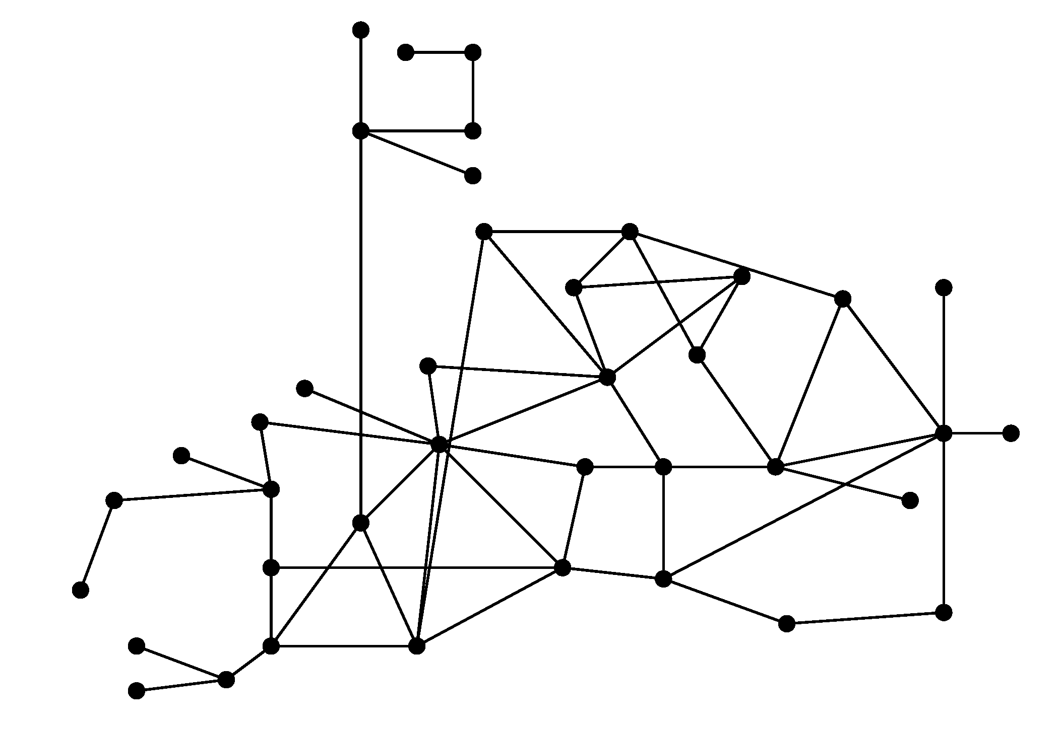
The system used as a case study is a part of the Barcelona DWN that is presented in [36]. In the considered case study, nine sources were considered, consisting of five underground and four surface sources, which currently provide an inflow of about 2 m3/s. This part is composed of 17 tanks and 61 actuators (valves and pumps), 12 nodes, and 25 demands. Figure 2 presents the considered network showing the components and the relationships between them.
The approach proposed in this paper has been applied to the using the control-oriented model of DWN presented in Figure 2 presented in Section 2. This model can also be represented by means of a graph G ( ν , ε ) , where n x storage tanks, n s sources, n d demands, and n q intersection nodes are represented by v ν vertices that are connected by a ε links (pipes) (see Figure 3). The graph that shows in figure of the water network was obtained from the state-space representation of the system. This procedure is defined with more detail in [37]. According to the DWN reliability study, demands, sources, pipelines, and tanks are considered completely reliable whereas active elements such as valves and pumps are recognized not completely reliable [38]. The forecast of each demand d ¯ m ( k ) ) is known as well the distribution of the forecasting error d ˜ m (see Figure 4).
Using the reliability analysis, the states that are structurally controllable can be determined since the path computation analysis gives all possible paths from a source to a consumer node. Furthermore, an approximate operational cost (related to the electricity cost of pump) and a maximal water flow (according to the physical constraints of the actuators) can be obtained for each path. From the definition of minimal path P s in Section 4.2, the minimal path sets are determined for Barcelona DWN. A minimal path set is composed by those components which allow a flow path between sources and demands, such as pipes, tanks, and pumps.
Table 1 and Table 2 present important number of critical actuators within the network, according to the topology and the way of network elements are linked, as most actuators (pumps or valves) have the unique connection between tanks and demands. Subsequently, if an actuator fails, then the corresponding demand will not be satisfied. Note that the information presented in Table 1 and Table 2 is particularly significant for AGBAR because it recognizes the critical elements in the network for monitoring/improvement policies to be performed in the event of element damage [39]. Considering the DWN (Figure 2), Table 1 and Table 2, and the study of the success minimal path of the water network, 607 minimal path sets are specified inside the system. Some simplification of success minimal paths from the water network is presented in Table 3.
The reliability of each minimal path set depends on the reliability of its components; tanks and pipes are supposed perfectly reliable. Although, sources are involved in the minimal path sets only for illustrative purposes of the procedure. The objective of the MPC as has been explained before is to minimize the multi-objective cost function (54). The prediction horizon is 24 h because the demand and also the electrical tariff have periodicity of 1 day. The analysis is carried for a time period of 11 day (264 h) with sampling time of 1 h. The weights of the cost function (54a) are W e = 100 , W s = 1 , W Δ u = 1 , and W R g = 10 . The weighting matrices are founded by iterative tuning until the desired performance is achieved. The tuning of these parameters is arranged based on that the objective with the highest preference is the economic cost, which must be minimized maintaining proper levels of safety volumes and control action smoothness and the same time should maximize the system reliability. The simulation results based on real data are obtained using the Gurobi 6 . 2 optimization package and Matlab R2015b (64 bits), running in a PC Intel(R) Core(TM)i7-5500 CPU at 2.4 GHz with 12 GB of RAM.

6.2. Results and Discussion

To analyze and assess the benefits of the proposed economic readability-aware MPC-LPV approach, a comparison with respect to baseline control strategies that were earlier proposed for the same case study is considered. In particular, the considered methods are as follows.
  • Reliability-Aware Chance-constrained Economic MPC-LPV (RACCEMPC-LPV): This is the approach proposed in this paper that is based on solving the optimization problem (54). This approach allows the consideration of nonstationary stochastic demand uncertainty and stochastic whole reliability of the system. Therefore, the base stock constraint, the hard bounds of the states and the terminal constraint of the system reliability are formulated in the framework of chance constraints.
  • Economic MPC-LPV (EMPC-LPV): This approach is based the optimization problem (45) without including the reliability objective. Moreover, it is not considering the stochastic demand uncertainty, chance constraints, and terminal constraint of the system reliability of the network.
  • Chance-constrained Economic MPC-LPV (CCEMPC-LPV): This approach is included robustness only for demand uncertainty by replacing the state deterministic constraints with chance-constraints. Moreover, the CCEMPC-LPV controller does not include neither the reliability objective nor the terminal constraint of the system reliability of the network.
  • Reliability-aware economic MPC-LPV (RAEMPC-LPV): This approach relies on solving problem (45a). In this approach, an additional goal is included to the controller in order to extend the components and system reliability. However, the stochastic demand uncertainty and chance constraints associated to the system reliability are not considered.
Table 4 exhibits the numeric assessment of the above-mentioned controllers through different key performance indicators (KPIs), which are detailed below,
K P I e : = 1 n s + 1 k = 0 n s α ( k ) u k Δ t , ( 55 a ) K P I Δ u : = 1 n s + 1 i = 1 n u k = 0 n s ( Δ u ( i , k ) ) 2 , ( 55 b ) K P I s : = i = 1 n x k = 0 n s max { 0 , x s ( i , k ) - x ( i , k ) } , ( 55 c ) K P I R : = x R g ( k ) , ( 55 d ) K P I t : = t o p t ( k ) , ( 55 e )
where K P I e denotes the average economic performance of the water network, K P I Δ u evaluates the smoothness of the control actions, K P I s comprises the quantity of water utilized from safety stocks, K P I R denotes the value of the whole system reliability of the DWN, and K P I t defines the difficulty to solve the optimization tasks associated with each approach accounting t o p t ( k ) as the average time that gets to solve the corresponding FHOP. In K P I e , K P I Δ u , K P I s , and K P I t lower values signify better performance results. However, a higher K P I R value shows better performance in system reliability of the DWN. Furthermore, Table 5 presents the details of the production and operational costs associated with each approach, which are one of the most important objectives for the DWN managers.
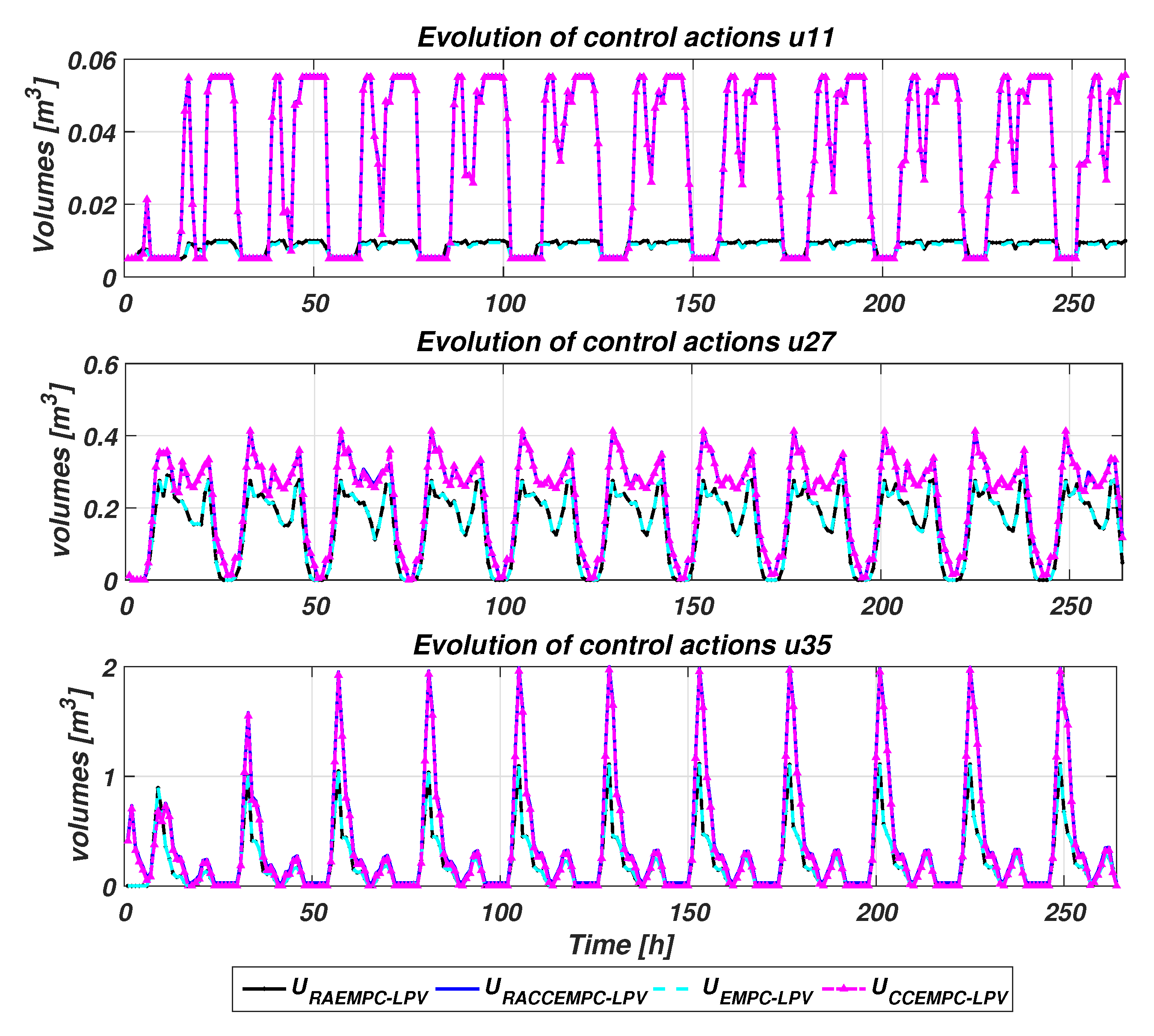
Figure 5 and Figure 6 show, respectively, the evolution of the flow actuator commands and the tank volumes for comparison of different considered MPC approaches for the Barcelona DWN. Figure 5 shows that pumps always try to operate at the minimum cost, i.e., when the electrical tariff is cheaper. Figure 6 shows the proper replenishment planning for the tanks that the predictive controller dictates according to the cyclic behavior of demands. Note that the net demand of each tank is properly satisfied along the simulation horizon.
To manage the stochastic demand uncertainty, CCEMPC-LPV and RACCEMPC-LPV controllers incorporated the robustness for demand uncertainty by replacing the state deterministic constraints with chance constraints. Generally, chance constraints create an optimal back-off from real constraints as a risk-averse mechanism to face the nonstationary uncertainty included in the prediction of states. This is reflected in Figure 5, where the behavior in the presented actuators commands in chance constraints approaches (CCEMPC-LPV and RACCEMPC-LPV) are almost the same and larger than in the case of EMPC-LPV and RAEMPC-LPV, that also present a similar behavior. Similarly, this behavior appeared in the volume evolution of the selected storage tanks that are presented in Figure 6. These results are logical since to cope with the uncertainty considered by the chance constraint-based methods additional water is stored in the tanks and this requires more flow to be injected.
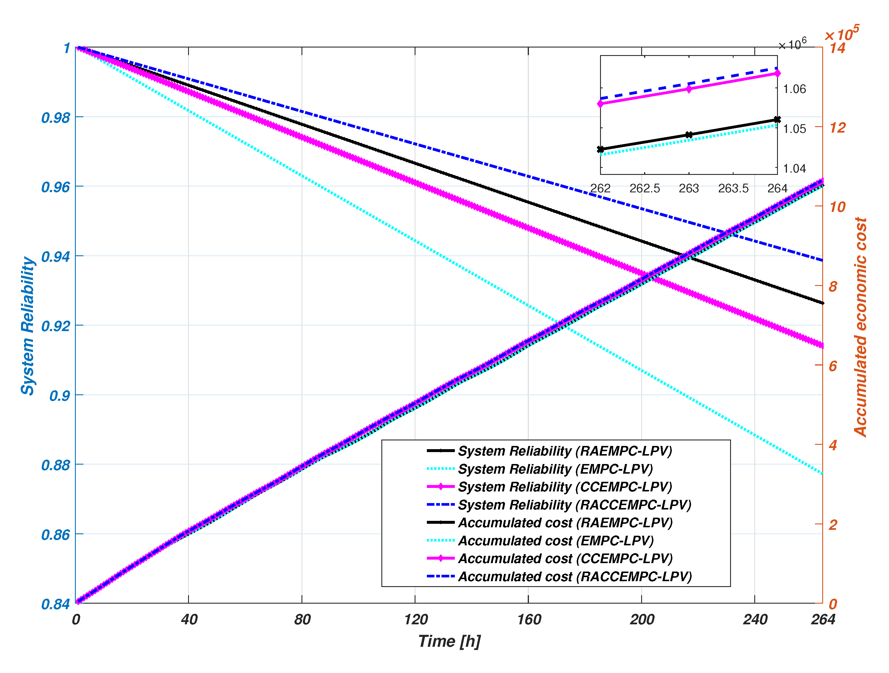
Table 5 presents the details of water production and electricity cost of each approach. The RACCEMPC-LPV approach has similar costs to those of the baseline CCEMPC-LPV approach, but with the profit of a better handling of constraints and considering the system reliability into control low of the controller. Generally, the proposed RACCEMPC-LPV approach leads to a higher total closed-loop operational cost if considering only the water and electric costs as signs for economic performance. This is the price to pay for increasing the reliability of the system.
On the other hand, Figure 7 shows the comparison of the system reliability predictions and accumulated economic cost of the DWN that obtained from the different MPC approaches. According to this figure and reviewing the results in Table 4 and Table 5, it can be observed that the robustness enhancements of the RACCEMPC-LPV approach are larger than the other controllers in terms of reliability. The EMPC-LPV controller has lower values in the economic index K P I e but, the guarantee of reliability, robustness and feasibility problems are not considered. The main disadvantage of this controller is that control actions are computed based on economic criteria. In this case, the controller overexploits actuators that have lower operational costs, quickening their damage and hazarding the service reliability. The RAEMPC-LPV strategy reached the lowest K P I e after the EMPC-LPV controller by including the reliability objective in the control low. However, the stochastic demand uncertainty and stochastic uncertainty of the system reliability are not considered.

7. Conclusions

In this paper, an economic reliability-aware LPV-MPC strategy based on chance constraints for water transport network has been proposed to deal with the management of flow-based networks, considering both demand uncertainty and system reliability in a probabilistic way. The considered control-oriented model of the water transport network is based on a flow modeling approach. By considering chance constraints programming to compute an optimal replenishment policy based on a desired risk acceptability level, the system reliability is introduced as state variables inside the control model, which includes nonlinear term and it is changed in a linear-like form through the LPV structure. Therefore, the LPV model includes both the reliability and DWN models including scheduling parameters are updated with the state vector value at that time. Moreover, nonstationary flow demands and system reliability are satisfied by considering chance-constraint programming. The results obtained show that the system reliability of the DWN network is maximized with the proposed controller while the cost is slightly increased. The level of resultant back-off volume is variable and depend of the forecast demand uncertainty and system reliability at each prediction step based on probabilistic distributions employed to their modeling. As, in practice, disturbances are unbounded, the strategy proposed in this paper is based on a service-level guarantee and a probabilistic feasibility.
Future research will concentrate on the study of predicting the system reliability of water distribution networks by considering the pressure model.

Author Contributions

All the authors have equally contributed. All authors have read and agreed to the published version of the manuscript.

Funding

This work has been partially funded by the Spanish State Research Agency (AEI) and the European Regional Development Fund (ERFD) through the projects SCAV (ref. MINECO DPI2017-88403-R) and also by EU INTERREG POCTEFA (2014-2020) EFA 153/16 SMART.

Conflicts of Interest

The authors declare no conflict of interest.

References

  1. Ocampo-Martinez, C.; Puig, V.; Cembrano, G.; Quevedo, J. Application of predictive control strategies to the management of complex networks in the urban water cycle [applications of control]. IEEE Control Syst. 2013, 33, 15–41. [Google Scholar]
  2. Karimi Pour, F.; Puig, V.; Ocampo-Martinez, C. Health-aware Model Predictive Control of Pasteurization Plant. J. Phys. 2017, 783, 12030. [Google Scholar]
  3. Maciejowski, J.M. Predictive Control: With Constraints; Pearson Education: London, UK, 2002. [Google Scholar]
  4. Cembrano, G.; Quevedo, J.; Puig, V.; Pérez, R.; Figueras, J.; Verdejo, J.; Escaler, I.; Ramón, G.; Barnet, G.; Rodríguez, P.; et al. PLIO: A generic tool for real-time operational predictive optimal control of water networks. Water Sci. Technol. 2011, 64, 448–459. [Google Scholar] [CrossRef] [PubMed]
  5. Ocampo-Martinez, C.; Ingimundarson, A.; Puig, V.; Quevedo, J. Objective prioritization using lexicographic minimizers for MPC of sewer networks. IEEE Trans. Control Syst. Technol. 2008, 16, 113–121. [Google Scholar] [CrossRef]
  6. Pascual, J.; Romera, J.; Puig, V.; Cembrano, G.; Creus, R.; Minoves, M. Operational predictive optimal control of Barcelona water transport network. Control Eng. Pract. 2013, 21, 1020–1034. [Google Scholar] [CrossRef] [Green Version]
  7. Puig, V.; Ocampo-Martinez, C.; De Oca, S.M. Hierarchical temporal multi-layer decentralised MPC strategy for drinking water networks: Application to the barcelona case study. In Proceedings of the 2012 20th Mediterranean Conference on Control & Automation (MED), Barcelona, Spain, 3–6 July 2012; pp. 740–745. [Google Scholar]
  8. Rawlings, J.B.; Mayne, D.Q. Model Predictive Control: Theory and Design; Nob Hill Pub.: Santa Barbara, CA, USA, 2009. [Google Scholar]
  9. Karimi Pour, F.; Puig, V.; Ocampo-Martinez, C. Economic Predictive Control of a Pasteurization Plant using a Linear Parameter Varying Model. In Computer Aided Chemical Engineering; Elsevier: Amsterdam, The Netherlands, 2017; Volume 40, pp. 1573–1578. [Google Scholar]
  10. Gertsbakh, I. Theory of Reliability with Applications to Preventive Maintenance; Springer: Berlin/Heidelberg, Germany, 2000. [Google Scholar]
  11. Gokdere, L.; Chiu, S.L.; Keller, K.J.; Vian, J. Lifetime control of electromechanical actuators. In Proceedings of the 2005 IEEE Aerospace Conference, Big Sky, MT, USA, 5–12 March 2005; pp. 3523–3531. [Google Scholar]
  12. Pereira, E.B.; Galvão, R.K.H.; Yoneyama, T. Model predictive control using prognosis and health monitoring of actuators. In Proceedings of the 2010 IEEE International Symposium on Industrial Electronics (ISIE), Bari, Italy, 4–7 July 2010; pp. 237–243. [Google Scholar]
  13. Karimi Pour, F.; Puig, V.; Ocampo-Martinez, C. Multi-layer health-aware economic predictive control of a pasteurization pilot plant. Int. J. Appl. Math. Comput. Sci. 2018, 28, 97–110. [Google Scholar] [CrossRef] [Green Version]
  14. Gallestey, E.; Stothert, A.; Antoine, M.; Morton, S. Model predictive control and the optimization of power plant load while considering lifetime consumption. IEEE Trans. Power Syst. 2002, 17, 186–191. [Google Scholar] [CrossRef]
  15. Khelassi, A.; Theilliol, D.; Weber, P.; Sauter, D. A novel active fault tolerant control design with respect to actuators reliability. In Proceedings of the 2011 50th IEEE Conference on Decision and Control and European Control Conference (CDC-ECC), Orlando, FL, USA, 12–15 December 2011; pp. 2269–2274. [Google Scholar]
  16. Salazar, J.C.; Sarrate, R.; Nejjari, F.; Weber, P.; Theilliol, D. Reliability computation within an MPC health-aware framework. IFAC-PapersOnLine 2017, 50, 12230–12235. [Google Scholar] [CrossRef]
  17. Salazar, J.C.; Weber, P.; Sarrate, R.; Theilliol, D.; Nejjari, F. MPC design based on a DBN reliability model: Application to drinking water networks. IFAC-PapersOnLine 2015, 48, 688–693. [Google Scholar] [CrossRef]
  18. Karimi Pour, F.; Puig, V.; Cembrano, G. Health-aware LPV-MPC based on system reliability assessment for drinking water networks. In Proceedings of the 2nd IEEE Conference on Control Technology and Applications, Copenhagen, Denmark, 21–24 August 2018. [Google Scholar]
  19. Chamseddine, A.; Theilliol, D.; Sadeghzadeh, I.; Zhang, Y.; Weber, P. Optimal reliability design for over-actuated systems based on the MIT rule: Application to an octocopter helicopter testbed. Reliab. Eng. Syst. Saf. 2014, 132, 196–206. [Google Scholar] [CrossRef]
  20. Grosso, J.M.; Ocampo-Martínez, C.; Puig, V. A service reliability model predictive control with dynamic safety stocks and actuators health monitoring for drinking water networks. In Proceedings of the 2012 IEEE 51st Annual Conference on Decision and Control (CDC), Maui, HI, USA, 10–13 December 2012; pp. 4568–4573. [Google Scholar]
  21. Karimi Pour, F.; Puig Cayuela, V.; Ocampo-Martínez, C. Comparative assessment of LPV-based predictive control strategies for a pasteurization plant. In Proceedings of the 4th—2017 International Conference on Control, Decision and Information Technologies, Barcelona, Spain, 5–7 April 2017; pp. 1–6. [Google Scholar]
  22. Calafiore, G.C.; Dabbene, F.; Tempo, R. Research on probabilistic methods for control system design. Automatica 2011, 47, 1279–1293. [Google Scholar] [CrossRef]
  23. Schwarm, A.T.; Nikolaou, M. Chance-constrained model predictive control. AIChE J. 1999, 45, 1743–1752. [Google Scholar] [CrossRef]
  24. Geletu, A.; Klöppel, M.; Zhang, H.; Li, P. Advances and applications of chance-constrained approaches to systems optimization under uncertainty. Int. J. Syst. Sci. 2013, 44, 1209–1232. [Google Scholar] [CrossRef]
  25. Ouarda, T.; Labadie, J. Chance-constrained optimal control for multireservoir system optimization and risk analysis. Stoch. Environ. Res. Risk Assess. 2001, 15, 185–204. [Google Scholar] [CrossRef]
  26. Mays, L. Urban Stormwater Management Tools; McGraw Hill Professional: New York, NY, USA, 2004. [Google Scholar]
  27. Brdys, M.; Ulanicki, B. Operational Control of Water Systems: Structures, Algorithms and Applications. Automatica 1996, 32, 1619–1620. [Google Scholar]
  28. Cembrano, G.; Quevedo, J.; Salamero, M.; Puig, V.; Figueras, J.; Martı, J. Optimal control of urban drainage systems. A case study. Control Eng. Pract. 2004, 12, 1–9. [Google Scholar] [CrossRef]
  29. Kall, P.; Mayer, J. Stochastic Linear Programming; Springer: Berlin/Heidelberg, Germany, 1976; Volume 7. [Google Scholar]
  30. Grosso, J.M.; Velarde, P.; Ocampo-Martinez, C.; Maestre, J.M.; Puig, V. Stochastic model predictive control approaches applied to drinking water networks. Optim. Control Appl. Methods 2017, 38, 541–558. [Google Scholar] [CrossRef] [Green Version]
  31. Nemirovski, A.; Shapiro, A. Convex approximations of chance constrained programs. SIAM J. Optim. 2006, 17, 969–996. [Google Scholar] [CrossRef]
  32. Shapiro, A.; Dentcheva, D.; Ruszczyński, A. Lectures on Stochastic Programming: Modeling and Theory; SIAM: Phhiladelphia, PA, USA, 2009. [Google Scholar]
  33. Jiang, R.; Jardine, A.K. Health state evaluation of an item: A general framework and graphical representation. Reliab. Eng. Syst. Saf. 2008, 93, 89–99. [Google Scholar] [CrossRef]
  34. Gertsbakh, I. Reliability Theory: With Applications to Preventive Maintenance; Springer: Berlin/Heidelberg, Germany, 2013. [Google Scholar]
  35. Baecher, G.B.; Christian, J.T. Reliability and Statistics in Geotechnical Engineering; John Wiley & Sons: Hoboken, NJ, USA, 2005. [Google Scholar]
  36. Ocampo-Martínez, C.; Puig, V.; Cembrano, G.; Creus, R.; Minoves, M. Improving water management efficiency by using optimization-based control strategies: The Barcelona case study. Water Sci. Technol. Water Supply 2009, 9, 565–575. [Google Scholar] [CrossRef]
  37. Siljak, D.D. Decentralized Control of Complex Systems; Courier Corporation: Chelmsford, MA, USA, 2011. [Google Scholar]
  38. Weber, P.; Simon, C.; Theilliol, D.; Puig, V. Fault-Tolerant Control Design for over-actuated System conditioned by Reliability: A Drinking Water Network Application. IFAC Proc. Vol. 2012, 45, 558–563. [Google Scholar] [CrossRef] [Green Version]
  39. Robles, D.; Puig, V.; Ocampo-Martinez, C.; Garza-Castañón, L.E. Reliable fault-tolerant model predictive control of drinking water transport networks. Control Eng. Pract. 2016, 55, 197–211. [Google Scholar] [CrossRef] [Green Version]
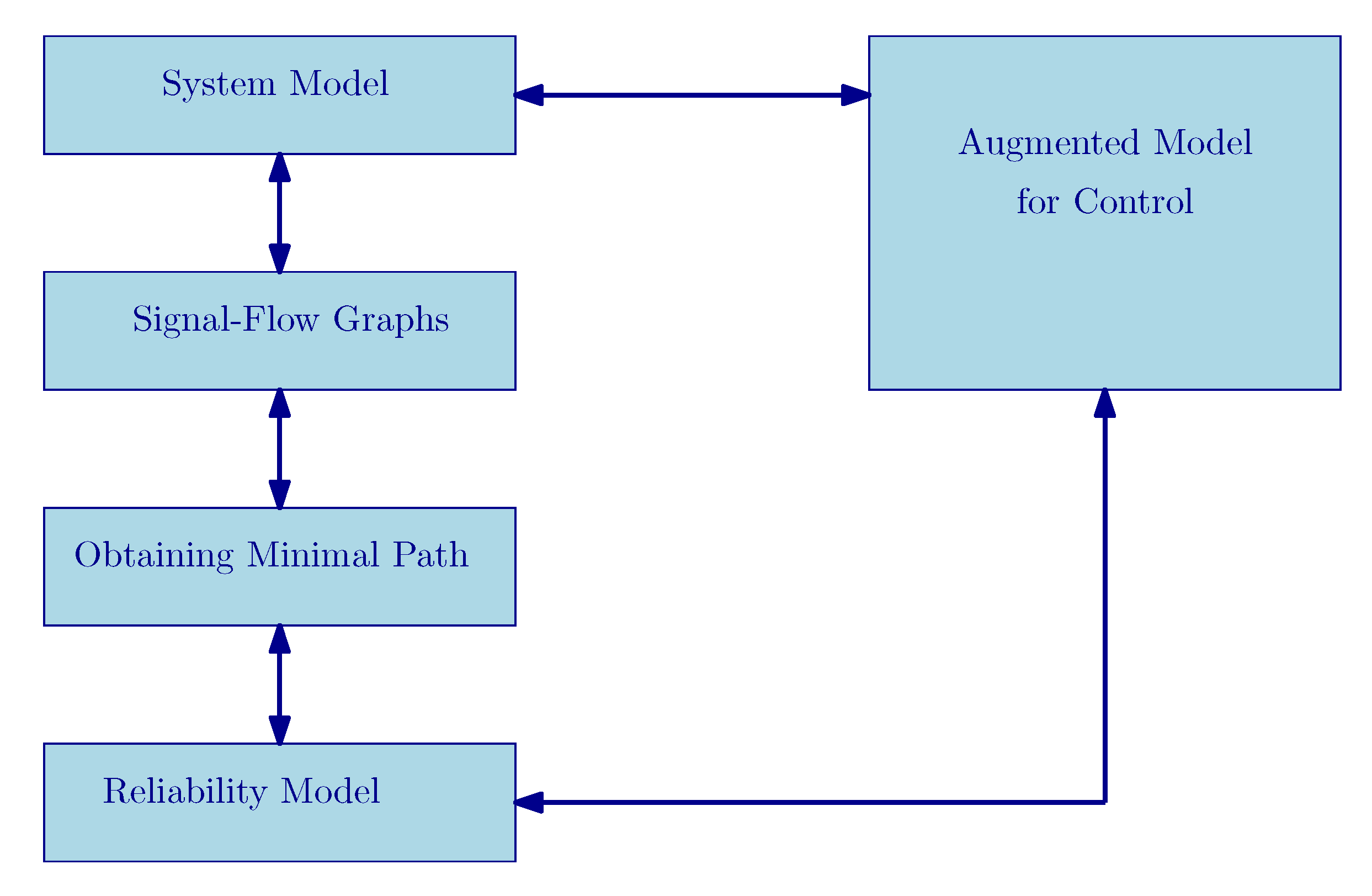
Figure 1. Structure diagram of the proposed approach.
Processes 08 00060 g001
Figure 2. Barcelona drinking water network.
Processes 08 00060 g002
Figure 3. Graph from Barcelona DWN.
Processes 08 00060 g003
Figure 4. Drinking water demand for several demands.
Processes 08 00060 g004
Figure 5. Evaluation of the control actions results.
Processes 08 00060 g005
Figure 6. Results of the evolutions of storage tanks.
Processes 08 00060 g006
Figure 7. Evaluation of system reliability and accumulated economic cost.
Processes 08 00060 g007
Table 1. Structural actuators (towards tanks).
No.NameNo.NameNo.NameNo.Name
u 1 VALVA u 16 VALVA309 u 33 CC130 u 47 VPSJ
u 3 CPIV u 17 bPousE u 34 CC70 u 48 CMO
u 4 bMS u 19 CGIV u 35 VB u 49 VMC
u 5 CPII u 20 CPLANTA50 u 36 CF176 u 50 VALVA60
u 6 VALVA47 u 21 PLANTA10 u 37 VCO u 51 VALVA56
u 7 bCast u 23 CRE u 38 CCO u 52 VALVA57
u 8 VCR u 24 CC100 u 39 VS u 53 CRO
u 9 bPouCast u 25 VALVA64 u 40 V u 54 VBMC
u 10 CCA u 26 VALVA50 u 41 VCT u 55 bPousB
u 11 CB u 27 CC50 u 42 CA u 56 VALVA53
u 12 VALVA308 u 28 VF u 43 VP u 57 VALVA54
u 13 VALVA48 u 29 CF200 u 44 VBSLL u 58 VALVA61
u 14 VCA u 30 VE u 45 CPR u 59 VALVA55
u 15 CPLANTA70 u 32 VZF u 46 VCOA u 60 VCON
Table 2. Structural actuators (towards demands).
No.NameNo.NameNo.NameNo.Name
u 2 VALVA45 u 18 VSJD-29 u 22 CE u 31 VRM
u 61 VALVA312
Table 3. Success minimal paths of the Barcelona DWN.
PathComponent Set
P 1 a M S , b M S , c 125 P A L
P 2 A p o r t A , V A L V A , V A L V A 45 , c 70 P A L
P 3 A p o r t A , V A L V A , V A L V A 47 , C P I V , c 125 P A L
P 4 A p o r t A , V A L V A , C P I I , c 110 P A P
P 5 A C a s t , b C a s t , c 115 C A S T
                  ⋮
P 607 A p o r t T , V A L V A 312 , c 135 S C G
Table 4. Comparison of control performance.
Controller KPI e KPI Δ u KPI s KPI Rg KPI t Simulation Time
EMPC-LPV3779.810.527128951.720.87721.5628412.599
CCEMPC-LPV4029.090.491028955.690.91861.9051502.952
RAEMPC-LPV3980.070.531728952.620.92631.78348470.841
RACCEMPC-LPV4029.190.490328955.900.93861.9664519.147
Table 5. Comparison of daily average costs of the MPC approaches.
MPC Approach   Water Average CostElectric Average CostDaily Average Cost
(e.u./day)(e.u./day)(e.u./day)
EMPC-LPV44162.443053.0847215.53
CCEMPC-LPV51237.983262.4354500.42
RAEMPC-LPV44369.903121.8447491.75
RACCEMPC-LPV51438.133262.6454700.77