A Hybrid Inverse Problem Approach to Model-Based Fault Diagnosis of a Distillation Column

Abstract

Early-stage fault detection and diagnosis of distillation has been considered an essential technique in the chemical industry. In this paper, fault diagnosis of a distillation column is formulated as an inverse problem. The nonlinear least squares algorithm is used to evaluate fault parameters embedded in a nonlinear dynamic model of distillation once abnormal symptoms are detected. A partial least squares regression model is built based on fault parameter history to explicitly predict the development of fault parameters. With the stripper of Tennessee Eastman process as example, this novel approach is tested for step- and random-type faults and several factors affecting its efficiency are discussed. The application result shows that the hybrid inverse problem approach gives the correct change of fault parameter at a speed far faster than the base approach with only a nonlinear model.

1. Introduction

Distillation is a widely used energy consuming unit operation in modern petroleum and chemical industries. Its separation on raw materials, intermediate products, and crude products exerts a strong influence on the energy consumption and product quality of the industrial process involved. The fault diagnosis technique benefits from catching the deterioration symptom of critical parameters in time and predicting their deterioration trend effectively when a distillation column enters an abnormal state. To improve the reliability of control systems, the problem of fault detection and diagnosis has been paid more attention over the past two decades. A robust fault diagnostic method for multiple open-circuit faults and current sensor faults in three-phase permanent magnet synchronous motor drives has been proposed by Jlassi [1]. The proposed observer-based algorithm relies on an adaptive threshold for fault diagnosis. A composite fault tolerant control (CFTC) with disturbance observer scheme has been considered for a class of stochastic systems with faults and multiple disturbances [2]. The problem of fault diagnosis for a class of nonlinear systems has been investigated via the hybrid method of an observer-based approach and homogeneous polynomials technique [3]. As one of the quantitative model-based fault diagnosis methods for the distillation process, the parameter estimation method identifies the process parameters of physical meaning, such as the heat transfer coefficient, thermal resistance, etc., and hereby explains abnormal reasons based on the relationship between input and output signals. From the point of view of control theory, the parameter estimation method provides a closed loop structure with a good computational stability and convergence since parameters are input into the reasoning model again after estimation. Based on a nonlinear dynamic model, parameter estimation, however, becomes a nonlinear optimization problem, whose heavy computational load is a serious bottleneck limiting its application. Some improvements have therefore emerged in the last decade to simplify both the model and algorithm. For example, a hybrid fault detection and diagnosis scheme was implemented in a two-step pattern, that is, neural networks were activated to deduce the root reason for a fault state after the fault-related section of a plant was located by a Petri net [4]. A fault diagnosis technique was proposed based on multiple linear models, in which several linear perturbation models suitable for various operation regimes were identified by a Bayesian approach and then combined with a generalized likelihood ratio method to perform fault identification tasks [5]. A fault detection and diagnosis scheme, which uses one tier of a nonlinear rigorous model and another tier of a linear simplified model to monitor the distillation process and identify abnormal parameters, respectively, was developed to consider the accuracy and speed of nonlinear and linear models simultaneously [6]. A three-layer nonlinear Gaussian belief network was constructed and trained to extract useful features from noisy process data, where the absolute gradient was monitored for fault detection and a multivariate contribution plot was generated for fault diagnosis [7].

The determination of fault parameters on the basis of known input and output signals of distillation can be approached as the solution of an inverse problem [8,9,10]. The most widely used method to solve such a problem is its least squares (LSQ) formulation as the minimization of an error function between the real measurements and their calculated values, similar to the above improved parameter estimation methods. Meanwhile, meta-heuristics for LSQ optimization are popular due to their inherent advantages, like their global optimum and the few requirements for problem formulation [11,12]. However, the running speed of the LSQ-based method is slow owing to its time-consuming iterative optimization of fault parameters. During iterations, the process of solving the forward problem and then adjusting its parameters is repeated until the difference between the measured values and the calculated ones reaches a minimum. For this reason, a direct derivation of fault parameters from input and output signals instead of trial and error in forward problems is a very current topic, such as the decomposition of solution space followed by polynomial approximation [13], usage of artificial neural networks (ANN) for the automated reconstruction of an inhomogeneous object as pattern recognition [14], and inverse regression between the disturbance and characteristic distances based on single variable perturbation [15].

Based on the LSQ-based fault diagnosis work [16], a hybrid inverse problem approach that uses partial least squares (PLS) to fit and forecast trajectories of the fault parameters generated by LSQ is proposed in this paper to accelerate the model-based fault diagnosis process. PLS is a popular tool for key performance monitoring, quality control, and fault diagnosis in large-scale chemical industry [17,18]. It has been improved from relative contributions of process variables or blocks on faults [19,20], and the orthogonal decomposition of measurement space before deducing new specific statistics with non-overlapped domains [21].

This work aims to test the feasibility of an LSQ and PLS combined hybrid inverse problem approach for model-based fault diagnosis. In the following sections, the proposed hybrid inverse problem solving approach is explained and its positive action in terms of speeding up the diagnosis process is proved via a case study of a stripper simulator in the Tennessee-Eastman process (TEP) compared to the base approach with LSQ only. The effect of initial values, iteration times, calling period, etc. on the performance of the proposed method is also analyzed.

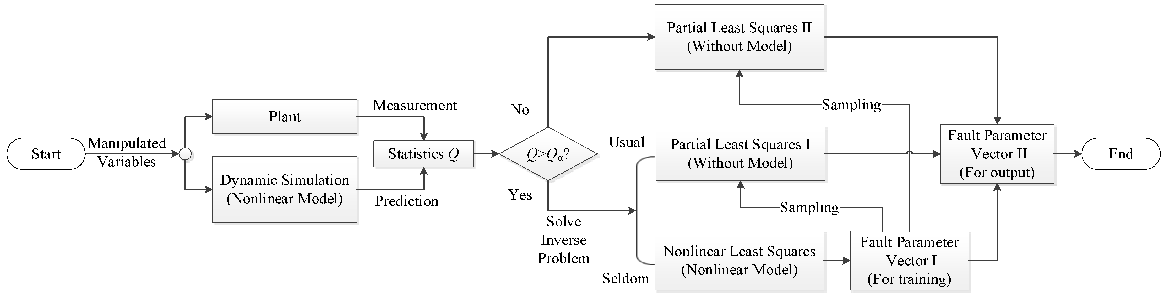
2. Hybrid Fault Diagnosis Structure

Figure 1 shows the structure of fault diagnosis formulated as a parameter-estimation inverse problem solved by the least squares optimization algorithm. The first step is fault detection, in which the system outputs estimated by dynamic simulation with a nonlinear model are compared with those measured online from a plant to check whether the present state adheres to its theoretical estimation. The difference is defined by statistic Q. When Q is greater than its threshold Q_α, the process is considered as deviating from its predefined state and the second step, fault diagnosis, is conducted. Otherwise, the fault detection step continues. Before fault diagnosis, a dynamic simulation based on the process model should be firstly performed to check its coincidence with real measurements from a plant under normal conditions. In this procedure, the model is manually calibrated to guarantee the later detected anomaly coming from a fault occurring in the plant other than an error of the model [16]. During fault diagnosis, fault parameters are obtained as a solution of an inverse problem with LSQ and PLS. PLS regression of fault parameters generated by LSQ is utilized to predict fault parameters. PLS also runs when the statistic Q lies within its threshold Q_α to give continuous fault parameter estimation. Therefore, the aforementioned hybrid inverse problem approach to parameter estimation is composed of one complex optimization part with a nonlinear model and another simple regression part with a linear model.

In Figure 1, the nonlinear model is solved once for dynamic simulation at one sampling interval to detect any fault, but is solved many times for fault diagnosis. Therefore, fault diagnosis consumes more computation time than dynamic simulation based on the same nonlinear model. The hybrid inverse problem-solving strategy replaces LSQ with PLS as much as possible since PLS calculates fault parameters directly after fitting the relationship of system outputs and fault parameters. Therefore, such a hybrid inverse problem approach can be expected to reduce the calculation load of fault diagnosis greatly.

2.1. Obtaining Fault Parameters by the LSQ Algorithm

The nonlinear fault parameters can be obtained rigorously by minimizing the deviation of measurable variables from their unsteady-state simulation values. The deviation r is defined in Equation (1) with a normalized version, Equation (2), where y_meas and y_sim represent data measured and simulated, respectively. It indicates an anomaly when its aggregated index Q exceeds the corresponding threshold Q_α, as defined in Equations (3) and (4). In this phase, fault parameters θ are solved based on an optimization formulation (LSQ) of fault parameters about the mechanism model of distillation composed of measurable variables y, manipulated variables u, disturbance ω, and state variables x, as shown in Equation (5).

$$\mathbf{r}={\mathbf{y}}_{\mathrm{meas}}-{\mathbf{y}}_{\mathrm{sim}}$$

(1)

$${\mathbf{r}}^{\ast }=\frac{\mathbf{r}-{\mathbf{r}}_{\mathrm{mean}}}{{\mathsf{\sigma }}_r}$$

(2)

$$\mathbf{Q}={\mathbf{r}}^{\ast \mathrm{T}}{\mathbf{r}}^{\ast }$$

(3)

$$Q_{\alpha }={\chi }_{\alpha }^2(m)$$

(4)

$$\begin{array}{l}\underset{{\mathsf{\theta }}_t}{\min }\mathbf{Q}\\ \mathrm{s}.\mathrm{t}.\mathbf{y}=f(\mathbf{u},\mathsf{\omega },\mathbf{x},\mathsf{\theta })\end{array}$$

(5)

As LSQ is essentially nonlinear, it is time-consuming and should not be performed frequently in practice. In a small enough range of one time point, fault parameter θ can be considered as a linear function of measurable variable y (see Equations (6) and (7)). In the present study, y and θ are scalar variables. Therefore, a revised multiple linear regression method (PLS) is used in this paper to obtain the explicit correlation between fault parameters and measurable variables.

$$\mathbf{y}=f\left(\mathsf{\theta }\right)\approx f\left({\mathsf{\theta }}_0\right)+f^{\prime }\left({\mathsf{\theta }}_0\right)\left(\mathsf{\theta }-{\mathsf{\theta }}_0\right)$$

(6)

$$\mathsf{\theta }=\frac{1}{f^{\prime }\left({\mathsf{\theta }}_0\right)}\left[\mathbf{y}-f\left({\mathsf{\theta }}_0\right)\right]+{\mathsf{\theta }}_0$$

(7)

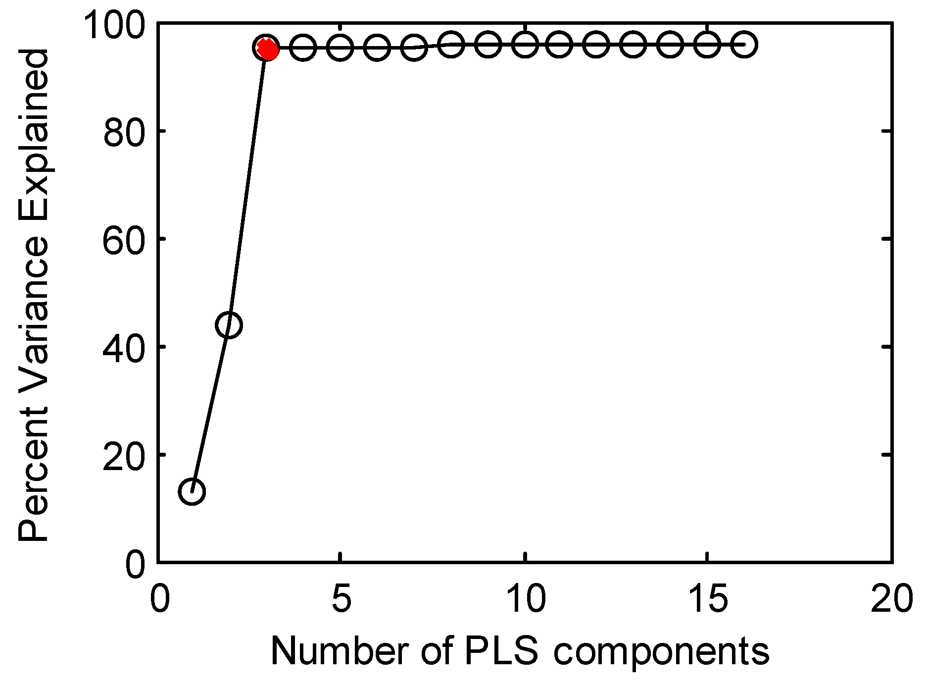
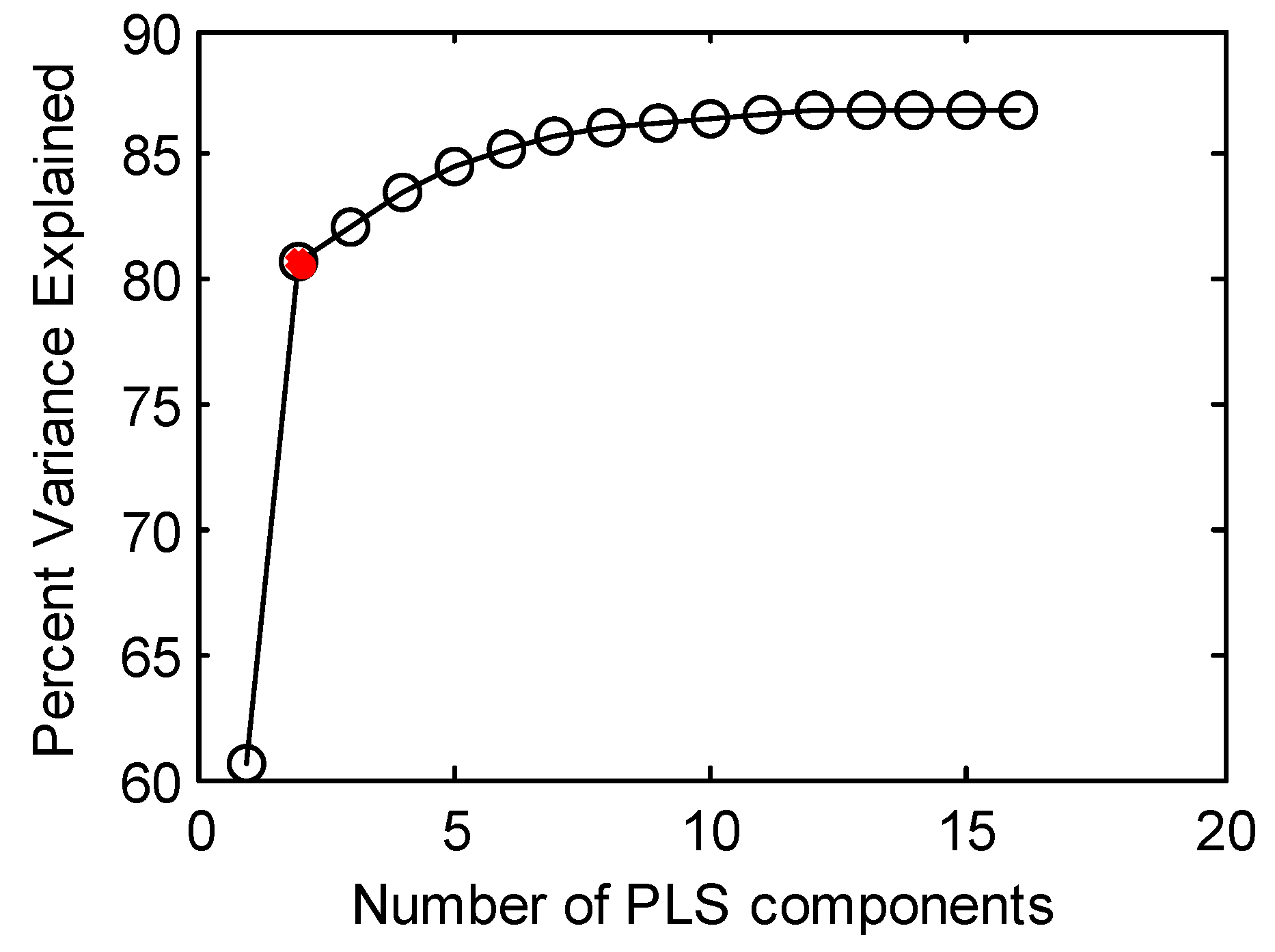
2.2. Obtaining Fault Parameters by the PLS Algorithm

Most PLS methods are applied to regression modeling, replacing the general multivariate regression and principal component regression to a large extent. Comparatively, PLS can not only exclude the correlation of original variables, but also filter the noise of both independent variables and dependent variables. Its prediction ability is stronger and more stable because it uses fewer characteristic variables to describe the regression model.

Firstly, the data X = [y u]^T∊R^l×n and Y = θ∊R^l×c are normalized and decomposed, respectively, where T, P, and E denote the score, load, and residual matrix of X, respectively; U, Q, and F denote the score, load, and residual matrix of Y, respectively; and a and n denote the number of PLS components and variables, respectively. The external relations are obtained as Equations (8) and (9).

$$\mathbf{X}={\mathbf{T}}_a{\mathbf{P}}_a^{\mathrm{T}}+\mathbf{E},a<n$$

(8)

$$\mathbf{Y}={\mathbf{U}}_a{\mathbf{Q}}_a^{\mathrm{T}}+\mathbf{F},a<n$$

(9)

Then, their internal relationship is determined as Equation (10).

$${\mathbf{U}}_a={\mathbf{T}}_a\mathbf{B},$$

(10)

where B is the internal regression matrix.

The PLS model is finally obtained as Equation (11).

$$\mathbf{Y}={\mathbf{T}}_a\mathbf{B}{\mathbf{Q}}_a^{\mathrm{T}}+\mathbf{F}$$

(11)

When the independent variable X is known, PLS can be used to predict the dependent variable Y. The calculation procedure is given in Equations (12) and (13).

$${\widehat{\mathbf{t}}}_h={\mathbf{E}}_{h-1}{\mathbf{w}}_h$$

(12)

$${\mathbf{E}}_h={\mathbf{E}}_{h-1}-{\widehat{\mathbf{t}}}_h{\mathbf{p}}_h^{\mathrm{T}},$$

(13)

where t and p represent the element vector in the score and load matrix, respectively; w represents the weight vector; h denotes the component index; and E₀ = X.

Therefore, dependent variables can be predicted using Equation (14).

$$\mathbf{Y}={\displaystyle \sum _{h=1}^a{\mathbf{v}}_h{\widehat{\mathbf{t}}}_h{\mathbf{q}}_h^{\mathrm{T}}}$$

(14)

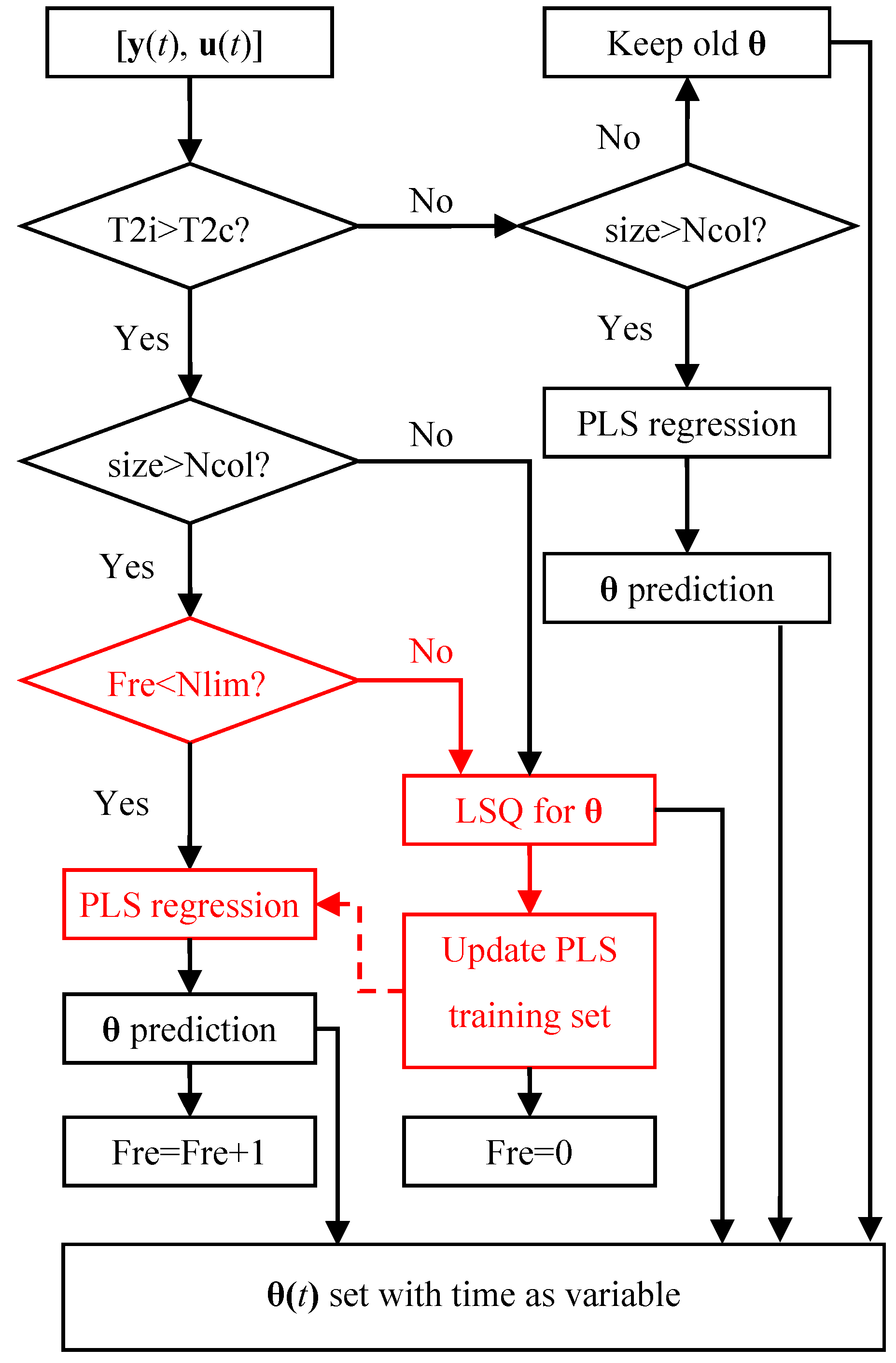
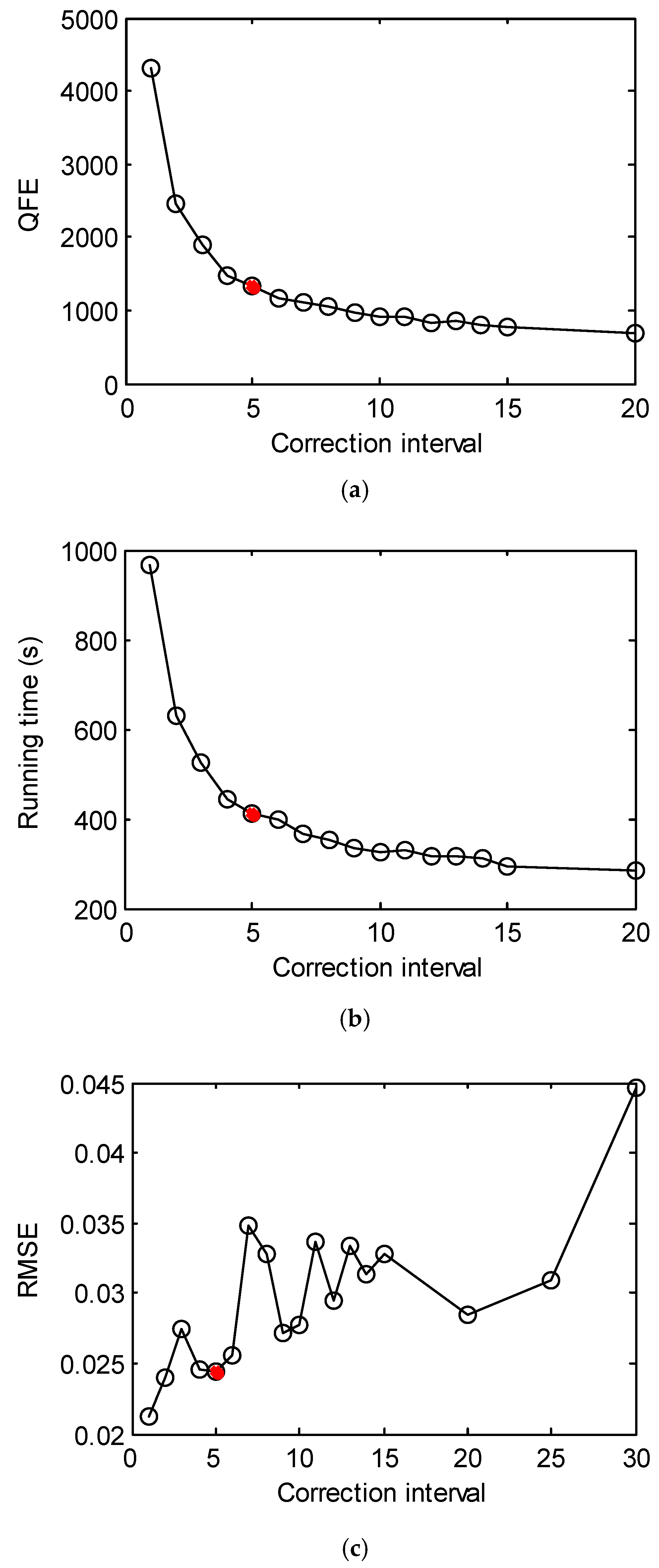
2.3. Correcting PLS by LSQ

Because PLS extracts linear features of fault parameters, it should be corrected continuously by LSQ. The correction framework is shown in Figure 2, where the red color loop represents the correction process. The rigorous iterative LSQ is performed once to supply one accurate value of fault parameters for the PLS training set when an anomaly is detected, not enough sampling points are collected, and correction is needed. The main contribution of this work lies in the frequent usage of fast PLS prediction of fault parameters instead of slow LSQ in the fault diagnosis algorithm. However, compared to LSQ, PLS’ accuracy is limited because of its linear regression essence, so it should be corrected periodically by rigorous LSQ results. Sufficient LSQ results are needed to form the training set of the PLS model before PLS correction. Therefore, if not enough sampling points of fault parameters are given by LSQ for PLS training, LSQ should be activated correspondingly to supply one sampling point of fault parameters into the PLS training set to meet the periodical correction requirements of PLS. In this case, the boundary value θ₀ in Equation (7) is kept stable and accurate, and the prediction accuracy of PLS is guaranteed as a consequence.

3. Case Study

The stripper of the TEP simulator [22] is used as an example to test the feasibility of the proposed hybrid inverse problem approach to fault diagnosis. The fault set related to this stripper includes two types, that is, a step and a random type. This work chooses fault 7 and 8 as typical examples for these two types. The advantages and disadvantages of this approach are illustrated in comparison with the base approach with LSQ only.

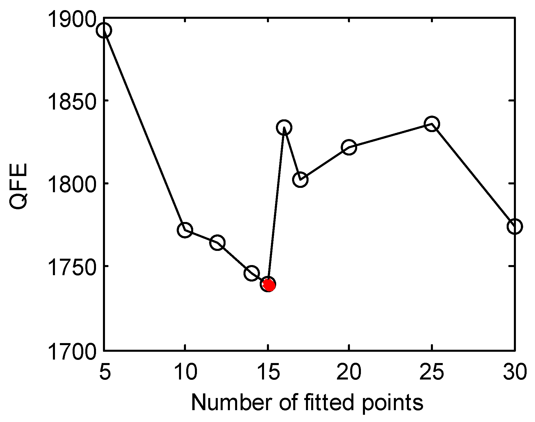
3.1. Solving the LSQ Inverse Problem with Different Initial Values

LSQ is greatly affected by the initial values of iterated variables, so the first step is to discuss different setting methods for initial values of the LSQ algorithm. The following test is firstly based on the fault diagnosis process under fault 7. Fault 7 occurs at 8 h when the header pressure loss of the stripping stream entering the stripper bottom decreases abruptly. The fault diagnosis result using LSQ only is given in Figure 3 and Figure 4, which has been published in our early work [16], henceforth referred to as the base case for comparison. In this base case, the overall running time and quantity of function evaluations (QFE) are 539 seconds and 1826, respectively. In the fault diagnosis algorithm, the boundary state at t = 0 is considered a normal state, this is, without anomaly. Therefore, the pressure loss coefficient is set as 1 uniformly in Figure 3. When t > 0, the fault diagnosis algorithm is activated to obtain the pressure loss coefficient in a timely manner based on the measurements of a plant.

(1) Set the initial value with the previous time point

The simplest value-setting method for the initial value is to directly use one from a previous time point. If there are only small changes in the fault parameter between two consecutive time points, the initial value given can thus be accepted. This is also the initial value-setting method adopted by the base case.

(2) Set the initial value with the linear fitting method

Figure 5 shows the diagnosis result with initial values given by the linear fitting method. It indicates that QFE decreases greatly and becomes stochastically stable before the fitted point number equals 30. After that, a rising function evaluation number curve is seen because of the growing time lag of the fitted line. For this reason, 5 or 8 is chosen as the candidate for the optimal fitting point number. Because more fitting points will definitely lead to a heavier computational load for the fitting operation, 5 is finally chosen as the optimal fitting point number. Despite this, QFE is only cut down by 2%, contributing little to the computational efficiency of the diagnosis algorithm.

(3) Set the initial value with the parabolic fitting method

Following the linear fitting method presented above, the parabolic fitting method, the simplest nonlinear fitting method, is utilized here to predict the initial values. Figure 6 shows the diagnosis result with this method, revealing a larger QFE than the base case. This reflects the essentially linear change of the fault parameter between neighboring time points. Therefore, the nonlinear fitting method does not achieve the satisfactory goal of reducing QFE.

(4) Set the initial value with the grey model

Different from the above regression methods, grey system theory uses partial description information of a system to generate a grey sequence revealing the potential rule of data with the goal of system whitening [23]. It has advantages such as a small amount of data, fast operation, easy iteration, and high accuracy [24]. Figure 7 gives the diagnosis result with the grey model-predicted initial values. It shows that QFE decreases by 4.7% at most when adopting 15 as the number of sampling points. So far, the highest reduction ratio of function evaluations to the base case has been obtained by the grey model, which is, therefore, the best method for estimating initial values. At the same time, the limited improvement given by the grey model shows the need for further improvement of the diagnosis algorithm based on other factors.

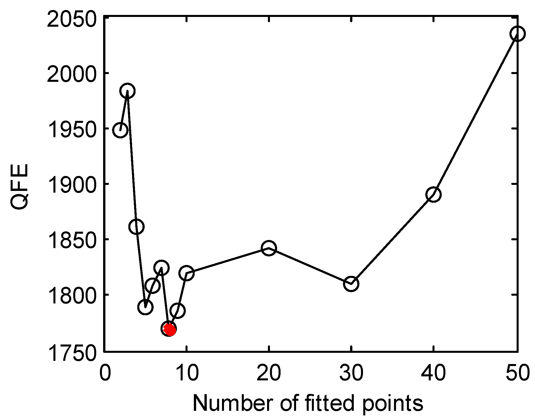
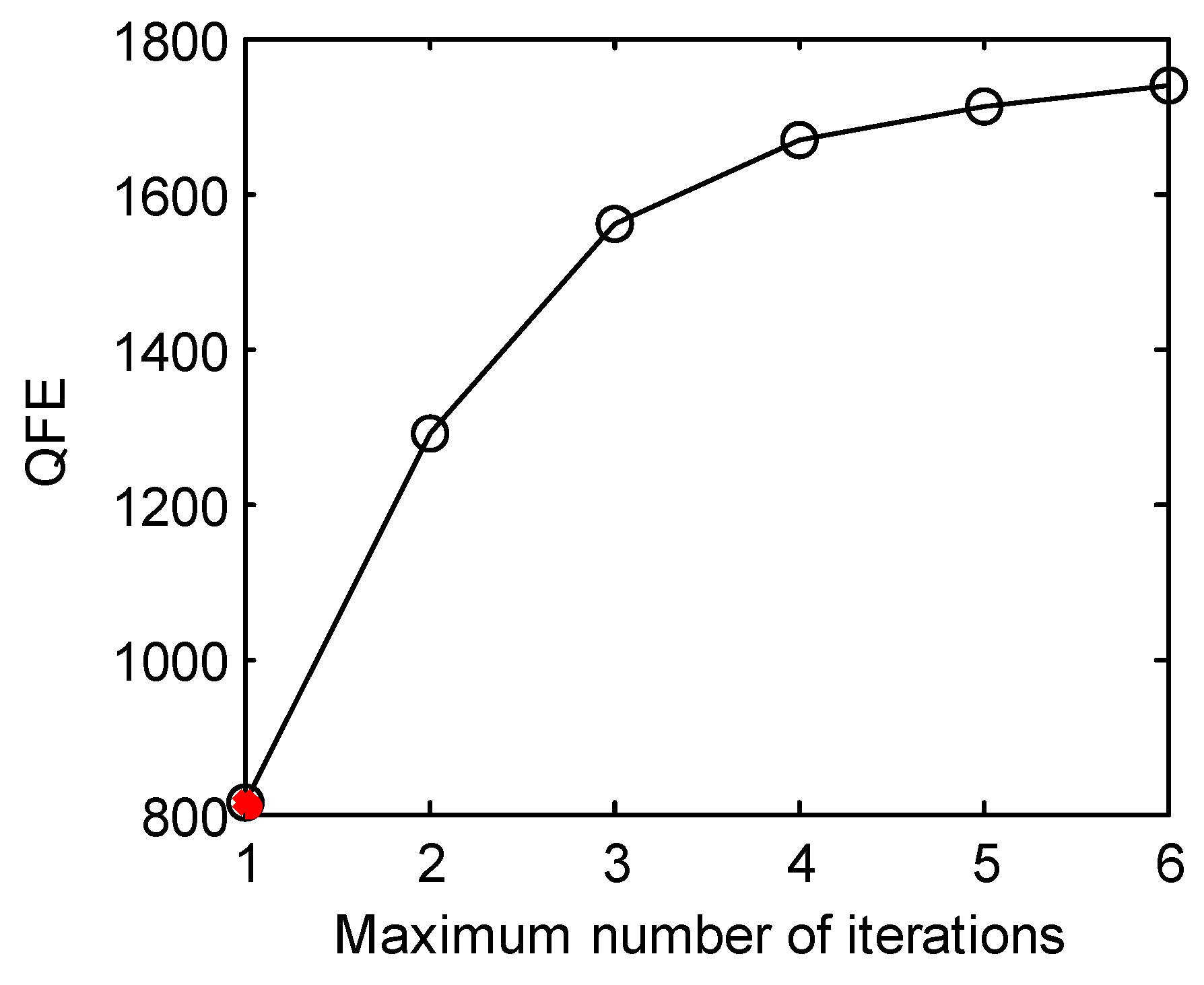
3.2. Solving the LSQ Inverse Problem with Different Numbers of Iterations

As one popular optimization algorithm, LSQ requires a large number of iterations to obtain accurate fault parameters at each sampling time, so its high computational cost is its main disadvantage. In fact, the aim of fault diagnosis is to find the abnormal trend of fault parameters in a timely manner during a given time interval. In this process, completely converged calculation at each time point is not necessary. Based on the idea of tracking approximation, the proposal of the present paper distributes the inner iterative computation into an outer integration progress to decrease the maximum number of iterations at each sampling point. Figure 8 shows the diagnosis result with different maximum numbers of iterations. It presents a great decrease of QFE when reducing the maximum number of iterations. In particular, when the iteration number equals 1, QFE decreases by 55% compared to the base case, being far greater than the value obtained by the grey model.

The fault diagnosis result obtained by this strategy is shown in Figure 9, in contrast with that obtained by the base case. The exact coherence of fault parameters between these two cases evidences no loss of accuracy with this fast algorithm. Meanwhile, minor parameter fluctuation is observed due to the insufficient iterative computation of this algorithm.

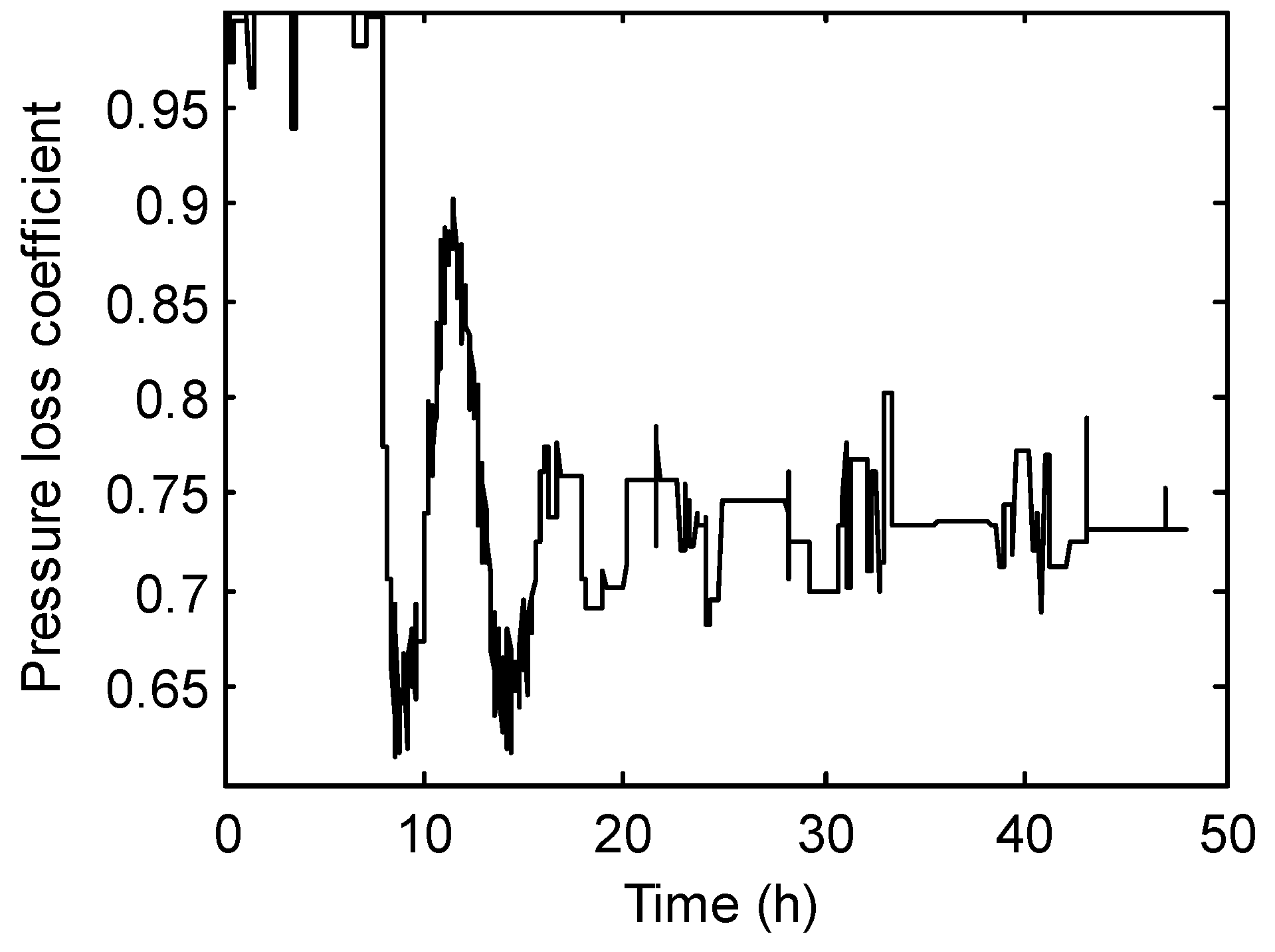
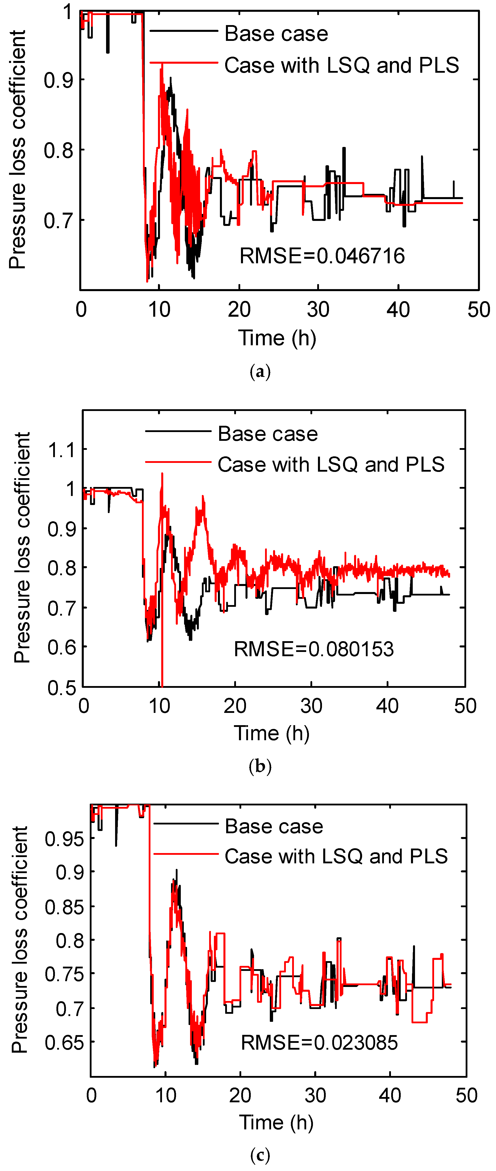
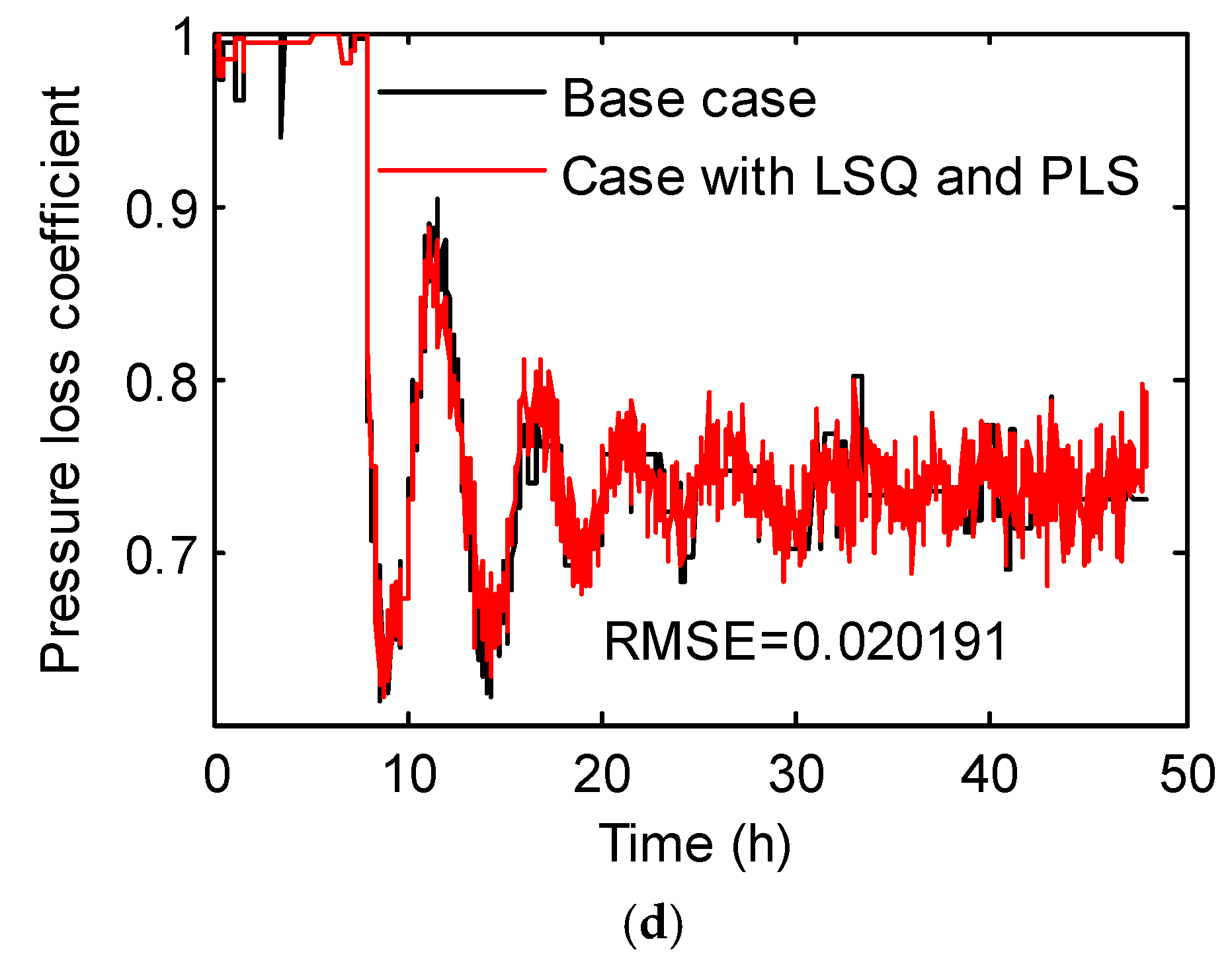
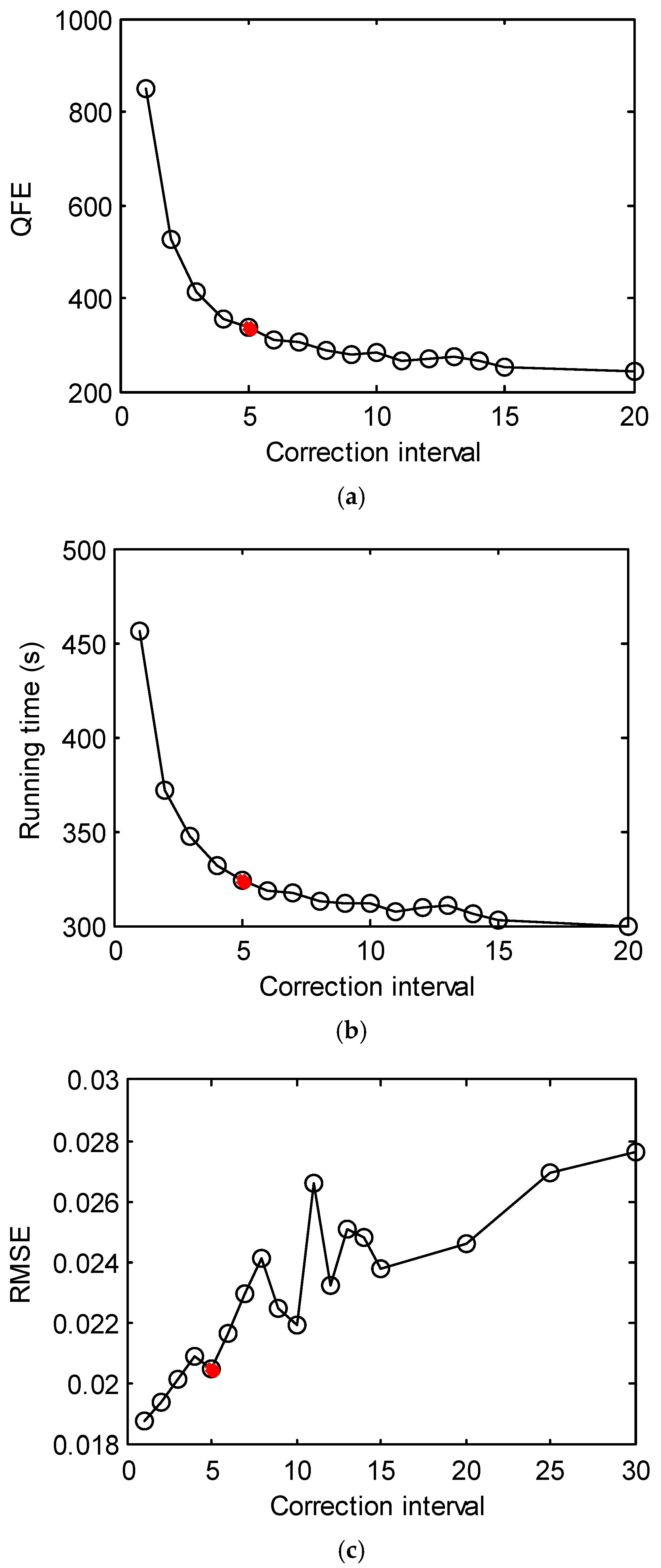
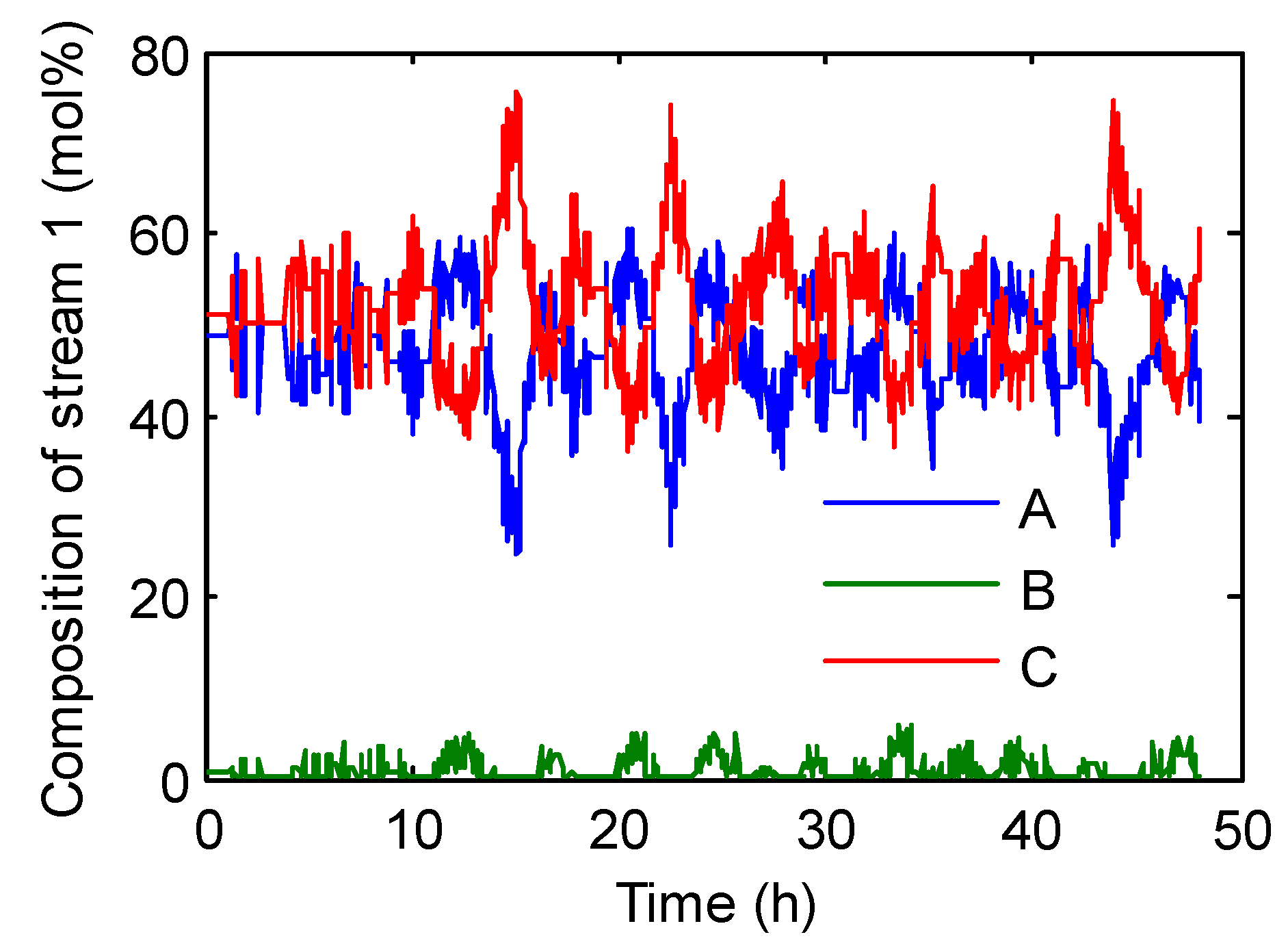
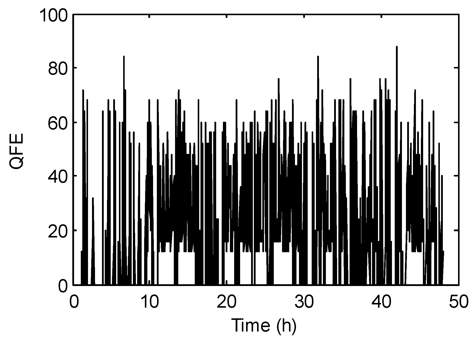
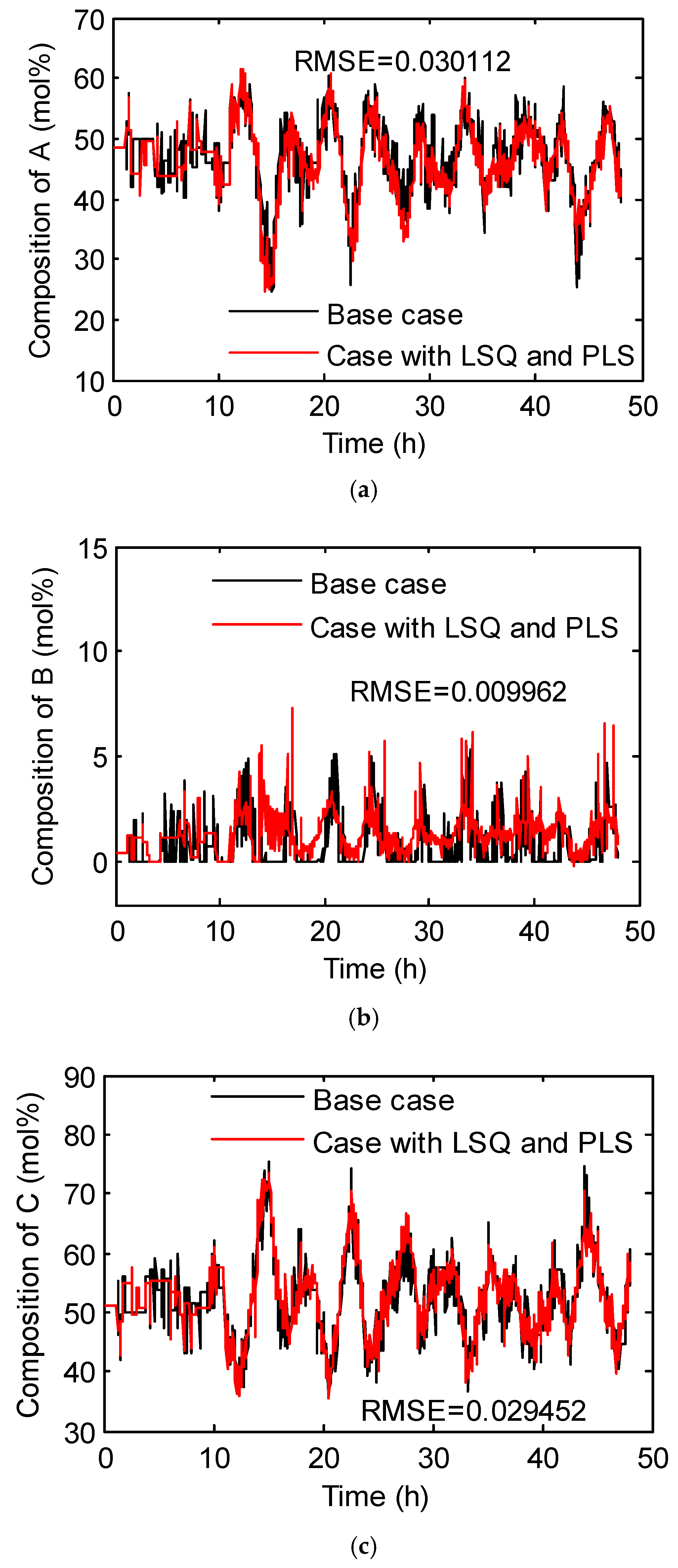
3.3. Hybrid Inverse Problem-Solving Strategy

In the above sections, two kinds of improvements—increasing the prediction accuracy of initial values and decreasing the number of iterations—were conducted for the least squares algorithm. The computational results show that the latter has a significant effect on the fault diagnosis speed. Generally, these algorithms use the passive trial and error method to solve the inverse problem of fault diagnosis. Fault parameters are defined as input variables for the system model used by LSQ, different from their output variable role defined in the inverse problem. In the following, an alternative inverse problem model using a direct mapping of fault parameters from measurements will be considered to avoid the time-consuming model solving process.

In an information view of fault diagnosis, the inverse problem defined herein is a typical multiple input-multiple output (MIMO) system in which measurable/controllable variables and fault parameters constitute input and output parts, respectively. The linear MIMO model is given by the PLS method in this work owing to the small data change for both input and output variables in a short sampling interval. Furthermore, periodic correction for this linear model by LSQ is necessary to preserve its accuracy.

Figure 10 shows the comparison of fault diagnosis for the base case and the case using a hybrid strategy. It proves the feasibility and accuracy of this strategy, but indicates larger fluctuations of the fault parameter with the hybrid algorithm. Therefore, PLS is suitable for replacing LSQ, but its application should be controlled properly. Factors affecting the efficiency of this strategy will be discussed hereafter.

(1) Number of PLS components

PLS is something of a cross between multiple linear regression and principal component analysis. It constructs components as linear combinations of the original variables, while allowing for correlation between independent and dependent variables. The number of components is therefore of primary importance to the accuracy of the PLS model. Figure 11 depicts the percent of variance explained in the dependent variable as a function of the component number. A maximum of 16 components is assumed in Figure 11 because the independent variables consist of a total of 16 variables for the stripper in TEP. It can be seen that more than 95 percent variance was explained by the first three components, which were, accordingly, chosen as the principle components in the following PLS modeling process.

(2) Sampling data set for PLS modeling

The training data sets for PLS modeling were composed of 12 measured variables, 4 manipulated variables, and 1 fault parameter. As shown in Figure 1, the fault parameter may be obtained from LSQ or PLS, so the PLS model can be built on LSQ-generated fault parameter sets (Vector I) or mixed sets (Vector II).

Figure 12a,b show the fault diagnosis results with Vector II as training data sets for PLS, whereas Figure 12c,d give results with Vector I as training data sets. The root mean square error (RMSE) of fault parameters between the base case and the proposed approach was also calculated and adhered to Figure 12a–d. As illustrated in Figure 1, a second PLS (PLS II) was performed with the aim of keeping the continuity of fault parameters when no abnormal signals were detected. Figure 12 shows the fault parameters obtained with (b) and without (a) in this second PLS based on Vector II. The worse result obtained with PLS than without PLS to predict the fault parameter in normal states evidences an adverse propagation effect of PLS prediction error on the PLS model itself. The fact that diagnosis results with Vector I as training data sets for PLS coincide exactly with the base case no matter whether they are with (d) or without (c) the second PLS further proves this conclusion. Consequently, PLS modeling should be conducted based on the fault parameters generated by the LSQ algorithm to preserve its accuracy.

Generally, the time-saving prediction of fault parameters with the PLS method may be equal to several sampling periods before each time-consuming LSQ in Figure 1. Although this scheme can cut down the running time of fault diagnosis greatly, the using frequency of PLS should be limited to an allowable range since the PLS accuracy strongly depends on new fault parameters generated by LSQ. In other words, it is crucial to correct the PLS model with LSQ-generated data after consecutive calls of PLS.

Figure 13 shows the effect of the correction interval on QFE, the running time, and RMSE, respectively. We can see from Figure 13a,b that QFE decreases, as does the running time of the fault diagnosis process, when increasing the correction interval. In particular, their decreasing magnitude becomes small when the correction interval exceeds 5. However, there appears to be a rapid growth of calculation error, as can be seen from Figure 13c. Although the effect of correction interval 4 or 5 on RMSE is not significant, both QFE and the running time will increase for the correction interval of 4 compared with 5. Therefore, 5 is the appropriate calling number of PLS in a correction interval. With this calling number, QFE decreases by 81.60% and the running speed increases about 1.7 times compared to the base case with this calling number.

Table 1. Algorithm improvement concerning function evaluations.

No.	Improvement Approach	Quantity of Function Evaluations	Cut Ratio (%)
0	base case	1826	-
1	linearly fitted initial values	1790	1.97
2	initial values provided with grey model	1740	4.71
3	one iteration only	816	55.31
4	partial least squares (PLS) mixed algorithm	336	81.60

summarizes the approaches that can effectively reduce QFE in fault diagnosis. The best results obtained are indicated in boldface. It leads to the conclusion that the approach proposed in this paper evaluates the fault parameter markedly faster than the pure LSQ-based algorithm used in [16].

The above feasibility test was implemented based on a step-type fault, with fault 7 as an example. Next, another type of fault, a random type with fault 8 as an example, will be tested with the aforementioned hybrid structure. In the case of fault 8, the composition of the feed stream (containing component A, B, and C only) changes randomly from the 8 h point. The essentially random sampling values form this fault are fed to the hybrid fault diagnosis algorithm as a preset input from an outside battery. It is satisfactory to discriminate the fault type from fault diagnosis results, with no need for a statistics analysis of random sampling values. Its fault diagnosis result with LSQ only is shown in Figure 14 and Figure 15, also published in our early work [16]. The overall running time and QFE for this diagnosis process are 5103 seconds and 19,256, respectively. This case is referred to as the base case for fault 8 in the following discussions.

Similar to Figure 11, Figure 16 shows the percent of variance explained by independent components. The first two components make more than 80% contributions and were thus selected as the components in PLS modeling under fault 8.

Figure 17 shows the effect of the correction interval on QFE (a), the running time (b), and RMSE (c) under fault 8. We can see that QFE and the running time decrease, but RMSE increases, when increasing the correction interval. 5 is chosen as the optimal correction interval since the former two indices do not decrease significantly, while RMSE remains small under this choice. Besides, larger values of the former two indices than fault 7 are observed in Figure 17, indicating that a random-type fault consumes more time than a step-type fault due to its stochastic computing load.

With 5 as the correction interval, the diagnosis result of three compositions in the bottom feed of the stripper is shown in Figure 18. It indicates nearly the same composition trajectories for the hybrid approach and base case, and proves the feasibility and accuracy of our proposed approach. Finally, QFE decreases by 92.31% and the running speed increases about 13 times compared to the base case in this situation.

4. Conclusions

In this paper, an LSQ and PLS combined hybrid inverse problem approach has been proposed to realize model-based diagnosis for the distillation process. LSQ is used to identify parameters that best-represent an abnormal state of distillation on the basis of a nonlinear dynamic model. PLS regression is then used to fit these parameters with input/output signals and forecast their developing trajectories. The correction interval of PLS significantly affects the speed and accuracy of the fault diagnosis process. The approach has been carried out to successfully identify stripper-related faults in the TEP benchmark process. For fault 7, QFE decreases by 81.60% and the running speed increases about 1.7 times compared to the base case. For fault 8, QFE decreases by 92.31% and the running speed increases about 13 times compared to the base case. Therefore, it has been proven to be a computationally efficient scheme for model-based diagnosis. In conclusion, compared with a single nonlinear LSQ-based approach, the presented hybrid inverse problem approach enables a trade-off between accurate LSQ and fast PLS and is more suitable for real-time fault diagnosis.

In the future, it would be helpful to combine this approach with some process history-based approaches, like a bond graph [25], to enhance its vital ability to locate fault-specific sections prior to fault diagnosis.

References

1. Jlassi, I.; Estima, J.O.; El Khil, S.K.; Bellaaj, N.M.; Cardoso, A.J.M. A Robust Observer-Based Method for IGBTs and Current Sensors Fault Diagnosis in Voltage-Source Inverters of PMSM Drives. IEEE Trans. Ind. Appl. 2017, 53, 2894–2905. [Google Scholar] [CrossRef]
2. Sun, S.; Wei, X.; Zhang, H.; Karimi, H.R.; Han, J. Composite fault-tolerant control with disturbance observer for stochastic systems with multiple disturbances. J. Franklin Inst. 2018, 355, 4897–4915. [Google Scholar] [CrossRef]
3. Ge, H.; Yue, D.; Xie, X. Observer-Based Fault Diagnosis of Nonlinear Systems via an Improved Homogeneous Polynomial Technique. Int. J. Fuzzy Syst. 2017, 20, 403–415. [Google Scholar] [CrossRef]
4. Power, Y.; Bahri, P.A. A two-step supervisory fault diagnosis framework. Comput. Chem. Eng. 2004, 28, 2131–2140. [Google Scholar] [CrossRef]
5. Mahmoud, H.; Abdallh, A.A.; Bianchi, N.; El-Hakim, S.M.; Shaltout, A.; Dupre, L. An Inverse Approach for Interturn Fault Detection in Asynchronous Machines Using Magnetic Pendulous Oscillation Technique. IEEE Trans. Ind. Appl. 2016, 52, 226–233. [Google Scholar] [CrossRef]
6. Tian, W.; Sun, S.; Guo, Q. Fault detection and diagnosis for distillation column using two-tier model. Can. J. Chem. Eng. 2013, 91, 1671–1685. [Google Scholar] [CrossRef]
7. Yu, H.; Khan, F.; Garaniya, V. Nonlinear Gaussian Belief Network based fault diagnosis for industrial processes. J. Process Control 2015, 35, 178–200. [Google Scholar] [CrossRef]
8. Díaz, C.A.; Echevarría, L.C.; Prieto-Moreno, A.; Neto, A.J.S.; Llanes-Santiago, O. A model-based fault diagnosis in a nonlinear bioreactor using an inverse problem approach and evolutionary algorithms. Chem. Eng. Res. Des. 2016, 114, 18–29. [Google Scholar] [CrossRef]
9. Lyu, T.; Xu, C.; Chen, G. Health state inversion of Jack-up structure based on feature learning of damage information. Eng. Struct. 2019, 186, 131–145. [Google Scholar] [CrossRef]
10. Ramos, A.R.; de Lazaro, J.M.B.; Prieto-Moreno, A. An approach to robust fault diagnosis in mechanical systems using computational intelligence. J. Intell. Manuf. 2019, 30, 1601–1615. [Google Scholar] [CrossRef]
11. Echevarría, L.C.; Velho, H.F.d.; Becceneri, J.C.; Neto, A.J.d.; Santiago, O.L. The fault diagnosis inverse problem with Ant Colony Optimization and Ant Colony Optimization with dispersion. Appl. Math. Comput. 2014, 227, 687–700. [Google Scholar] [CrossRef]
12. Parolin, R.d.S.; Neto, A.J.d.S.; Rodrigues, P.P.G.W.; Santiago, O.L. Estimation of a contaminant source in an estuary with an inverse problem approach. Appl. Math. Comput. 2015, 260, 331–341. [Google Scholar] [CrossRef]
13. Tarokh, M. Solving inverse problems by decomposition, classification and simple modeling. Inf. Sci. 2013, 218, 51–60. [Google Scholar] [CrossRef]
14. Sever, A. A neural network algorithm to pattern recognition in inverse problems. Appl. Math. Comput. 2013, 221, 484–490. [Google Scholar] [CrossRef]
15. Deshpande, A.P.; Patwardhan, S.C. Online Fault Diagnosis in Nonlinear Systems Using the Multiple Operating Regime Approach. Ind. Eng. Chem. Res. 2008, 47, 6711–6726. [Google Scholar] [CrossRef]
16. Tian, W.; Guo, Q.; Sun, S. Dynamic simulation based fault detection and diagnosis for distillation column. Korean J. Chem. Eng. 2012, 29, 9–17. [Google Scholar] [CrossRef]
17. Yin, S.; Zhu, X.; Kaynak, O. Improved PLS focused on key-performance-indicator-related fault diagnosis. IEEE Trans. Ind Electron. 2015, 62, 1651–1658. [Google Scholar] [CrossRef]
18. Vitale, R.; Palaci-Lopez, D.; Kerkenaar, H.H.M. Kernel-Partial Least Squares regression coupled to pseudo-sample trajectories for the analysis of mixture designs of experiments. Chemom. Intell. Lab. Syst. 2018, 175, 37–46. [Google Scholar] [CrossRef] [Green Version]
19. Choi, S.W.; Lee, I.-B. Multiblock PLS-based localized process diagnosis. J. Process Control 2005, 15, 295–306. [Google Scholar] [CrossRef]
20. Zhang, Y.W.; Zhou, H.; Qin, S.J.; Chai, T.Y. Decentralized fault diagnosis of large-scale processes using multiblock kernel partial least squares. IEEE Trans. Ind. Inf. 2010, 60, 3–10. [Google Scholar] [CrossRef]
21. Godoy, J.L.; Vega, J.R.; Marchetti, J.L. A fault detection and diagnosis technique for multivariate processes using a PLS-Decomposition of the measurement space. Chemom. Intell. Lab. Syst. 2013, 128, 25–36. [Google Scholar] [CrossRef]
22. Downs, J.J.; Vogel, E.F. A plant-wide industrial process control problem. Comput. Chem. Eng. 1993, 17, 245–255. [Google Scholar] [CrossRef]
23. Kayacan, E.; Ulutas, B.; Kaynak, O. Grey system theory-based models in time series prediction. Expert Syst. Appl. 2010, 37, 1784–1789. [Google Scholar] [CrossRef]
24. Tserng, H.P.; Tserng, T.L.; Chen, P.C.; Tran, L.Q. A Grey System Theory-Based Default Prediction Model for Construction Firms. Comput.-Aided Civ. Infrastruct. Eng. 2015, 30, 120–134. [Google Scholar] [CrossRef]
25. Yu, M.; Xiao, C.Y.; Jiang, W.H.; Yang, S.L.; Wang, H. Fault diagnosis for electromechanical system via extended analytical redundancy relations. IEEE Trans. Ind. Inf. 2018, 14, 5233–5244. [Google Scholar] [CrossRef]
Figure 1. Hybrid inverse problem-solving process for fault diagnosis.
Processes 08 00055 g001
Figure 2. Correction framework of partial least squares (PLS) by least squares (LSQ).
Processes 08 00055 g002
Figure 3. Fault parameter in the base case of fault 7.
Processes 08 00055 g003
Figure 4. Function evaluation in the base case of fault 7.
Processes 08 00055 g004
Figure 5. Fault diagnosis of fault 7 with linear fitted initial values.
Processes 08 00055 g005
Figure 6. Fault diagnosis of fault 7 with parabola fitted initial values.
Processes 08 00055 g006
Figure 7. Fault diagnosis of fault 7 with grey model-predicted initial values.
Processes 08 00055 g007
Figure 8. Fault diagnosis of fault 7 with different numbers of iterations.
Processes 08 00055 g008
Figure 9. Fault diagnosis of fault 7 with one iteration only.
Processes 08 00055 g009
Figure 10. Fault diagnosis of fault 7 with the hybrid algorithm.
Processes 08 00055 g010
Figure 11. Number analysis of PLS components under fault 7.
Processes 08 00055 g011
Figure 12. Fault diagnosis under fault 7 (a) based on Vector II data, but without second PLS; (b) based on Vector II data and with second PLS; (c) based on Vector I data, but without second PLS; (d) based on Vector I data and with second PLS.
Processes 08 00055 g012aProcesses 08 00055 g012b
Figure 13. Fault diagnosis with different correction intervals of PLS under fault 7 with respect to (a) quantity of function evaluations (QFE); (b) the running time; (c) the root mean square error (RMSE).
Processes 08 00055 g013
Figure 14. Fault parameter in the base case of fault 8.
Processes 08 00055 g014
Figure 15. Function evaluation in the base case of fault 8.
Processes 08 00055 g015
Figure 16. Number analysis of PLS components under fault 8.
Processes 08 00055 g016
Figure 17. Fault diagnosis with different correction intervals of PLS under fault 8 with respect to (a) QFE; (b) the running time; (c) RMSE.
Processes 08 00055 g017
Figure 18. Fault diagnosis with a hybrid scheme under fault 8 for the (a) composition of A; (b) composition of B; (c) composition of C.
Processes 08 00055 g018