Nonlinear Structural Control Analysis of an Offshore Wind Turbine Tower System

Abstract

This paper investigates the vibration control, stability, and energy transfer of the offshore wind turbine tower system with control force and nonlinearity terms. A nonlinear proportional derivative (NPD) controller was connected to the system to reduce a high oscillation amplitude and to transfer the energy in the wind turbine system. Furthermore, the averaging method and Poincaré maps were used with respect to the controlled system to study the stability and bifurcation analysis in the worst resonance cases. The curves of force response and frequency response were plotted before and after the control unit was added to the wind turbine system. In addition, we discuss the performances of the control parameters on the vibration magnitudes. Numerical simulations were carried out with Maple and Matlab algorithms to confirm the analytical results. The results show the effectiveness of the NPD controller in suppressing the nonlinear oscillations of the wind turbine system.

1. Introduction

In recent decades, renewable energy has been constantly increasing on a worldwide scale. The production of wind energy is considered one of the most cost-effective projects [1,2]. Vibration isolation and the effect of earthquake forces on behavior have been investigated for the structures of wind turbines. Moreover, the effect of parameters on the response of the turbine structure, including the blades, has been studied, and the responses were simulated using the finite element method [3]. The approach of active fault-tolerant control with “added value” as a fault tolerant system was applied to enhance the sustainability of a wind turbine in an offshore environment [4]. The technique of passive control with tuned mass dampers was used to mitigate the oscillations of spars and offshore wind turbine nacelles [5]. The active control influences on a floating wind turbine were examined and studied [6]. Mathematical analysis, uniqueness, existence, and simulations of the multi-time scale for wind turbines dynamics under control limits were studied [7]. Active tuned mass dampers were proposed to improve the accuracy of wind turbine towers [8]. Numerical simulations were performed to evaluate the dynamics of an offshore wind turbine tower with two different approaches [9]. The dynamic behavior was investigated for the inclined cable resonance under harmonic excitation [10]. The passive control approach was performed to study system behavior under multiple types of excitation forces [11,12,13]. The stability, bifurcation analyses using the averaging method, the Poincaré maps of a Cartesian manipulator system, and the energy transfer of a micro-electromechanical (MEMS) gyroscope system were studied [14,15]. A PD control unit was proposed at primary resonance to suppress the system vibrations of a horizontally supported Jeffcott-rotor. In addition, the effects of the time-delays and control gains on the system response were studied. It was reported that the optimal feedback controls are the positive-position and negative-velocity. [16,17]. Analysis details of some dynamical systems with different forces have been found [18,19]. In the present work, the nonlinear proportional derivative (NPD) controller was connected to the system to reduce a high oscillation amplitude and to transfer the energy in the wind turbine system. The averaging method and Poincaré maps were used with respect to the controlled system to study the stability and bifurcation analysis in the worst resonance cases. Additionally, the curves of force response and frequency response were plotted before and after the control unit was added to the wind turbine system

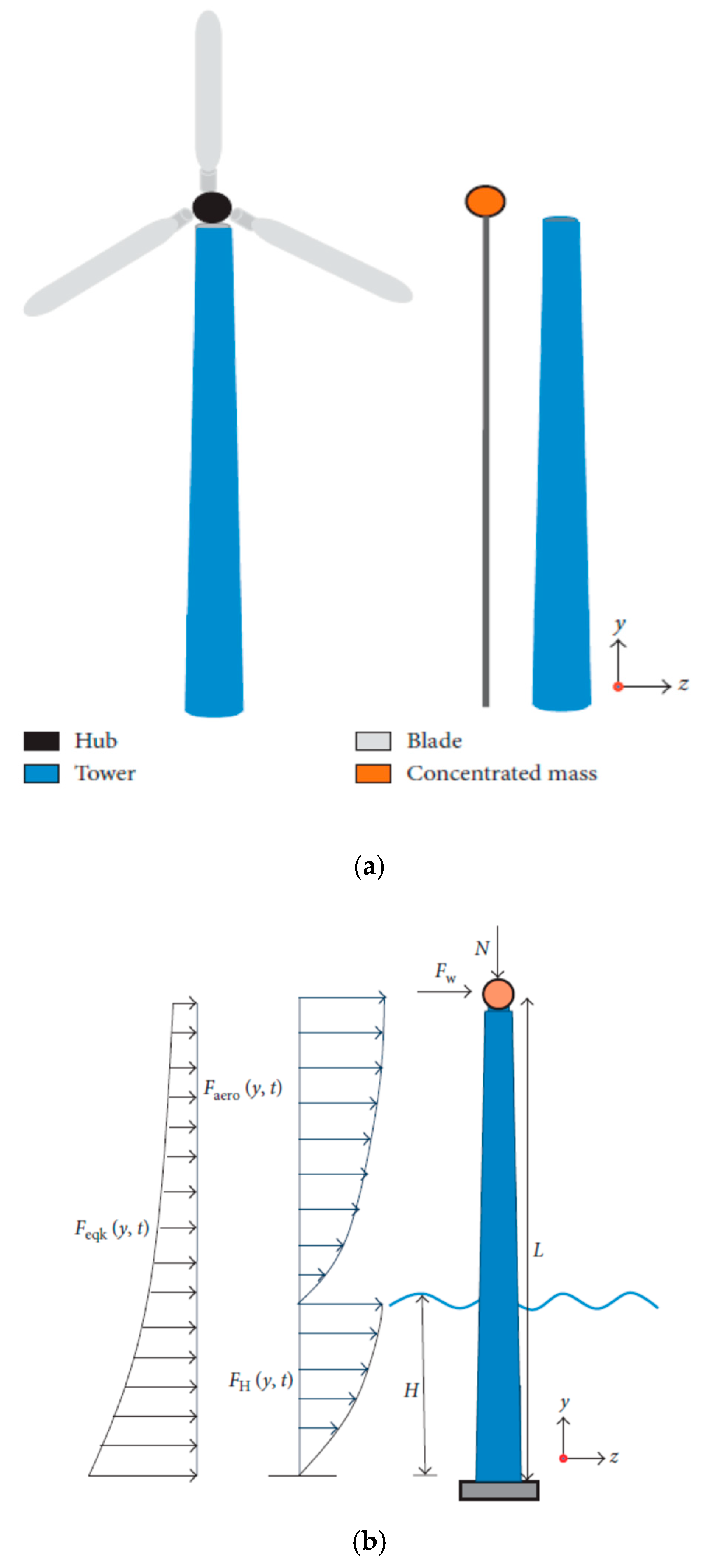
2. System Modeling

The offshore wind turbine tower system consists of a hub, tower, blade, and concentrated mass. A model of the offshore wind turbine tower is presented in Figure 1a. The height of the hub is 65 m with a diameter of 6 m, the blade length is 24 m, and the tower carries the weight of the hub, the nacelle, and the rotor blades, which is 83,000 kg. The structural modal subjected to parametric (base excitation) force $F_1$ (force multiplied by displacement) and some external forces such as wind force $F_{aero},$ wave force $F_H,$ and earthquake force $F_{eqk}$ as shown in Figure 1b.

The equation of the motion of the single degree of freedom system was obtained from [9] and is described by the following equations:

$$m\ddot{z}\left(t\right)+\epsilon c\dot{z}\left(t\right)+kz\left(t\right)+\epsilon F\left(t\right)=\epsilon G\left(t\right)$$

(1a)

where $z\left(t\right)$ is the coordinate vector, $\dot{z}\left(t\right)$ is the velocity, $\ddot{z}\left(t\right)$ is the acceleration, $G\left(t\right)$ is the signal controller, $F\left(t\right)$ is the total force, $m$ is the mass, and $c$ and $k$ are the coefficients of damping and stiffness, respectively.

$$\mathrm{Let}\{\begin{array}{l}z=u_1\hfill \\ \dot{z}={\dot{u}}_1=u_2\hfill \\ \ddot{z}={\ddot{u}}_1={\dot{u}}_2\hfill \end{array}.$$

(1b)

Equation (1a) is written in the matrix form as

$$\begin{array}{c}\left(\begin{array}{l}{\dot{u}}_1\hfill \\ {\dot{u}}_2\hfill \end{array}\right)=\left(\begin{array}{ll}0\hfill & 1\hfill \\ -{\omega }^2-\epsilon {\alpha }_2{u}_2^2+\epsilon f_1{\cos \mathsf{\Omega }}_{1}t\hfill & -\epsilon \mu -\epsilon {\alpha }_1{u}_1^2\hfill \end{array}\right)\left(\begin{array}{l}{u}_1\hfill \\ u_2\hfill \end{array}\right)\\ +\left(\begin{array}{l}0\hfill \\ -\epsilon \alpha \cos \pi t-\epsilon f_a\sin \mathsf{\Omega }t+\epsilon f_H\cos \mathsf{\Omega }t\left|\cos \mathsf{\Omega }t\right|\hfill \end{array}\right)\end{array}$$

(1c)

where $\mu =\frac{c}{m}, {\omega }^2=\frac{k}{m}, F\left(t\right)=\frac{1}{m}\left(F_{eqk}+F_{aero}\sin \mathsf{\Omega }t-\epsilon F_{H }\cos \mathsf{\Omega }t \left|\cos \mathsf{\Omega }t\right|-F_1\right),$ and $G\left(t\right)=\left(-{\alpha }_1{u}^2\dot{u}-{\alpha }_{2}u{\dot{u}}^2\right).$

The initial conditions of Equation (1) are as follows: $u\left(0\right)=0.01, \dot{u}\left(0\right)=0.01,$ $\mu$ is the linear damping coefficient, $\epsilon$ is the small perturbation, $f_a\mathrm{and}{f}_H$ are the wind and wave excitation forces, $F_{eqk}=\alpha \cos \pi t$ is the earthquake force, $F_1=f_{1}u {\cos \mathsf{\Omega }}_{1}t$ is the parametric force, $\omega$ is the natural frequency, $\mathsf{\Omega }$ and ${\mathsf{\Omega }}_1$ are the excitation frequencies, and $\left(-{\alpha }_1{u}^2\dot{u}-{\alpha }_{2}u{\dot{u}}^2\right)$ refers to the nonlinear proportional-derivative (NPD) controller.

2.1. The Averaging Method

The averaging method [20,21] is applied for Equation (1) to obtain the frequency response equations. When $\epsilon =0,$ Equation (1c) can be written as

$${\ddot{u}}_1+{\omega }^2{u}_1=0.$$

(2a)

The solution of Equation (2a) is expressed as

$$u_1=a\cos \left(\omega t+\phi \right)$$

(2b)

where $a$ and $\phi$ are the free integration constants, and $\omega$ is also constant. It follows from Equation (2b) that

$${\dot{u}}_1=u_2=-\omega a\sin \left(\omega t+\phi \right)$$

(3)

where, if $\epsilon \ne 0$ is small enough, $a$ and $\phi$ are functions in time $t$ for Equation (1c).

Therefore, Equation (2b) is differentiated with time $t$ yields:

$${\dot{u}}_1=u_2=\dot{a}\cos \left(\omega t+\phi \right)-\omega a\sin \left(\omega t+\phi \right)-a\dot{\phi }\sin \left(\omega t+\phi \right).$$

(4)

Comparing Equation (3) and Equation (4), we conclude that

$$\dot{a}\cos \left(\omega t+\phi \right)-a\dot{\phi }\sin \left(\omega t+\phi \right)=0.$$

(5)

Differentiating Equation (3) once with respect to $t,$ we have

$${\ddot{u}}_1={\dot{u}}_2=-\omega \dot{a}\sin \left(\omega t+\phi \right)-{\omega }^{2}a\cos \left(\omega t+\phi \right)-\omega a\dot{\phi }\cos \left(\omega t+\phi \right).$$

(6)

Inserting $u_1, {\dot{u}}_1,$ and ${\ddot{u}}_1$ from Equations (2)–(6) into Equation (1c), we obtain

$$\begin{array}{c}-\dot{a}\omega \sin \left(\omega t+\phi \right)-a\dot{\phi }\omega \cos \left(\omega t+\phi \right)-\epsilon \mu \omega \mathrm{asin}\left(\omega t+\phi \right)+\epsilon f_a\sin \left(\mathsf{\Omega } t\right)\\ +\epsilon \alpha \cos \left(\pi t\right)-\epsilon f_H{\cos }^2\left(\mathsf{\Omega } t\right)-\frac{\epsilon f_{1}a}{2}\left(\cos \left(\left(\mathsf{\Omega }+\omega \right)t+\phi \right)+\cos \left(\left(\mathsf{\Omega }-\omega \right)t-\phi \right)\right)\\ -\frac{\epsilon {\alpha }_1\omega a^3}{4}\left(\sin \left(\omega t+\phi \right)+\sin \left(3\omega t+3\phi \right)\right)-\frac{\epsilon {\alpha }_2{\omega }^2{a}^3}{2}\left(\cos \left(\omega t+\phi \right)-\cos \left(3\omega t+3\phi \right)\right)=0.\end{array}$$

(7)

Substituting Equation (5) in Equation (7) and solving it for $\phi$ and $a$ yields

$$\begin{array}{c}\dot{a}=-\frac{\epsilon \mu a}{2}\left(1-\cos \left(2\omega t+2\phi \right)\right)-\frac{\epsilon f_{1}a}{4\omega }\left\{\sin \left[\left({\mathsf{\Omega }}_1+2\omega \right)t+2\phi \right]-\sin \left[\left({\mathsf{\Omega }}_1-2\omega \right)t-2\phi \right]\right\}\\ -\frac{\epsilon {\alpha }_1{a}^3}{8}\left(1-\cos \left(4\omega t+4\phi \right)\right)-\frac{\epsilon f_a}{2\omega }\left\{\cos \left[\left(\mathsf{\Omega }+\omega \right)t+\phi \right]-\cos \left[\left(\mathsf{\Omega }-\omega \right)t-\phi \right]\right\}\\ +\frac{\epsilon \alpha }{2\omega }\left\{\sin \left[\left(\pi +\omega \right)t+\phi \right]-\sin \left[\left(\pi -\omega \right)t-\phi \right]\right\}-\frac{\epsilon {\alpha }_2\omega a^3}{8}\left\{\sin \left(4\omega t +4\phi \right)-2\sin \left(2\omega t +2\phi \right)\right\}\\ -\frac{\epsilon f_H}{4\omega }\left\{\sin \left[\left(2\mathsf{\Omega }+\omega \right)t+\phi \right]-\sin \left[\left(2\mathsf{\Omega }-\omega \right)t-\phi \right]+2\sin \left(\omega t +\phi \right)\right\}\end{array}$$

(8)

$$\begin{array}{c}a{\dot{\phi }}_1=-\frac{\epsilon \mu a}{2}\sin \left(2\omega t+2\phi \right)\\ -\frac{\epsilon f_{1}a}{4\omega }\left\{\cos \left[\left({\mathsf{\Omega }}_1+2\omega \right)t+2\phi \right]+\cos \left[\left({\mathsf{\Omega }}_1-2\omega \right)t-2\phi \right]+2\cos \left({\mathsf{\Omega }}_{1}t\right)\right\}\\ -\frac{\epsilon {\alpha }_1{a}^3}{8}\left\{\sin \left(4\omega t +4\phi \right)+2\sin \left(2\omega t +2\phi \right)\right\}\\ +\frac{\epsilon f_a}{2\omega }\left\{\sin \left[\left(\mathsf{\Omega }+\omega \right)t+\phi \right]+\sin \left[\left(\mathsf{\Omega }-\omega \right)t-\phi \right]\right\}\\ +\frac{\epsilon \alpha }{2\omega }\left\{\cos \left[\left(\pi +\omega \right)t+\phi \right]+\cos \left[\left(\pi -\omega \right)t-\phi \right]\right\}+\frac{\epsilon {\alpha }_2\omega a^3}{8}\left(1-\cos \left(4\omega t+4\phi \right)\right)\\ -\frac{\epsilon f_H}{4\omega }\left\{\cos \left[\left(2\mathsf{\Omega }+\omega \right)t+\phi \right]+\cos \left[\left(2\mathsf{\Omega }-\omega \right)t-\phi \right]+2\cos \left(\omega t +\phi \right)\right\}.\end{array}$$

(9)

2.2. Periodic Solutions

To find the approximate solutions of Equations (8) and (9) using the perturbation technique, we introduce detuning parameters ${\sigma }_1$ and ${\sigma }_2$ to convert the small divisor terms into secular terms at the worst resonance cases $\mathsf{\Omega }\cong \omega$ and ${\mathsf{\Omega }}_1\cong 2\omega .$ Moreover, to describe the nearness of the resonances (primary and sub-harmonic), two detuning parameters ${\sigma }_1$ and ${\sigma }_2$ were introduced and defined by ($\mathsf{\Omega }\cong \omega +\epsilon {\sigma }_1$ and ${\mathsf{\Omega }}_1\cong 2\omega +\epsilon {\sigma }_2)$ and the slowly varying parts and constant terms are only in Equations (8)–(9), so we have

$$\dot{a}=-\frac{\mu }{2}a-\frac{{\alpha }_1}{8}{a}^3+\frac{f_a}{2\omega }cos {\theta }_1+\frac{f_1}{4\omega }a sin 2{\theta }_1$$

(10)

$${\dot{\theta }}_1={\sigma }_1-\frac{{\alpha }_2 \omega }{8}{a}^2-\frac{f_a}{2a\omega }sin {\theta }_1+\frac{f_1}{4\omega }cos 2{\theta }_1$$

(11)

where ${\theta }_1={\sigma }_1{T}_1-\phi ,$ ${\theta }_2={\sigma }_2{T}_1-2\phi ,$ and ${\theta }_2=2{\theta }_1.$

2.3. Equilibrium Solutions and Stability Analyses

The steady-state solution occur where $\dot{a}={\dot{\theta }}_1=0,$ and the solutions at steady state can then be obtained as follows:

$$\frac{\mu }{2}a+\frac{{\alpha }_1}{8}{a}^3=\frac{f_a}{2\omega }cos {\theta }_1+\frac{f_1}{4\omega }a sin 2{\theta }_1$$

(12)

$$a{\sigma }_1-\frac{{\alpha }_2 \omega }{8}{a}^3=\frac{f_a}{2\omega }sin {\theta }_1-\frac{f_1}{4\omega }a cos 2{\theta }_1.$$

(13)

By squaring both sides of Equations (12) and (13) and adding the results, we obtained the frequency response equation in the form:

$${\sigma }_1^2-\left(\frac{\omega a^2{\alpha }_2}{4}\right){\sigma }_1+\left(\frac{{\mu }^2}{4}+\frac{{\alpha }_1\mu a^2}{8}+\frac{{\alpha }_1^2{a}^4}{64}+\frac{{\alpha }_2^2{\omega }^2{a}^4}{64}-\frac{f_a{}^2}{4a^2{\omega }^2}-\frac{f_1{}^2}{16{\omega }^2}\right)=0.$$

(14)

To examine the stability of the nonlinear solutions, we take

$$a=a_{10}+a_{11}\left(T_1\right)\mathrm{and}{\theta }_1={\theta }_{10}+{\theta }_{11}\left(T_1\right)$$

(15)

where $a_{10} and {\theta }_{10}$ as well as $a_{11} and {\theta }_{11}$ correspond to the nonlinear solution and perturbation terms respectively, where $a_{11} and {\theta }_{11}$ are small compared to $a_{10} and {\theta }_{10}.$ Using Equation (15) in Equations (10) and (11) and using $cos {\theta }_{11}=1$ and $sin {\theta }_{11}={\theta }_{11}$,

$$\dot{a}=\left(-\frac{\mu }{2}-\frac{3{\alpha }_1{a}_{10}^2}{8}+\frac{f_1 }{2\omega }\sin {\theta }_{10}\cos {\theta }_{10}\right) a_{11}+\left(\frac{f_1{a}_{10} }{2\omega }\cos 2{\theta }_{10}-\frac{f_a }{2\omega }\sin {\theta }_{10}\right) {\theta }_{11}$$

(16)

$${\dot{\theta }}_1=\left(\frac{f_a }{2\omega a_{10}^2}sin {\theta }_{10}-\frac{\omega {\alpha }_2{a}_{10}}{4}\right) a_{11}-\left(\frac{f_1 }{\omega }sin {\theta }_{10} cos {\theta }_{10}+\frac{f_a }{2\omega a_{10}}cos {\theta }_{10}\right) {\theta }_{11}.$$

(17)

Equations (16) and (17) can be expressed in a matrix form as follows:

$$\left[\begin{array}{l}\dot{a}\hfill \\ {\dot{\theta }}_1\hfill \end{array}\right]=\left[\begin{array}{ll}{\Gamma }_{11}\hfill & {\Gamma }_{12}\hfill \\ {\Gamma }_{21}\hfill & {\Gamma }_{22}\hfill \end{array}\right]\left[\begin{array}{l}{a}_{11}\hfill \\ {\theta }_{11}\hfill \end{array}\right]$$

(18)

where ${\mathsf{\Gamma }}_{11}=-\frac{\mu }{2}-\frac{3{\alpha }_1{a}_{10}^2}{8}+\frac{f_1 }{2\omega }\sin {\theta }_{10}\cos {\theta }_{10}, {\mathsf{\Gamma }}_{12}=\frac{f_1{a}_{10} }{2\omega }\cos 2{\theta }_{10}-\frac{f_a }{2\omega }\sin {\theta }_{10}.$

$${\Gamma }_{21}=\frac{f_a }{2\omega a_{10}^2}sin {\theta }_{10}-\frac{\omega {\alpha }_2{a}_{10}}{4}, {\Gamma }_{22}=-\frac{f_1 }{\omega }sin {\theta }_{10} cos {\theta }_{10}+\frac{f_a }{2\omega a_{10}}cos {\theta }_{10}.$$

Thus, the stability of the steady-state solutions depends on the Jacobian matrix eigenvalues of Equation (18), so the characteristic equation is obtained as

$${\lambda }^2+{\varsigma }_1\lambda +{\varsigma }_2=0$$

(19)

where the eigenvalues of the Jacobian matrix is denoted by $\lambda ,$ and ${\varsigma }_1=-\left({\mathsf{\Gamma }}_{11}+{\mathsf{\Gamma }}_{22}\right)$ and ${\varsigma }_2=\left({\mathsf{\Gamma }}_{11}{\mathsf{\Gamma }}_{22}-{\mathsf{\Gamma }}_{12}{\mathsf{\Gamma }}_{21}\right)$ are the coefficients of Equation (19). Using the criterion of Routh–Hurwitz, the necessary and sufficient conditions for the system are stable such that the real parts of all roots of Equation (19) are negative.

3. Analytical and Numerical Results

In this section, Equation (1) is integrated numerically with the fourth-order Rung–Kutta method. The effects of some different parameters on the behavior of the controlled system are also studied. Moreover, the transfer of energy between uncontrolled and controlled modes is examined. The curves of force response and frequency response are plotted before and after the control unit is added to the wind turbine system. The bifurcation analyses of the controlled system are conducted using Poincaré maps.

3.1. System Behavior and Energy Transfer in the Wind Turbine Tower System

The system behavior is studied numerically at the adopted parameter values of the controlled system: $\mu =0.04,\alpha =9.73,\mathsf{\Omega }= \omega =2.01, {\mathsf{\Omega }}_1=2 \omega ,f_a=67.17, f_H=5.129, f_1=0.002, {\alpha }_1=28,\mathrm{and}{\alpha }_2=0.5.$ The energy is transferred from the system before control to the system after adding the NPD controller at different values of resonance cases $\mathsf{\Omega }\cong \omega {\mathrm{and}\mathsf{\Omega }}_1\cong 2\omega ,$ as well as $\mathsf{\Omega }\cong 3\omega /2{\mathrm{and}\mathsf{\Omega }}_1\cong 2\omega$ as shown in Figure 2 and Figure 3, respectively. The output steady amplitude is suppressed from about 18 to about 1.5, and the control unit has an effectiveness $E_a$ equal to about 12, as shown in Figure 2. Moreover, the steady amplitude has been suppressed from about 60 to about 1.25 and has an effectiveness $E_a$ equal to about 48, as shown in Figure 3.

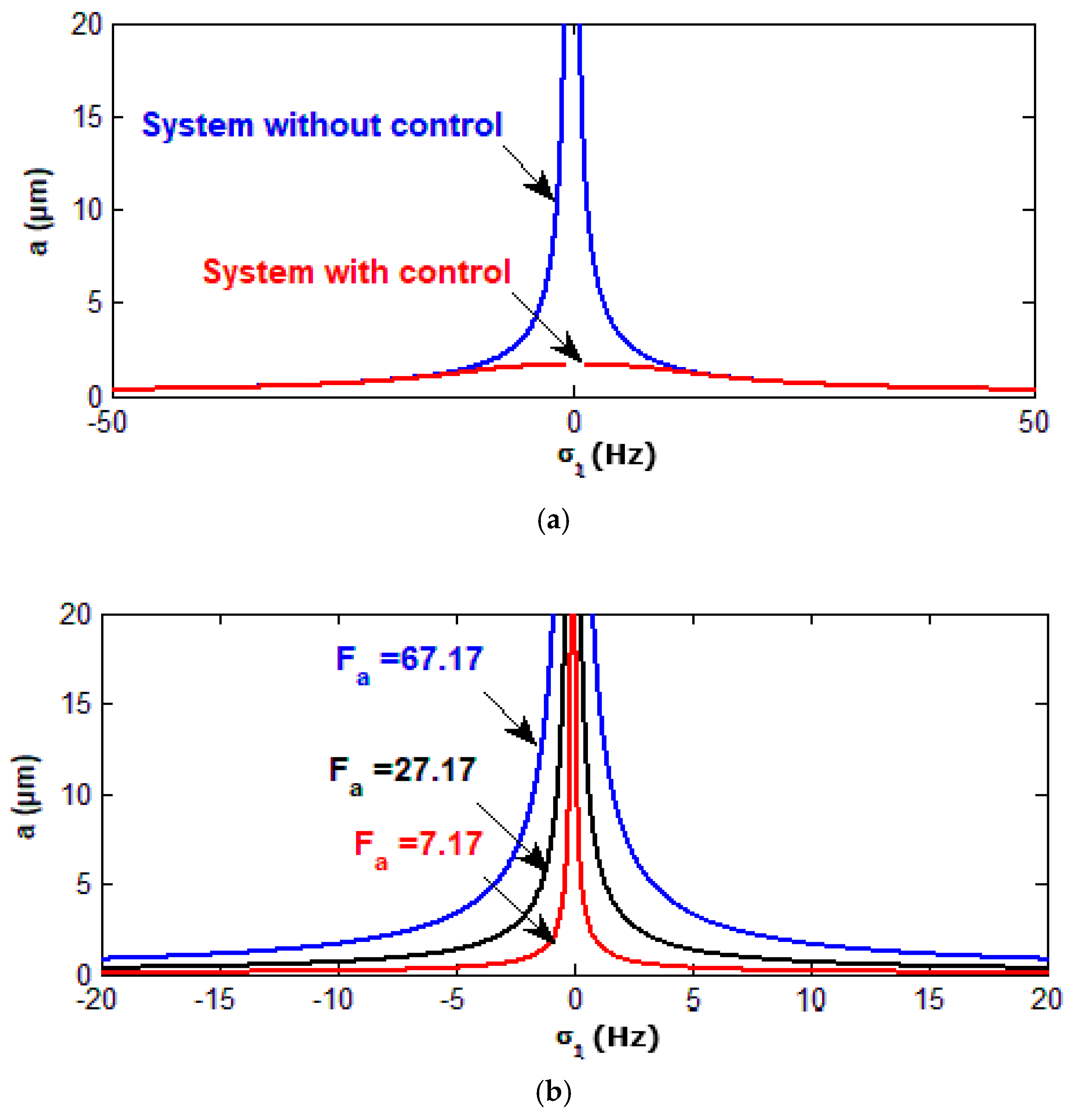
3.2. Frequency Response Curves of the Controlled System

In this section, we studied the different parameter effect and stability zone of the controlled system using frequency response curves. In Figure 4a, the detuning parameter ${\sigma }_1$ effects on the behavior of the system before and after control are shown. The controlled system behavior is a monotonic increasing function in the wind amplitude force $f_a,$ as shown in Figure 4b. However, Figure 4c shows that the behavior of the controlled system is a monotonic decreasing function in the nonlinear control parameter ${\alpha }_1,$ and the curve of the controlled system is bent to the right and the left, producing soft, hard spring, jump phenomena and multiple solutions with positive and negative values of the nonlinear control parameter ${\alpha }_2,$ respectively, as shown in Figure 4d.

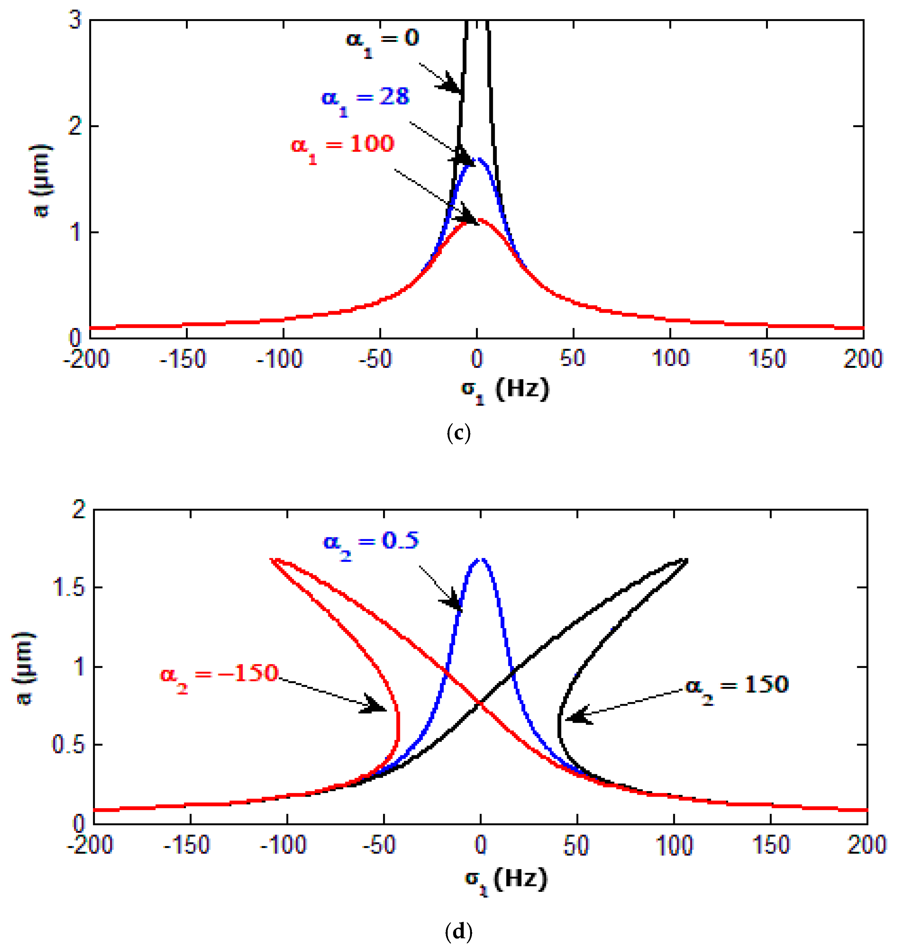
3.3. Effect of Some Different Parameters on the Controlled System

In this section, we studied the effect of some different parameters on the behavior of the controlled system at ${\sigma }_1=0.$ Figure 5a–c show that the behavior of the controlled system is a monotonic decreasing function in the control parameters ${\alpha }_1\mathrm{and}{\alpha }_2$ and the damping coefficient $\mu .$ Based on these figures, we can use these parameters for suppressing the oscillations of the wind turbine system. The behavior of the controlled system is a monotonic increasing function in the parametric excitation force $f_1,$ as shown in Figure 5d.

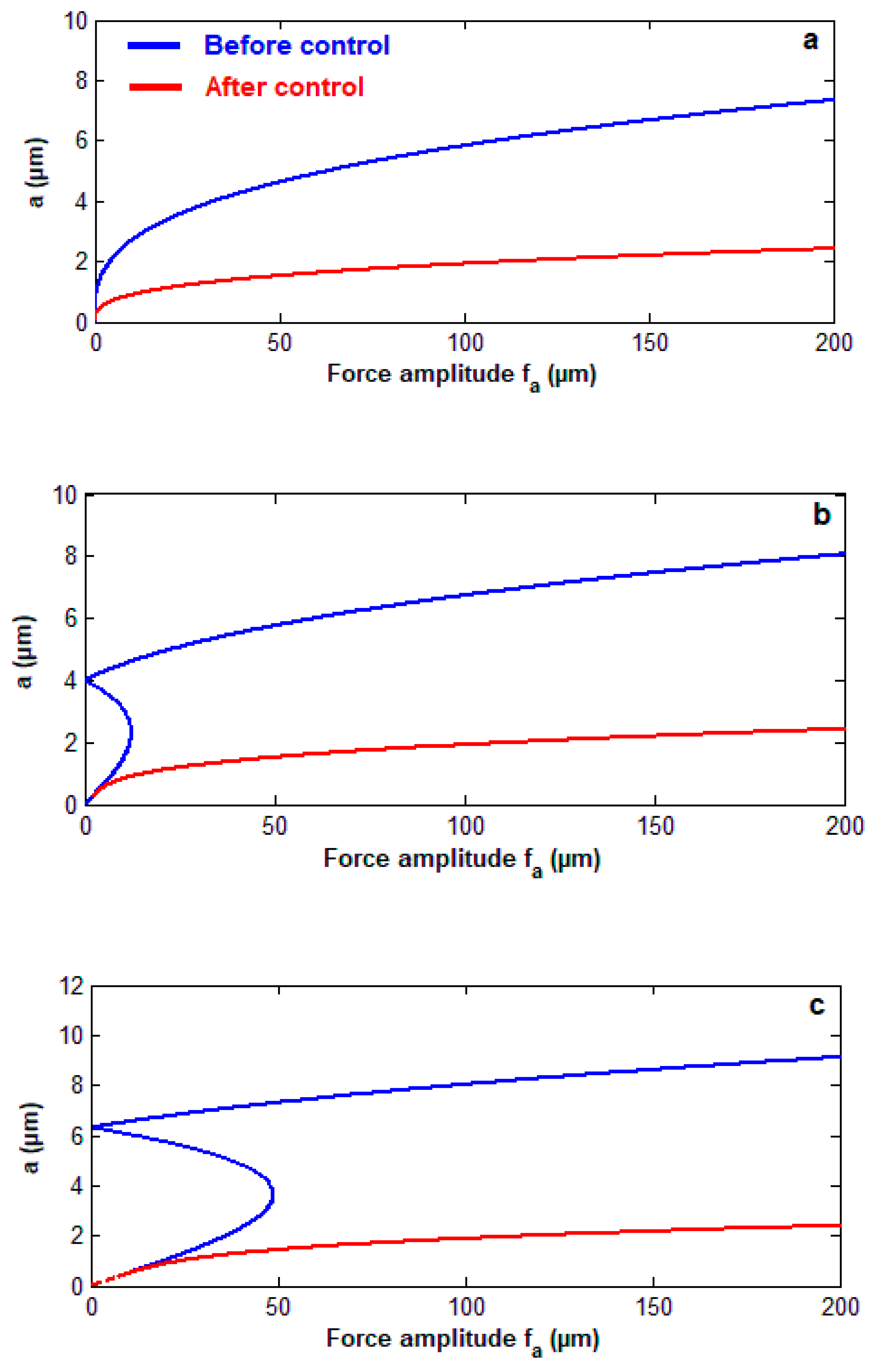
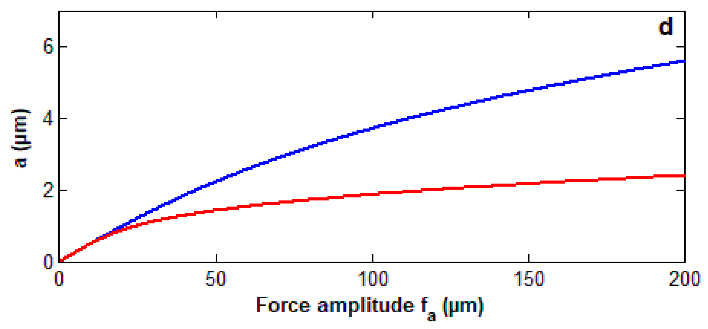
3.4. The Curves of Force Response for the Controlled System

Figure 6a–d shows the curves of force response for the controlled system at values of detuning parameter ${\sigma }_1$ before and after adding a control unit. These figures show that, for large values of $f_a,$ the system amplitude before control has a nonlinear relation with the wind turbine force, and the system has large amplitudes for a slight change in the wind turbine force. In addition, after adding a control unit, the relation becomes linear with a small slope, and the system amplitudes become less than those before control.

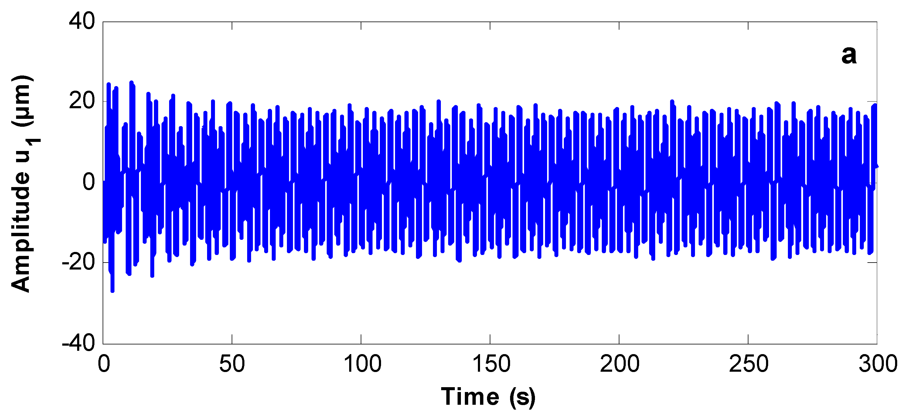
3.5. The Poincaré Maps

In this section, the stability is investigated, and bifurcation diagrams are plotted using the Poincaré maps. The complicated response in the phase space is transferred to a discrete map in the lower dimensional space using these maps. Figure 7, Figure 8 and Figure 9 show the wind turbine response at the simultaneous primary and sub-harmonic resonance case $\mathsf{\Omega }\cong \omega {\mathrm{and}\mathsf{\Omega }}_1\cong 2\omega$ with different values of gain parameters ${\alpha }_1\mathrm{and}{\alpha }_2$ with the response and Poincaré map, respectively. Figure 7a,b shows that the system starts with a chaotic response and becomes stable, and the periodic motion appears on Poincaré maps at ${\alpha }_1=0\mathrm{and}{\alpha }_2=0.$ Moreover, the system has a steady-state solution at ${\alpha }_1=28\mathrm{and}{\alpha }_2=0.5,$ as shown in Figure 8a,b. Figure 9a,b shows that the system has a quasi-periodic motion and the solution is unstable at ${\alpha }_1=0\mathrm{and}{\alpha }_2=0.5.$

3.6. Comparison with Published Work

In comparison with previous researches, Dagli et al. [9] performed the effect of environmental forces and seismic loads on the offshore wind tower behavior with a two-way (fluid–structure interaction) technique. They performed dynamic vibration analysis using Rayleigh’s energy. In addition, the single degree of freedom (SDOF) equation of motion is solved numerically using the fourth-order Runge–Kutta method.

Within this work, the authors studied the nonlinear dynamics behavior and vibration suppression of the offshore wind turbine system with multiple external and parametric excitation forces using an NPD controller. In addition, the authors investigated the energy transfer between uncontrolled and controlled system. The method of averaging is applied to analyze the response and stability of the solutions in the worst resonance cases. In the numerical results, the amplitudes have been suppressed from about 18 and 60 to about 1.5 and 1.25, respectively, and the controlled system has an effectiveness $E_a=12$ and $E_a=48.$ Moreover, jump down phenomena and multi-valued solutions appeared. Finally, the system before control becomes stable, and periodic motion appears on Poincaré maps.

4. Conclusions

The oscillations of the offshore wind turbine system were investigated with multiple external, parametric excitations with a nonlinear PD controller. The stability analysis and numerical integration were studied to determine system behavior. The effect of different parameters and force–response curves of the system were investigated before and after adding a control unit. The stability and bifurcation diagrams were studied using the Poincaré maps. From this study, we conclude the following:

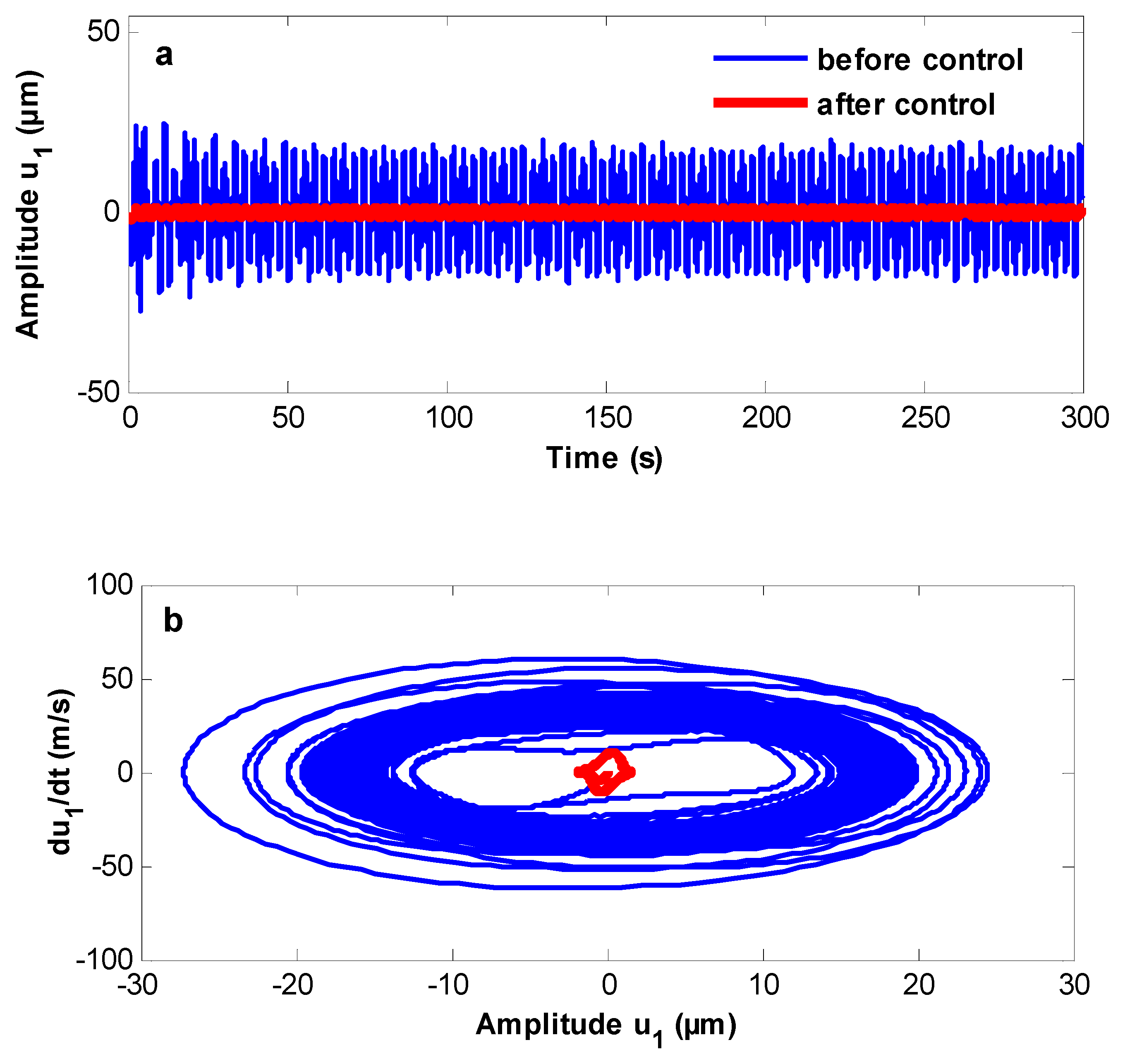
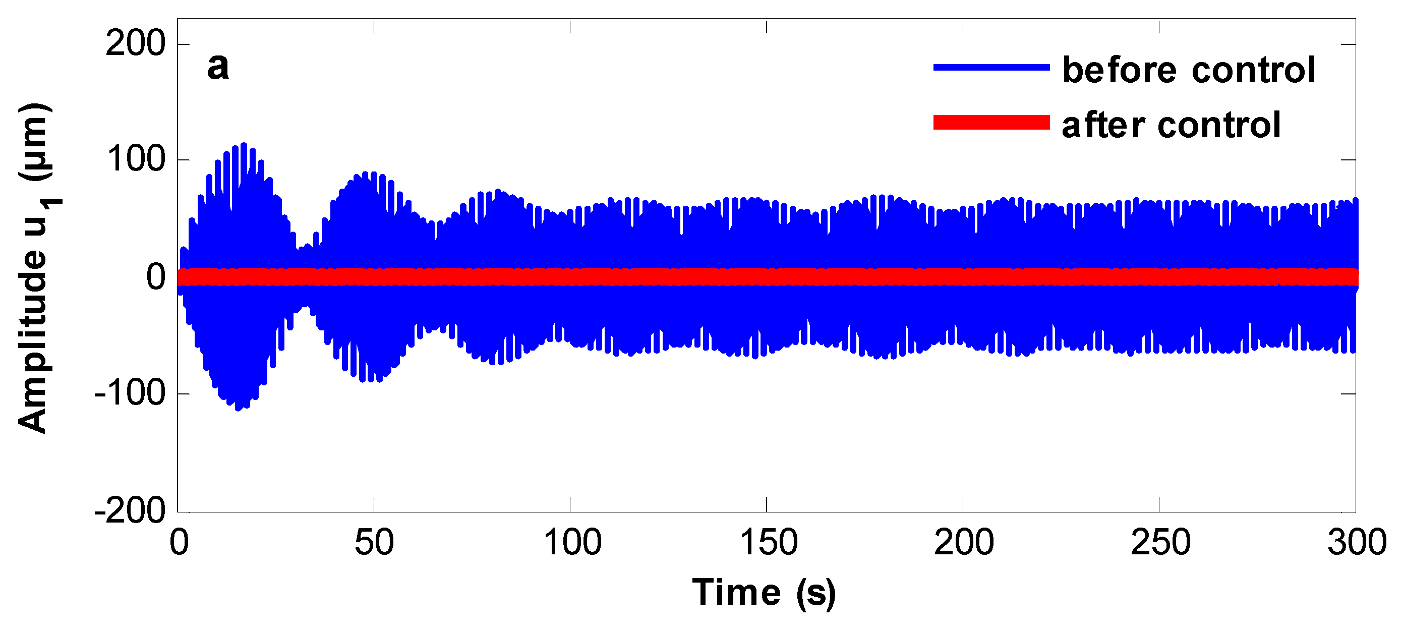
• The amplitudes were suppressed from about 18 and 60 to about 1.5 and 1.25 at resonance cases $\mathsf{\Omega }\cong \omega {\mathrm{and}\mathsf{\Omega }}_1\cong 2\omega$ as well as $\mathsf{\Omega }\cong 3\omega /2{\mathrm{and}\mathsf{\Omega }}_1\cong 2\omega ,$ respectively.
• The controlled system has an effectiveness $E_a=12$ and $E_a=48$ for the wind turbine system.
• The energy was transferred from the system before control to the system after adding the NPD controller at different values of natural, external excitation, and parametric excitation frequencies $\omega , \mathsf{\Omega },$ and ${\mathsf{\Omega }}_1$.
• The behavior of the controlled system is a monotonic increasing function of the wind amplitude force $f_a$ and the parametric excitation force $f_1,$ and is a monotonic decreasing function of the damping coefficient $\mu$ and control parameters ${\alpha }_1$ and ${\alpha }_2$.
• The controlled system has a jump phenomenon with multiple solutions for positive and negative values of the nonlinear control parameter ${\alpha }_2$.
• The system amplitude before control has a nonlinear relation and a slightly increasing amplitude for large values of $f_a,$ but it has a linear relation with small slope amplitudes after adding a controller.
• The system before control becomes stable, and periodic motion appears on Poincaré maps. The system also has a steady-state solution after control.
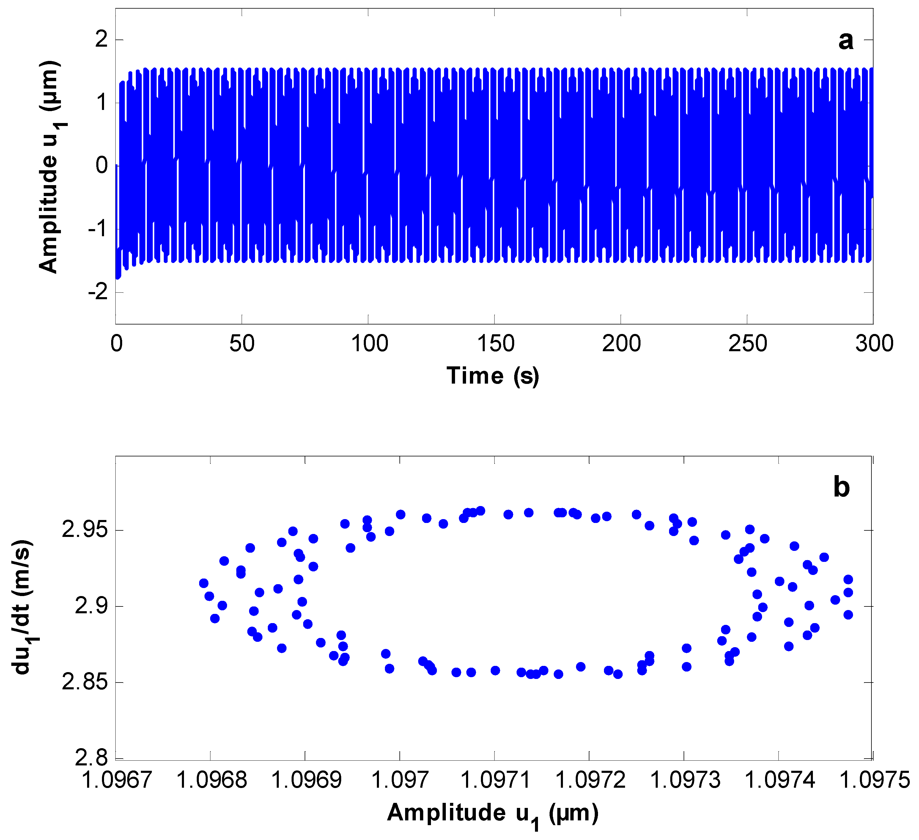
• The controlled system shows quasi-periodic motion and an unstable solution at ${\alpha }_1=0\mathrm{and}{\alpha }_2=0.5.$

References

- Silva, M.A.; Arora, J.S.; Brasil, R.M. Formulations for the optimal design of RC wind turbine towers. In Proceedings of the International Conference on Engineering Optimization (Eng Opt 2008), Rio de Janeiro, Brazil, 1–5 June 2008. [Google Scholar]
- Shi, W.; Han, J.; Kim, C.; Lee, D.; Shin, H.; Park, H. Feasibility study of offshore wind turbine substructures for southwest offshore wind farm project in Korea. Renew. Energy 2015, 74, 406–413. [Google Scholar] [CrossRef]
- Van der Woude, C.; Narasimhan, S. A study on vibration isolation for wind turbine structures. Eng. Struct. 2014, 60, 223–234. [Google Scholar] [CrossRef]
- Shi, F.; Patton, R. An active fault tolerant control approach to an offshore wind turbine model. Renew. Energy 2015, 75, 788–798. [Google Scholar] [CrossRef]
- Nguyen Dinh, V.; Basu, B. Passive control of floating offshore wind turbine nacelle and spar vibrations by multiple tuned mass dampers. Struct. Control Health Monit. 2015, 22, 152–176. [Google Scholar] [CrossRef]
- Hu, Y.; He, E. Active structural control of a floating wind turbine with a stroke-limited hybrid mass damper. J. Sound Vib. 2017, 410, 447–472. [Google Scholar] [CrossRef]
- Eisa, S.A.; Stone, W.; Wedeward, K. Mathematical analysis of wind turbines dynamics under control limits: Boundedness, existence, uniqueness, and multi time scale simulations. Int. J. Dyn. Control 2018, 6, 929–949. [Google Scholar] [CrossRef]
- Fitzgerald, B.; Sarkar, S.; Staino, A. Improved reliability of wind turbine towers with active tuned mass dampers (ATMDs). J. Sound Vib. 2018, 419, 103–122. [Google Scholar] [CrossRef]
- Dagli, B.Y.; Tuskan, Y.; Gokkus, U. Evaluation of Offshore Wind Turbine Tower Dynamics with Numerical Analysis. Adv. Civ. Eng. 2018, 2018, 3054851. [Google Scholar] [CrossRef]
- Kamel, M.M.; Hamed, Y.S. Non-Linear Analysis of an Inclined Cable under Harmonic Excitation. Acta Mech. 2010, 214, 315–325. [Google Scholar] [CrossRef]
- El-Ganaini, W.A.A.; Kamel, M.M.; Hamed, Y.S. Vibration reduction in ultrasonic machine to external and tuned excitation forces. Appl. Math. Model. 2009, 33, 2853–2863. [Google Scholar] [CrossRef]
- Kamel, M.M.; El-Ganaini, W.A.A.; Hamed, Y.S. Vibration suppression in ultrasonic machining described by non-linear differential equations. J. Mech. Sci. Technol. 2009, 23, 2038–2050. [Google Scholar] [CrossRef]
- Kamel, M.M.; El-Ganaini, W.A.A.; Hamed, Y.S. Vibration suppression in multi-tool ultrasonic machining to multi-external and parametric excitations. Acta Mech. Sinica 2009, 25, 403–415. [Google Scholar] [CrossRef]
- Hamed, Y.S.; EL-Sayed, A.T.; El-Zahar, E.R. On controlling the vibrations and energy transfer in MEMS gyroscopes system with simultaneous resonance. Nonlinear Dyn. 2016, 83, 1687–1704. [Google Scholar] [CrossRef]
- Hamed, Y.S.; Alharthi, M.R.; AlKhathami, H.K. Nonlinear vibration behavior and resonance of a Cartesian manipulator system carrying an intermediate end effector. Nonlinear Dyn. 2018, 91, 1429–1442. [Google Scholar] [CrossRef]
- Saeed, N.A.; Kamel, M. Nonlinear PD-controller to suppress the nonlinear oscillations of horizontally supported Jeffcott-rotor system. Int. J. Non Linear Mech. 2016, 87, 109–124. [Google Scholar] [CrossRef]
- Saeed, N.A.; El-Ganaini, W.A. Time-delayed control to suppress the nonlinear vibrations of a horizontally suspended Jeffcott-rotor system. Appl. Math. Model. 2017, 44, 523–539. [Google Scholar] [CrossRef]
- Cartmell, M.P. Introduction to Linear, Parametric and Nonlinear Vibrations; Chapman & Hall: London, UK, 1990. [Google Scholar]
- Nayfeh, A.H.; Balachandran, B. Applied Nonlinear Dynamics: Analytical, Computational and Experimental Methods; Wiley: New York, NY, USA, 1995. [Google Scholar]
- Nayfeh, A.H. Problems in Perturbation; Wiley: New York, NY, USA, 1985. [Google Scholar]
- Nayfeh, A.H.; Mook, D.T. Nonlinear Oscillations; Wiley: New York, NY, USA, 1995. [Google Scholar]
© 2019 by the authors. Licensee MDPI, Basel, Switzerland. This article is an open access article distributed under the terms and conditions of the Creative Commons Attribution (CC BY) license (http://creativecommons.org/licenses/by/4.0/).
Share and Cite
Hamed, Y.S.; Aly, A.A.; Saleh, B.; Alogla, A.F.; Aljuaid, A.M.; Alharthi, M.M. Nonlinear Structural Control Analysis of an Offshore Wind Turbine Tower System. Processes 2020, 8, 22. https://doi.org/10.3390/pr8010022
Hamed YS, Aly AA, Saleh B, Alogla AF, Aljuaid AM, Alharthi MM. Nonlinear Structural Control Analysis of an Offshore Wind Turbine Tower System. Processes. 2020; 8(1):22. https://doi.org/10.3390/pr8010022
Chicago/Turabian StyleHamed, Y. S., Ayman A. Aly, B. Saleh, Ageel F. Alogla, Awad M. Aljuaid, and Mosleh M. Alharthi. 2020. "Nonlinear Structural Control Analysis of an Offshore Wind Turbine Tower System" Processes 8, no. 1: 22. https://doi.org/10.3390/pr8010022
APA StyleHamed, Y. S., Aly, A. A., Saleh, B., Alogla, A. F., Aljuaid, A. M., & Alharthi, M. M. (2020). Nonlinear Structural Control Analysis of an Offshore Wind Turbine Tower System. Processes, 8(1), 22. https://doi.org/10.3390/pr8010022