Single Controller-Based Colored Petri Nets for Deadlock Control in Automated Manufacturing Systems

Abstract

Deadlock control approaches based on Petri nets are usually implemented by adding control places and related arcs to the Petri net model of a system. The main disadvantage of the existing policies is that many control places and associated arcs are added to the initially constructed Petri net model, which significantly increases the complexity of the supervisor of the Petri net model. The objective of this study is to develop a two-step robust deadlock control approach. In the first step, we use a method of deadlock prevention based on strict minimal siphons (SMSs) to create a controlled Petri net model. In the second step, all control places obtained in the first step are merged into a single control place based on the colored Petri net to mark all SMSs. Finally, we compare the proposed method with the existing methods from the literature.

1. Introduction

An automated manufacturing system (AMS) is a conglomeration of robots, machine tools, fixtures, and buffers. Several types of products enter the manufacturing system at separate points in time; the system can process these parts based on a specified sequence of operations and resource sharing. The sharing of resources leads to the occurrence of deadlock states, in which the local or global system is incapacitated [1,2,3,4]. Thus, an efficient deadlock-control algorithm is needed to prevent the deadlocks in an AMS. Petri nets are an excellent mathematical and graphical tool suitable for modeling, analyzing, and controlling deadlocks in AMSs [5,6]. The behavior and characteristics of an AMS (such as synchronization, conflict, and sequences) can be described by using Petri nets. Moreover, Petri nets may be used to provide the liveness and boundedness of a system [7]. To address the deadlock problem in AMSs, several approaches with Petri nets exist. These approaches are categorized into three strategies: (1) deadlock detection and recovery, (2) deadlock prevention, and (3) deadlock avoidance [7,8].

Traditionally, deadlock control approaches for AMS control are evaluated by using three criteria: structural complexity, computational complexity, and behavioral permissiveness [7]. Structural complexity means that a controller can be implemented with fewer monitors and arcs. When the computational complexity of a deadlock control approach is low, it can be applied to a large-scale system [7]. Behavioral permissiveness achieves high resource utilization in a controlled Petri net. Deadlock control may be implemented in AMS with reliable resources (resources without failures or breakdowns) or unreliable resources (resources with failures or breakdowns). For reliable resources, there are two main techniques to prevent deadlocks in AMSs using a Petri net: reachability graph analysis [9,10,11] and structural analysis [12,13]. The reachability graph analysis needs listing all or a part of the reachable markings of the Petri net model. There are two parts of the reachability graph: the deadlock zone (DZ) and the live zone (LZ). First-met bad markings (FBMs) are defined in and extracted from the DZ. In this case, the deadlock is eliminated by designing and adding a monitor to prohibit the first-met bad markings from being reached. In this process, all first-met bad markings can be prevented by using iterations [14]. Several policies have been developed to prevent deadlock states, including iterative methods, the theory of region, and siphon control [10,13,14,15,16,17,18,19]. The weakness of the reachability graph analysis is that the size of a reachability graph of a Petri net grows quickly and, in the worst case, grows exponentially with respect to the net size and its initial marking, and the net can easily reach an unmanageable level. Structural analysis is often applied to a typical structure of Petri nets, such as siphons. The control steps in this technique are simple: each minimal siphon is prohibited from being non-empty, and each unmarked minimal siphon needs an added monitor to ensure a system to be live. However, the weakness of this technique is that the number of control places will be increased when the size of a Petri net model is increased; hence, this results in high structural complexity [20].

In the literature, deadlock control approaches based on the structural analysis technique (siphons) for AMSs with the Petri nets framework can be implemented by inserting the control places and the associated arcs to the original net, so that its siphons are permanently non-empty. The main disadvantage of the current policies is that many control places and associated arcs are inserted into the original Petri net model, which leads to the increased complexity of the supervisor of the Petri net model, compared with the initial model for the Petri net supervisor. Hence, an efficient approach is needed to minimize the Petri net supervisors’ structural complexity for AMS. The objective of this study is to develop a two-step robust deadlock control policy. A technique based on SMSs developed in [21] is used in the first phase to develop a controlled Petri net model. In the second step, all control places obtained in the first step are merged into one control place based on colored Petri nets to make all SMSs marked.

The rest of the paper is organized as follows. Basic concepts of Petri nets are introduced in Section 2. Section 3 describes a deadlock prevention approach based on the SMS and the proposed robust control based on colored Petri nets. Section 4 shows an example from the literature. Finally, Section 5 presents conclusions and future research.

2. Preliminaries

This section introduces the basics of Petri nets and a general Petri net simulator (GPenSIM) tool.

2.1. Basics of Petri Nets

Let N = (P, T, F, W) be a Petri net, where P and T are finite non-empty sets of places and transitions, respectively. Elements in P ∪ T are named nodes. Here, P ∪ T ≠ ∅ and P ∩ T = ∅; P and T are depicted by circles and bars, respectively. Next, F ⊆ (P × T) ∪ (T × P) is the set of directed arcs that join the transitions with places (and vice versa), W: (P × T) ∪ (T × P) →IN is a mapping that assigns an arc’s weight, where IN = {0, 1, 2, …}.

N is known as an ordinary net if ∀ (p, t) ∈ F, W (p, t) = 1, where N = (P, T, F). N is named a weighted net if there is an arc between x and y such that W (x, y) > 1. Let N = (P, T, F, W) and node a ∈ P ∪ T. Then, ·a = {b ∈ P ∪ T | (b, a) ∈ F} is named the preset of node a, and a· = {b ∈ P ∪ T | (a, b) ∈ F} is named the postset of node a.

A marking M of N is a mapping M: P → IN. Next, (N, M_o) is a marked Petri net (PN), represented as PN = (P, T, F, W, M_o), where the initial marking of PN is M_o: P → IN. A transition t ∈ T is enabled at marking M if for all p ∈ ·t, M (p) ≥ W (p, t), which is denoted as M [$t\rangle$. When a transition t fires, it takes W (p, t) token (s) from each place p ∈ ·t, and adds W (t, p) token (s) in each place p ∈ t·. Thus, it reaches a new marking M′, denoted as M [$t\rangle$ M′, where M′(p) = M (p) − W (p, t) + W (t, p).

We call N self-loop free if for all a, b ∈ P ∪ T, W (a, b) > 0 implies W (b, a) = 0. Let [N] be an incidence matrix of net N, where [N] is an integer matrix that consists of |T| columns and |P| rows with [N] (p, t) = W (t, p) − W (p, t). The set of markings that are reachable from M in N is named the set of reachability of the Petri net model (N, M) denoted by R (N, M).

Let (N, M_o) be a marked Petri net. A transition t ∈ T is live if for all M ∈ R (N, M), there exists a reachable marking M′ ∈ R (N, M) such that M′[$t\rangle$ holds. A transition is dead at M_o if there does not exist t ∈ T such that M_o [$t\rangle$ holds. M′ is said to be reachable from M if there exists a finite transition sequence δ = t₁ t₂ t₃ … t_n that can be fired, and markings M₁, M₂, M₃, …, and M_n−1 such that M [${\mathrm{t}}_1\rangle$ M₁ [${\mathrm{t}}_2\rangle$ M₂ [${\mathrm{t}}_3\rangle$ M₂ … M_n−1 [${\mathrm{t}}_{\mathrm{n}}\rangle$ M′, denoted as M [$\delta \rangle$ M′, satisfies the state equation M′ = M + [N] $\overrightarrow{\delta }$, where $\overrightarrow{\delta }$: T → IN maps t in T to the number of appearances of t in δ and is called a Parikh vector or a firing count vector.

Let (N, M_o) be a marked Petri net. It is said to be k-bounded if for all M ∈ R (N, M₀), for all p ∈ P, M(p) ≤ k (k ∈ {1, 2, 3, …}). A net is safe if all of its places are safe, i.e., in each place p, the number of tokens does not exceed one. In other words, a net is k-safe if it is k-bounded.

P-vectors (place vectors) and T-vectors (transition vectors) are column vectors. A P-vector I: P → Z cataloged by P is said to be a place invariant or P-invariant if I ≠ 0 and I^T. [N] = 0^T, and a T-vector J: T → Z cataloged by T is said to be a transition invariant or T-invariant if J ≠ 0 and [N]. J = 0, where Z is the set of integers.

When each element of I is nonnegative, place invariant I is called a place semiflow or P-semiflow. Assume that I is a P-invariant of a net with (N, M_o) and M is a marking reachable from the initial marking M_o. Then, I^TM = I^TM_o. Let ||I|| = {p |I(p) ≠ 0} be the support of P-invariant I.

The supports of P-invariant I are classified into three types: (1) ||I||⁺ is the positive support of P-invariant I with ||I||⁺= {p|I (p) > 0}. (2) ||I||⁻ is the negative support of P-invariant I with ||I||⁻ = {p |I(p) < 0}. (3) I is a minimal P-invariant if ||I|| is not a superset of the support of any other one and its components are mutually prime. Let l_i be the coefficients of P-invariant I if for all p_i ∈ P, l_i = I(p_i).

A colored Petri net (CPN) is described as a nine-tuple CPN = (P, T, F, SC, C_f, N_f, A_f, G_f, I_f), where

• P and T are finite nonempty sets of places and transitions, respectively, assuming P ∩ T = ∅. F is a set of flows (arcs), from p_i ∈P to t_j ∈T and from t_i ∈ T to p_j ∈ P.
• SC is a color set that contains colors c_i and the operations on the colors.
• C_f is the color function that maps p_i ∈P into colors c_i ∈ SC.
• N_f is the node function that maps F into (P × T) ∪ (T × P).
• A_f is the arc function that maps each flow (arc) f ∈ F into the term e.
• G_f is the guard function that maps each transition t_i ∈ T to a guard expression g that has a Boolean value.
• I_f is the initialization function that maps each place p_i ∈ P into an initialization expression.

2.2. GPenSIM Tool

GPenSIM was developed by R. Davidrajuh (the fourth author of our paper) and runs in MATLAB. GPenSIM has been designed to model, control, simulate, and analyze discrete event systems [22]. GPenSIM enables the integration of Petri net models with other toolboxes in MATLAB (e.g., “Control systems” and “Fuzzy logic”).

Table 1. The advantages and disadvantages of GPenSIM compared to CPN Tools.

Tool	Advantages	Disadvantages
GPenSIM	Simple, easy to learn, and use. Easy to extend. GPenSIM runs on MATLAB, it is easy to interconnect with other toolboxes.	Limited functionality. The user is supposed to extend the primitive functions offered or to develop their own functions.
CPN Tools	A large number of functions available. Has been used to model large systems.	Quite complicated, as this is a product of several researchers, extending the tool into diverse directions over a period of 20 or more years. Lack of user manual deprives new users.

shows the advantages and disadvantages of GPenSIM compared to CPN Tools [23]. Compared to the CPN tools, it is simpler to create a colored Petri net in GPenSIM. For instance,

• Being versatile, CPN allows manipulation of the functions C_f, N_f, A_f, G_f, and I_f independently. However, being simple and crude, these functions (C_f, N_f, A_f, G_f, and I_f) are merged together in GPenSIM and are coded in the preprocessor files. Hence, GPenSIM allows fewer degrees of freedom when developing a model.
• In CPN tools, it is possible to impose logical constraints on places, transitions, and arcs. In GPenSIM, logical expressions can only be processed by transitions. Inevitably, this means GPenSIM poses restrictions in modeling compared to CPN. However, this is the price paid for achieving simplicity in GPenSIM (easiness in learning, using, and extending).
• The arc weights can dynamically alter in CPN tools because of the logic conditions connected to it. GPenSIM does not allow dynamic nets (e.g., dynamic arcs, run-time removal of places and transitions). Once a Petri net is defined in the Petri net definition file (PDF), it cannot be changed.

To model, simulate, analyze, and control the Petri net models in GPenSIM, three files should be coded: Petri net definition file (PDF), main simulation file (MSF), and pre- and postprocessor files.

• PDF defines the static elements of a Petri net (places, transitions, and arcs).
• Before the simulation starts, MSF loads a PDF into memory and the workbench, and then the simulation begins. During the simulation runs, MSF will be blocked; the control will be handed back to MSF together with the simulation results when the simulation is finished. Consequently, MSF has no control over what happens during the simulation.
• Pre-and postprocessors will be called during the simulation before and after firing of the transition. The preprocessor will inspect if the conditions of firing for a certain transition are met, and the postprocessor will execute post-firing activities if needed after a certain transition has been fired. These can be used to control the runtime of the system, as they are called during the simulation.

All tokens are homogeneous inside a place. It does not matter which token is first or last to arrive at the place. Similarly, it does not matter by which transition a token is deposited at the place. However, GPenSIM introduces the token colors. Each token can become identifiable and unique with a unique token identification number (tokID). Moreover, we can add some tags (“colors”) to each token. The following problems are crucial when using colors in GPenSIM:

• Only transitions can manipulate colors: the colors of the output tokens can be added, deleted, or changed in the preprocessor.
• By default, colors are inherited: the system gathers all colored tokens from the input places when a transition fires and then transfers the colored tokens to the output places. However, color inheritance can be avoided by overriding.
• An enabled transition may choose certain color-based input tokens.
• An enabled transition may choose certain time-based input tokens (e.g., when the creation time of the tokens is known).
• A token has the following structure: tokID, time of creation, and color setting.
  • tokID: a single token identifier (integer value).
  • creation_time: the transition time (real value) when the token was produced. Importantly, this time may differ when the transition actually deposited the token in an output place.
  • t_color (text string set) is a color setting.

There are several GPenSIM functions used for color manipulation. One of the functions used in this study is tokenEXColor, which can be expressed as follows:

[set_of_tokID,nr_token_av] = tokenEXColor (place, nr_tokens_wanted, t_color), where the function requires three input arguments and returns two output values.

• Input arguments:
  • (place, nr_tokens_wanted, t_color):
    • Place: from which place the tokens are to be selected.
    • nr_tokens_wanted: the number of required tokens with the specified color.
    • t_color: a set of colors.
• Output values:
  • [set_of_tokID,nr_token_av]
    • set_of_tokID: a set of tokIDs that meet the color specifications. The set length of tokIDs is equal to the input argument of nr_tokens_wanted.
    • nr_token_av: the number of valid tokIDs available in set_of_tokID; the set may have trailing zeros to match the length of nr_tokens_wanted.

3. Deadlock Prevention Policy Based on SMSs and Colored Petri Nets

In this section, we use a deadlock-prevention approach based on strict SMSs to design a controlled Petri net model. This approach is adopted from Ezpeleta et al. [1].

Definition 1

[23]. A PN N = (P_A ∪ {p⁰}, T, F) is said to be a simple sequential process (S²P), if: (1) N is a strongly connected state machine and (2) each circuit N includes place p⁰, where p⁰ is named the idle process place and P_A ≠ ∅ is an operation places set.

Definition 2

[23]. A PN N = ({p⁰} ∪ P_A ∪ P_R, T, F) is said to be a simple sequential process with resources (S²PR) such that:

1. 

The subnet generated by X = P_A ∪ {p⁰} ∪ T is an S²P.

2. 

P_R ≠ ∅ and (P_A ∪ {p⁰}) ∩ P_R = ∅, where P_R is a resource places set.

3. 

∀p ∈ P_A, ∀t ∈^.p, ∀t′ ∈ p^.,$\exists$r_p ∈ P_R, ^.t ∩ P_R = t′^. ∩ P_R = {r_p}.

4. 

∀r ∈ P_R, ^.r ∩ P_A = r^. ∩ P_A ≠ ∅ and ^.r ∩ r^. ≠ ∅.

5. 

(p⁰) ∩ P_R = (p⁰)^. ∩ P_R ≠ ∅.

Definition 3

[23]. Let N = ({p⁰} ∪ P_A ∪ P_R, T, F) be an S²PR, and M_o be an initial marking of N. An S²PR with such a marking is said to be acceptably marked if (1) M_o(p⁰) ≥ 1, M_o(r) ≥ 1, ∀r ∈ P_R, and (3) M_o(p) = 0, ∀p ∈ P_A.

Definition 4

[23]. A system of S²PR, named S³PR for abbreviation, is defined recursively as follows:

1. 

An S²PR is as well an S³PR

2. 

Let N₁ and N₂ be two S³PRs, where N₁ = ({p⁰₁} ∪ P_A1 ∪ P_R1, T₁, F₁) and N₂ = ({p⁰₂} ∪ P_A2 ∪ P_R2, T₂, F₂), such that ({p⁰₁} ∪ P_A1) ∩ ({p⁰₂} ∪ P_A2) = ∅, P_A1 ∩ P_A2 ≠ P_C, P_R1 ∩ P_R2 = P_C and T₁ ∩ T₂ ≠ ∅. Then, the net N = ({p⁰} ∪ P_A ∪ P_R, T, F) is also an S³PR resulting from the composition of N₁ and N₂ via the set of common P_C and defined as follows: (1) p⁰ = {p⁰₁} ∪ {p⁰₂}, P_R = P_R1 ∪ P_R2, P_A = P_A1 ∪ P_A2, T = T₁ ∪ T₂, F = F₁ ∪ F₂.

The composition of n S²PR N₁-N_n via P_C, is denoted by ${⨂}_{i=1}^n{N}_i$. $\overline{N_i}$ is used to denote the S²P from which the S²PR N_i is formed.

Definition 5

[23]. Let N = ({p⁰} ∪ P_A ∪ P_R, T, F) be an S³PR. M_o is an initial marking of N. (N, M_o) is said to be an acceptably marked S³PR if (1) (N, M_o) is an acceptably marked S²PR, (2) N = N₁ $\circ$ N₂, where (N_i, M_oi) is said to be an acceptably marked S³PR and

• ∀p ∈ P_Ai ∪ {p⁰_i}, M_o (p) = M_oi (p), ∀i ∈ {1,2}.
• ∀r ∈ P_Ri $\setminus$ P_C, M_o(r) = M_oi (r), ∀i ∈ {1,2}.
• ∀r ∈ P_Ri, M_o (p) = max {M_o1 (r), M_o2 (r)}, ∀i ∈ {1,2}.

Definition 6

[23]. Let N be an S³PR, A non-empty set S ⊆ P is said to be a siphon in N if · $S$ ⊆ $S$·. When a siphon does not include other siphons, it is said to be a minimal siphon.

Definition 7

[24]. Let S be a minimal siphon in an S³PR N. A minimal siphon S is said to be strict if · $S$ $⊊$ $S$ ·. Let $\Pi$ = {S₁, S₂, S₃, …, S_k} be a set of SMSs of N. We have $S$ = $S$ _A $\cup$ $S$ _R, $S$ _R = $S\cap$ P_R, and $S$_A = $S$ \ $S$_R, where $S$_A denotes the places of operations and $S$_R denotes the places of resources.

Definition 8

[23]. Let r ∈ P_R be a reliable resource place in an S³PR N. The operation places that use r are known as the set of holders of r, indicated by H(r) = {p\p ∈ P_A, p ∈ ^.r ∩ P_A ≠ ∅}. $\left[S\right]$ is said to be the complementary set of S if $\left[S\right]{=(\mathrm{U}}_{\mathrm{r}\in S_{\mathrm{R}}}\mathrm{H}\left(\mathrm{r}\right))\setminus S\mathrm{A}$.

Definition 9

[24]. Let (N_a, M_a) and (N_b, M_b) be marked Petri nets; N_i = (P_i, T_i, F_i, W_i), where i = a, b. We call (N, M) with N = (P, T, F, W) a synchronous net resulting from the integration of (N_a, M_a) and (N_b, M_b) and denote it as (N_a, M_a) ∥ (N_b, M_b) when the following conditions are satisfied: (1) P = P_a ∪ P_b, and P_a ∩ P_b = ∅. (2) T = T_a ∪ T_b. (3) F = F_a ∪ F_b. (4) W (e) = W_i (e), where e ∈ F_i, i= a, b. (5) M(p) = M_i (p), where p ∈ P_i, i = a, b.

Definition 10

[25]. Let (N, M_o) be an S³PR with N = (P_A ∪ {p⁰} ∪ P_R, T, F, M_o). The deadlock controller for (N, M_o) developed by Ezpeleta et al. [1] is denoted as (V, M_Vo) = (P_V, T_V, F_V, M_Vo), where (1) P_V = {V_S \ S ∈ $\Pi$} is a set of control places. (2) T_V = {t \ t ∈ ·V_S ∪V_S·}. (3) F_V ⊆ (P_V × T_V) ∪ (T_V × P_V) is the set of directed arcs that join the control places with transitions (and vice versa). (4) For all V_S ∈ P_V, M_Vo (V_S) = M_Vo (S) – 1, where M_Vo (V_S) is called an initial marking of a control place V_S.

We call (N_V, M_Vo) a controlled Petri net model resulting from the integration of (V, M_Vo) and (N, M_o), denoted as (V, M_Vo) ∥ (N, M_o). A control place or monitor is inserted to each SMS to ensure the liveness of a Petri net, and all SMSs can never be unmarked. The proposed policy is simple and guarantees success. However, it leads to a more complex Petri-net-controlled system than the original Petri net model, because the number of added monitors is equal to that of the SMSs in the target Petri net model, and the number of associated arcs is larger than that of the added monitors. According to the strict minimal siphon concept, the developed deadlock prevention approach proposed by [1] is described by Algorithm 1.

Algorithm 1: Strict minimal siphon-based algorithm

Input: Original S3PR Petri net model (N, Mo)

Output: Controlled net (NV, MVo).

Step 1: Compute the set of SMS $\Pi$ for N.

Step 2: for each S ∈ $\Pi$ do Add a control place VS. /* By using Definition 10.*/ Add Vs output arcs; all arc weights are unitary. /* By using Definition 10.*/ Add Vs input arcs; all arc weights are unitary. /* By using Definition 10.*/ Compute MVo(VS). /* By using Definition 10.*/

end for

Step 3: Output a controlled net (NV, MVo).

Step 4: End

Consider the S³PR Petri net model shown in Figure 1. The Petri net model involves eleven places and eight transitions. The places can be described as the following set partition: P⁰ = {p₁, p₈}, P_R = {p₉, p₁₀, p₁₁}, and P_A = {p₂, p₃, …, p₇}. The model has 20 reachable markings and eight minimal siphons, three of which are SMSs. The siphons are S₁ = {p₄, p₇, p₉, p₁₀, p₁₁}, S₂ = {p₄, p₆, p₁₀, p₁₁}, and S₃= {p₃, p₇, p₉, p₁₀}. According to Definitions 2, 3, and 5

(1)

For S₁: S_A = {p₄, p₇}, S_R = {p₉, p₁₀, p₁₁}, H (p₉) = {p₂, p₇}, H (p₁₀) = {p₃, p₆}, H (p₁₁) = {p₄, p₅}, [S₁] = {p₂, p₃, p₅, p₆}, ·V_S1 = {t₃, t₇}, V_S1· = {t₁, t₅}, and M_Vo (V_S1) = 2.

(2)

For S₂: S_A = {p₄, p₆}, S_R = {p₁₀, p₁₁}, H (p₁₀) = {p₃, p₆}, H (p₁₁) = {p₄, p₅}, [S₂] = {p₃, p₅}, ·V_S2 = {t₃, t₆}, V_S2· = {t₂, t₅}, and M_Vo (V_S2) = 1.

(3)

For S₃: S_A = {p₃, p₇}, S_R = {p₁₀, p₁₁}, H (p₁₀) = {p₃, p₆}, H (p₁₁) = {p₄, p₅}, [S₃] = {p₂, p₆}, ·V_S3 = {t₂, t₇}, V_S3· = {t₁, t₅}, and M_Vo (V_S3) = 1.

After monitors have been added using Algorithm 1, we obtain the controlled Petri net model shown in Figure 2.

Definition 11.

Let (N, M_o) be an S³PR with N = (P_A ∪ {p⁰} ∪ P_R, T, F, M_o). The deadlock controller for (N, M_o) developed in Ezpeleta et al. [1] is denoted as (V, M_Vo) = (P_V, T_V, F_V, M_Vo). Here, (V, M_Vo) can be reduced and replaced by a colored common deadlock control subnet, which is a PN N_DC = ({p_combined}, {T_DCi ∪ T_DCo}, F_DC, C_vsi), where p_combined is called the merged control place of all monitors P_V = {V_S \ S ∈ $\Pi$}. T_DCi = {t \ t ∈ ^•V_S}. T_DCo = {t \ t ∈ V_S^•}. F_DC ⊆ ({p_combined}× {T_DCi ∪ T_DCo}) ∪ ({T_DCi ∪ T_DCo}× {p_combined}) is the set of arrows that join the merged control place with transitions (and vice versa). C_cri is the color that maps p_combined into colors C_vsi ∈ SC, where SC = ∪_i∈Vs {C_vsi}. (N_DC, M_DCo) is called a colored common deadlock control subnet. For all V_S ∈ P_V, M_DCo (p_combined) = ∑M_Vo(V_S), where M_DCo (p_combined) is an initial token with the colors marking of the merged monitor.

Figure 3 shows p_combined, the merged control place of all monitors P_V of the controlled Petri net model from Figure 2, according to Definition 6.

The output arcs of p_combined are connected to the source transitions T_DCo, which lead to the sink transitions of S. Transitions V_si^• for all monitors P_V augmented from Algorithm 1 are defined as V_S1· = {t₁, t₅}, V_S2· = {t₂, t₅}, and V_S3· = {t₁, t₅}. Thus, T_DCo can be denoted as T_DCo = ∪_i∈Vs{V_Si·}, so T_DCo = {2t₁, t₂, 3t₅}, as shown in Figure 4.

The input arcs of p_combined are connected with the output of $S$, denoted as T_DCi. Transitions ·V_si for all monitors P_V augmented from Algorithm 1 are defined as ·V_s1 = {t₃, t₇}, ·V_s2 = {t₃, t₆}, and ·V_s3 = {t₂, t₇}. Thus, T_DCi can be represented by T_DCi = ∪_i∈Vs{·V_si}, so T_DCi = {t₂, 2t₃, t₆, 2t₇}, as shown in Figure 5.

Moreover, M_DCo (p_combined) = ∑M_Vo (V_S) = M_Vo (V_S1) + M_Vo (V_S2) + M_Vo (V_S3) = 2 + 1 + 1 = 4. Thus, in the model of the Petri net from Figure 2, we have three color types: SC = {C_vs1, C_vs2, C_vs3}. Therefore, the total number of colored tokens is 4: we have two tokens of C_vs1 color, one token of C_vs2 color, and one token of C_vs3 color, as shown in Figure 6.

Definition 12.

Let (N, M_o) be an S³PR with N = (P_A ∪ {p⁰} ∪ P_R, T, F, M_o) and (N_DC, M_DCo) a deadlock controller for (N, M_o) created by Definition 11 with N_DC = {p_combined}, {T_DCi ∪ T_DCo}, F_DC, C_vsi, M_DCo). We call (N_C, M_Co) a controlled marked Petri net, denoted as (N_C, M_Co) = (N, M_o) ∥ (N_DC, M_DCo) and called the composition of (N, M_o) and (N_DC, M_DCo), where N_C = (P_A ∪ {p⁰} ∪ P_R ∪ {p_combined}, T ∪ T_DCi ∪ T_DCo, F ∪ F_DC, C_R, M_Co) be a colored controlled marked S³PR, and R(N_C, M_Co) be its reachable graph.

Theorem 1.

The colored controlled net (N_C, M_Co) is live.

Proof. 

We must prove that all transitions T, T_DCi, T_DCo in (N_C, M_Co) are live. No strict minimal siphon is emptied. In addition, no new strict minimal siphon is created, since all t₁ ∈ T are live. For all t₂ ∈ T_DCi; if ∀p_i ∈ $•$ t₂, M_C(p_i) > 0, then t₂ can fire in any case because it is uncontrollable. Thus, M_C (p_combined) > 0, for all t₃ ∈ T_DCo, if M_C (p_combined) > 0, then t₃ can fire. Therefore, controlled net (N_C, M_Co) is live. □

According to the concepts of SMSs and colored Petri nets, the developed policy is stated in Algorithm 2.

Algorithm 2: Integrated Strict Minimal Siphon And Colored Petri Nets-Based Algorithm

Input: Petri net models (N, Mo) and (V, MVo).

Output: Colored controlled S3PR Petri net (NC, MCo).

Step 1: Combine all monitors PV into one monitor (pcombined), considering the following steps: Add pcombined output arcs TDCo. /* By Definition 11.*/ Add pcombined input arcs TDCi. /* By Definition 11.*/ Define colors for monitors PV /* By Definition 11.*/ Compute MDCo (pcombined) = ∑MVo (VS), where MDCo (pcombined) is an initial token with the colors marking of a merged monitor. /* By Definition 11.*/

Step 2: Insert the combined monitor into the Petri net model (N, Mo). The obtained net is denoted as (NC, MCo).

Step 3: Output (NC, MCo).

Step 4: End

Figure 7 shows the proposed single controller for the controlled Petri net model from Figure 2 by using Algorithm 2. In the net shown in Figure 7, when transition t₁ fires, the system selects only one token from input place p₁, one token from resource place p₉, one token of color C_vs1 from p_combined, and one token of color C_vs3 from p_combined, and it transfers them into p₂. Moreover, when transition t₂ fires, the system selects only one token from operation place p₂, one token from resource place p₁₀, and one token of color C_vs2 from p_combined and transfers them into p₃. When transition t₅ fires, the system selects only one token from input place p₈, one token from resource place p₁₁, one token of color C_vs2 from p_combined, one token of color C_vs2 from p_combined, and one token of color C_vs3 from p_combined and transfers them into p₅. When transition t₂ fires, it creates a color C_vs3 on the tokens from p₂ and p₁₀ and transfers them into common place p_combined. In addition, when the transition t₃ fires, it creates two colors C_vs1 and C_vs2 on the tokens from p₃ and p₁₁ and transfers them into place p_combined. Moreover, when transition t₆ fires, the system creates a color C_vs2 on the tokens from p₅ and p₁₀ and transfers them into place p_combined. Finally, when transition t₇ fires, the system creates two colors C_vs1 and C_vs3 on the tokens from p₆ and p₉ and transfers them into p_combined.

By default, colors are inherited: when a transition T_DCo fires, the system gathers all colored tokens from the input place p_combined and then transfers these colored tokens to the output place p_i. However, color inheritance can be prohibited by overriding.

After implementing a Petri net model shown in Figure 7 by using the GPenSIM code, we usually obtain three files: the Petri net definition file (PDF), common processor file (COMMON_PRE file), and main simulation file (MSF). Figure 8 shows the resulting PDF file and defines the static Petri net model by declaring the sets of places, transitions, and arcs. Figure 9 shows the MSF file used to compute the simulation results. Figure 10 displays the resulting MSF COMMON_PRE file and defines the conditions for the enabled failure and recovery transitions to start firing based on the colored tokens, mean time to failure, and mean time to repair.

To make the work more solid and well-positioned, we have developed a Trust-based colored controlled Petri net (TCCPN) [26,27,28,29] and comparing the proposed work with relevant TCCPNs.

Definition 13.

Let (N _TM, M _TMo) be a Trust-based colored controlled Petri net (TCCPN) S³PR with N_TM = (P_A ∪ {p⁰} ∪ P_R ∪ {p_combined}, T ∪ T_DCi ∪ T_DCo, F ∪ F_DC, C_R, η, τ, ψ, M_TMo), and R (N _TM, M_TMo) be its reachable graph, where

1. 

η is the arcs weight, which denotes the importance or probability of input arcs into a transition. If there is an arc (p, t), η (p, t) = c indicates there is a probability of η (p, t) encouraging the token entering t from p. If the token has a capacity h, the new capacity will be h * c.

2. 

τ is a time guard for transition t ∈ (T ∪ T_DCi ∪ T_DCo), τ: t → [e, f], τ (t) indicates transition t can only fire during e and f. Particularly, if e = f, that indicates the transition can only occur through e.

3. 

ψ is the threshold of token in p ∈ (P_A ∪ {p⁰} ∪ P_R ∪ {p_combined}), ψ: p → R, and R is a real type data. Ψ (p) = r₁, indicates when the number of tokens in p is less than or equal to r₁, p can reach a new position.

To model a TCCPN, there are many types of factors that can have an influence on trust in colored controlled net S³PR, and a non-negative real number can represent the value of each factor type. An assessment process will consume factors for aggregating a new trust value. We use Eⁱⁿ to characterize the input factors consumed and use E^out to characterize the aggregation trust value. For an assessment process AP_k, Eⁱⁿ(AP_k) is related to the input place and E^ou (AP_k) is related to the output place. There are rules for firing transitions in a TCCPN and are stated as below:

Definition 14.

Let (N _TM, M _TMo) be a Trust-based colored controlled Petri net (TCCPN) S³PR with N_TM = (P_A ∪ {p⁰} ∪ P_R ∪ {p_combined}, T ∪ T_DCi ∪ T_DCo, F ∪ F_DC, C_R, η, τ, ψ, M_TMo), a transition T_k under the marking M can be fired when the following conditions are satisfied:

1. 

t ∈ τ(T_k)

2. 

Eⁱⁿ(AP_k) > 0

3. 

E^out(AP_k) ≥ Ψ(p_i)

4. 

for all p ∈ ·t, M(p) ≥ W (p, t)

where τ(t) is the valid firing time in TCCPN, and Eⁱⁿ (AP_k) is the current value of the token in the input place. E^out (AP_k) is the current value of the token in the output place, and Ψ (p_i) is the threshold for entering p_i. Note that an assessment process AP_k may have more than one input place and output place.

In addition, there are rules for new markings, when a transition t fires, a token value can be changed and it will be kept in a new place because of the threshold, E^out(AP_k) = ${\sum }_{i=1}^{nf}$ η_i * Eⁱⁿ_i(AP_k), where nf is the number of input factors. Then, the new marking will be changed as M′(p) = M(p) − W(p, t) + W(t, p). In order to demonstrate the TCCPN, reconsider Figure 7, it describes a system as follows:

• τ(t): τ(t₁) = 0, τ(t₂) = 3, τ(t₃) = 2, τ(t₄) = 4, τ(t₅) = 0, τ(t₆) = 4, τ(t₇) = 5, τ(t₈) = 3;
• M_o = (p₁ p₂ p₃ p₄ p₅ p₆ p₇ p₈ p₉ p₁₀ p₁₁ p_combined) = (3 0 0 0 0 0 0 3 1 1 1 4);
• Assessment process is a combined place Ap_combined
• The input assessment process is T_k = {t₂,2t₃, t₆, 2t₇}
• The importance on arcs: η (p₂, t₂) = 0.5, η(p₁₀, t₂) = 0.5, η(p₃, t₃) = 0.5, η(p₁₁, t₃) = 0.5, η(p₅, t₆) = 0.5, η(p_10, t₅) = 0.5, η(p₆, t₇) = 0.5, η(p₉, t₇) = 0.5
• The factors’ values of Eⁱⁿ (Ap_combined): if t₂ enabled, Eⁱⁿ₁(Ap_combined) = (1, 1), if t₃ enabled_, Eⁱⁿ₂(Ap_combined) = (2, 2), if t₆ enabled_, Eⁱⁿ₃(Ap_combined) = (1, 1), if t₇ enabled_, Eⁱⁿ₄(Ap_combined) = (2, 2).
• Ψ(p): Ψ(p₁) = 0, Ψ(p₂) = 0, Ψ(p₃) = 0, Ψ(p₄) = 0, Ψ(p₅) = 0, Ψ(p₆) = 0, Ψ(p₇) = 0, Ψ(p₈) = 0, Ψ(p₉) = 0, Ψ(p₁₀) = 0, Ψ(p₁₁) = 0, and Ψ (p_combined) ≤ 4

Places p₁, p₂, p₃, p₄, p₅, p₆, p₇, p₈, p₉, p₁₀ and p₁₁ obtain tokens unconditionally, their thresholds are set as zero. t₂, t₃, t₆, t₇ represent the four transitions that can fire. If any of four transitions fires, new tokens with colors are built. For example, when transition t₂ fires, it creates a color C_vs3 on the tokens from p₂ and p₁₀ and transfers them into common place p_combined. For transition t_2, there are two factors: p₂ and p₁₀

E^out(Ap_combined) = ${\sum }_{i=1}^{nf}$ η_i * Eⁱⁿ_i (Ap_combined) = η₁* Eⁱⁿ₁(Ap_combined) + η₂* Eⁱⁿ₂(Ap_combined) = 0.5*1 + 0.5*1= 1. Since if the current tokens in p_combined place + 1 ≤ 4, p_combined can be reached.

If transition t₃ fires, it creates colors C_vs1 and C_vs2 on the tokens from p₃ and p₁₁ and transfers them into common place p_combined. For transition t_3, there are two factors: p₃ and p₁₁

E^out(Ap_combined) = ${\sum }_{i=1}^{nf}$ η_i * Eⁱⁿ_i (Ap_combined) = η₁* Eⁱⁿ₁(Ap_combined) + η₂* Eⁱⁿ₂(Ap_combined) = 0.5*2 + 0.5*2 = 2. Since if the current tokens in p_combined place + 2 ≤ 4 p_combined can be reached.

When transition t₆ fires, it creates a color C_vs2 on the tokens from p₅ and p₁₀ and transfers them into common place p_combined. For transition t_6, there are two factors: p₅ and p₁₀

E^out(Ap_combined) = ${\sum }_{i=1}^{nf}$ η_i * Eⁱⁿ_i(Ap_combined) = η₁* Eⁱⁿ₁(Ap_combined) + η₂* Eⁱⁿ₂(Ap_combined) = 0.5*1 + 0.5*1 = 1. Since if the current tokens in p_combined place + 1 ≤ 4 p_combined can be reached.

If transition t₇ fires, it creates colors C_vs1 and C_vs3 on the tokens from p₆ and p₉ and transfers them into common place p_combined. For transition t_7, there are two factors: p₆ and p₉

E^out(Ap_combined) = ${\sum }_{i=1}^{nf}$ η_i * Eⁱⁿ_i(Ap_combined) = η₁* Eⁱⁿ₁(Ap_combined) + η₂* Eⁱⁿ₂(Ap_combined) = 0.5*2 + 0.5*2 = 2. Since if the current tokens in p_combined place + 2 ≤ 4 p_combined can be reached.

Finally, comparing the proposed work with a relevant developed TCCPN is shown in Section 4.

4. Case Study

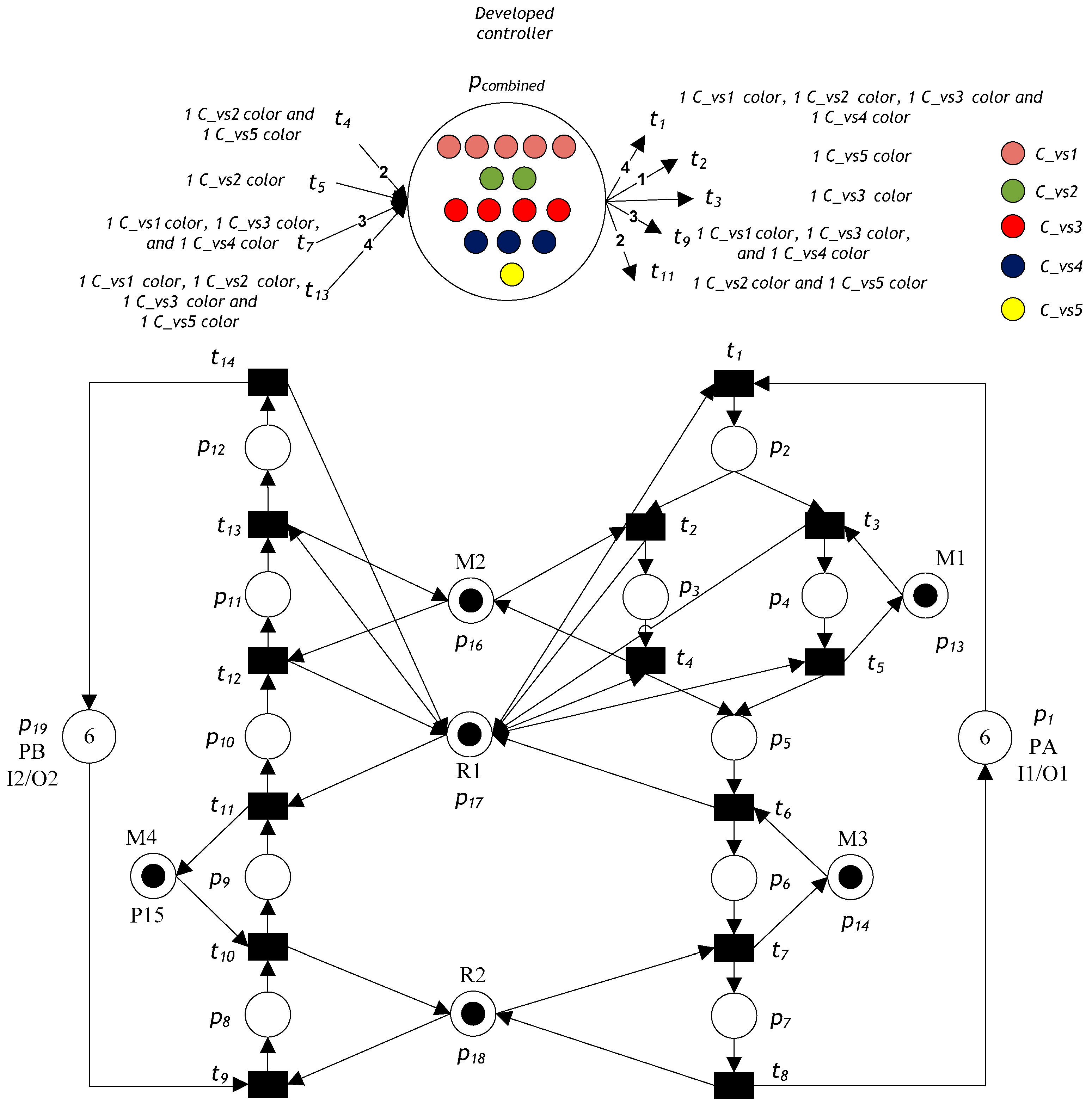
In this section, we show the results of the experiments with the proposed approach. Specifically, we use an AMS example available in the literature: the AMS Petri net model given in Piroddi et al. [30], Chen et al. [8], Chen and Li [31], Chen et al. [32], and TCCPN [26,27,28,29]. The Petri net model is displayed in Figure 11; it includes 14 transitions and 19 places. The places can be described as the following set partition: P⁰ = {p_1, p₁₉}, P_R = {p₁₃, …, p₁₈}, and P_A = {p₂, …, p₁₄}. The properties of the developed Petri net models are obtained using the free GPenSIM tool [22]. We find that it has 282 reachable markings, and the system is not live (it has a deadlock).

We apply the proposed deadlock-prevention algorithm to this case study. Without considering recovery subnets, the system model has five SMSs that may be empty: S₁ = {p₇, p₁₂, p₁₃, p₁₄, p₁₅, p₁₆, p₁₇, p₁₈}, S₂ = {p₅, p₁₂, p₁₃, p₁₆, p₁₇}, S₃ = {p₂, p₇, p₁₂, p₁₄, p₁₅, p₁₆, p₁₇, p₁₈}, S₄ = {p₂, p₇, p₁₀, p₁₂, p₁₄, p₁₅, p₁₇, p₁₈}, and S₅ = {p₂, p₅, p₁₂, p₁₆, p₁₇}. Based on the suggested deadlock-prevention algorithm (Algorithm 1), five monitors are inserted to protect the five SMSs from being emptied. The required control places using Algorithm 1 are designed as follows:

(1)

^•V_S1 = {t₇, t₁₃}, V_S1^• = {t₁, t₉}, and M_Vo(V_S1) = 5.

(2)

^•V_S2 = {t₄, t₅, t₁₃}, V_S2^• = {t₁, t₁₁}, and M_Vo(V_S2) = 2.

(3)

^•V_S3 = {t₇, t₁₃}, V_S3^• = {t₁, t₉}, and M_Vo(V_S3) = 4.

(4)

^•V_S4 = {t₇, t₁₁}, V_S4^• = {t₁, t₉}, and M_Vo(V_S4) = 3.

(5)

^•V_S5 = {t₄, t₁₃}, V_S5^• = {t₂, t₁₁}, and M_Vo(V_S5) = 3.

By Definition 11, a deadlock control subnet of the Petri net model illustrated in Figure 11 is N_DC = (p_combined, {T_DCi, T_DCo}, F_DC, C_vsi), where T_DCo = {4t₁, t₂, t₃, 3t₉, 2t₁₁}, and T_DCi = {2t₄, t₅, 3t₇, 4t₁₃}. The initial token with a color marking of a combined monitor is M_DCo(p_combined) = ∑M_Vo(V_S) = M_Vo(V_S1) + M_Vo(V_S2) + M_Vo(V_S3) + M_Vo(V_S4) + M_Vo(V_S5) = 5 + 2 + 4 + 3 + 1 = 15 tokens. Thus, in the Petri net model illustrated in Figure 11, there are five color types, which are SC = {C_vs1, C_vs2, C_vs3, C_vs4, C_vs5}. Therefore, the total number of colored tokens is 15: five tokens of color C_vs1, two tokens of color C_vs2, four tokens of color C_vs3, three tokens of color C_vs4, and one token of color C_vs5, as shown in Figure 11.

In the net displayed in Figure 11, when transition t₁ fires, the system selects only one token from input place p₁, one token from resource place p_17. Additionally, the system selects tokens from p_combined: one token of color C_vs1, one token of color C_vs2, one token of color C_vs3, and one token of color C_vs4. If transition t₂ is fired, the system selects only one token from place p₂, one token from resource place p₁₆, and one token of color C_vs5 from p_combined. Moreover, when transition t₃ fires, the system selects only one token from input place p₂, one token from resource place p₁₃, and one token of color C_vs3 from p_combined.

If transition t₉ fires, the system selects only one token from input place p₁₉, one token from resource place p₁₈, one token of color C_vs1 from p_combined, one token of color C_vs3 from p_combined, and one token of color C_vs4 from p_combined. In addition, when transition t₁₁ fires, the system selects only one token from input place p₉, one token from resource place p₁₅, one token from resource place p₁₇, one token of color C_vs2 from p_combined, and one token of color C_vs5 from p_combined.

When transition t₄ fires, the system creates two colored tokens—one of color C_vs2 and one of color C_vs5—and transfers them into the common place p_combined. Moreover, when transition t₅ fires, the system adds color C_vs2 to the tokens and transfers them into the common place p_combined. If transition t₇ fires, the system creates three colored tokens—one of color C_vs1, one of color C_vs3, and one of color C_vs4—and transfers them into the common place p_combined. Finally, when transition t₁₃ fires, the system creates four colored tokens—one of color C_vs1, one of color C_vs2, one of color C_vs3, and one of color C_vs5—and transfers them into the common place p_combined.

To test and validate the developed GPenSIM code, we compared it with the methods in Piroddi et al. [30], Chen et al. [8], Chen and Li [31], Chen et al. [32], and TCCPN [26,27,28,29]. The simulation was undertaken for 480 min. After running and simulating the Petri net model in MATLAB, we obtained the results summarized in

Table 2. Comparison with the existing policies: number of monitors, number of arcs, liveness, and reachable marking.

Parameters	Chen et al. [8]	Piroddi et al. [30]	Chen and Li [31]	Chen et al. [32]	TCCPN[26,27,28,29]	Proposed Method
Monitors	8	5	2	2	1	1
Arcs	37	23	12	12	9	9
Liveness	Live	Live	Live	Live	Live	Live
Reachable marking	205	205	205	205	205	205

and

Table 3. Comparison with the existing policies: utilization throughput, work-in-process, and throughput time.

Parameter	Chen et al. [8]	Piroddi et al. [30]	Chen and Li [31]	Chen et al. [32]	TCCPN [26,27,28,29]	Proposed Method
M 1 utilization%	18.75	17.7083	17.7083	17.7083	17.7083	17.7083
M 2 utilization%	35	33.3333	33.3333	33.3333	34.5833	33.9583
M 3 utilization%	12.5	13.75	14.375	14.375	11.875	12.5
M 4 utilization%	22.5	21.6667	20.8333	20.8333	23.3333	22.5
R 1 utilization%	39.5833	40	40.4167	40.4167	39.1666	39.58333
R 2 utilization%	29.375	30	30	30	30	30
Throughput of Part A (unit)	20	21	20	20	19	24
Throughput of Part B (unit)	26	25	26	26	27	23
Work-In-Process	3.9271	3.93331	3.8480	3.9667	3.4938	3.3854
Throughput time of Part A (min)	23.9500	22.8571	24	23.9235	25.2105	19.9583
Throughput time of Part B (min)	18.4230	19.200	18.3321	18.4615	17.7407	20.8260

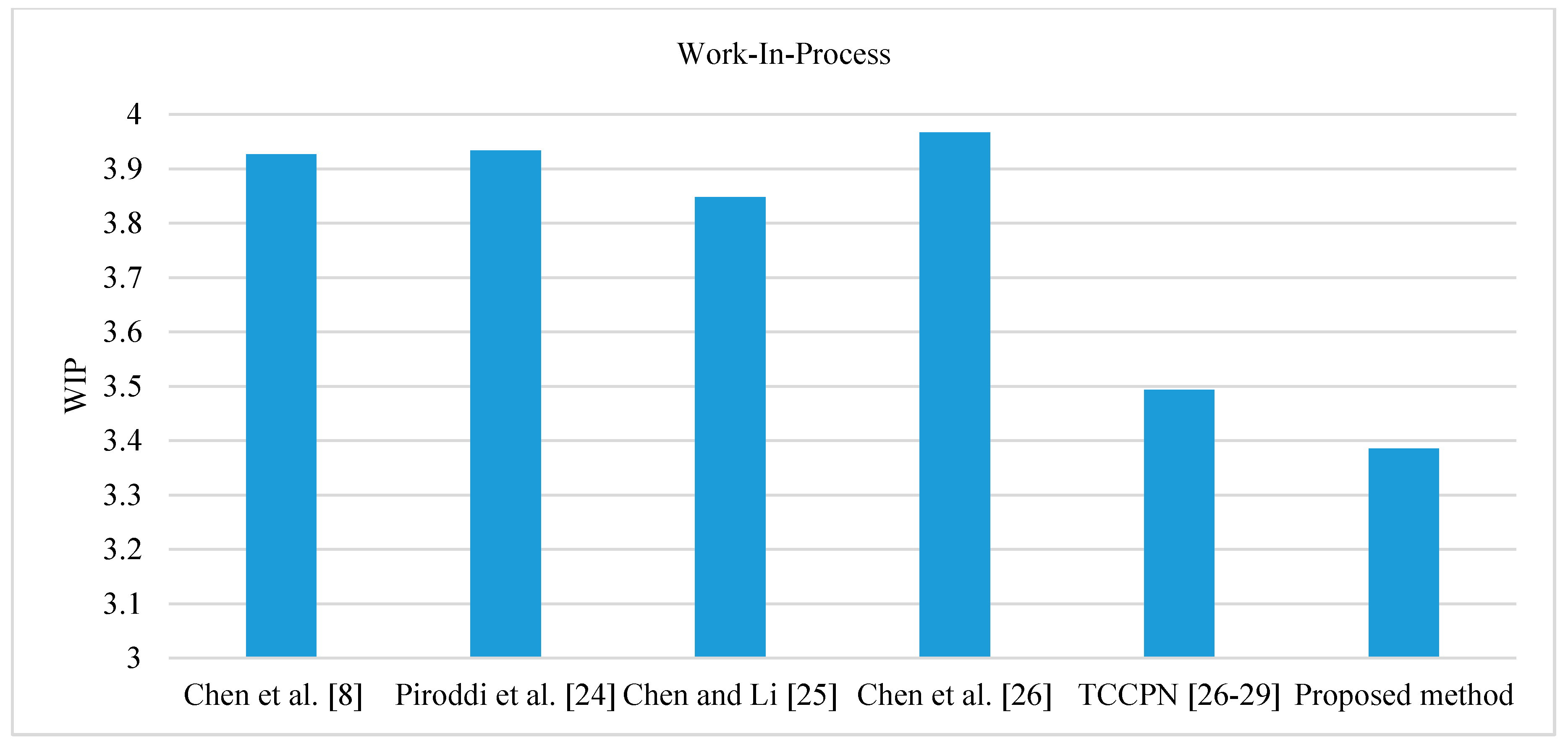
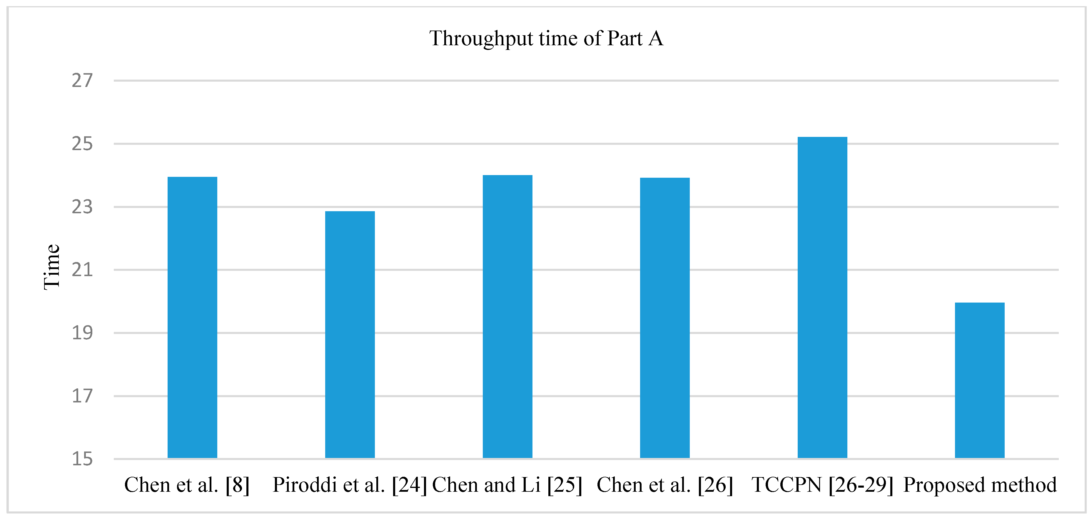
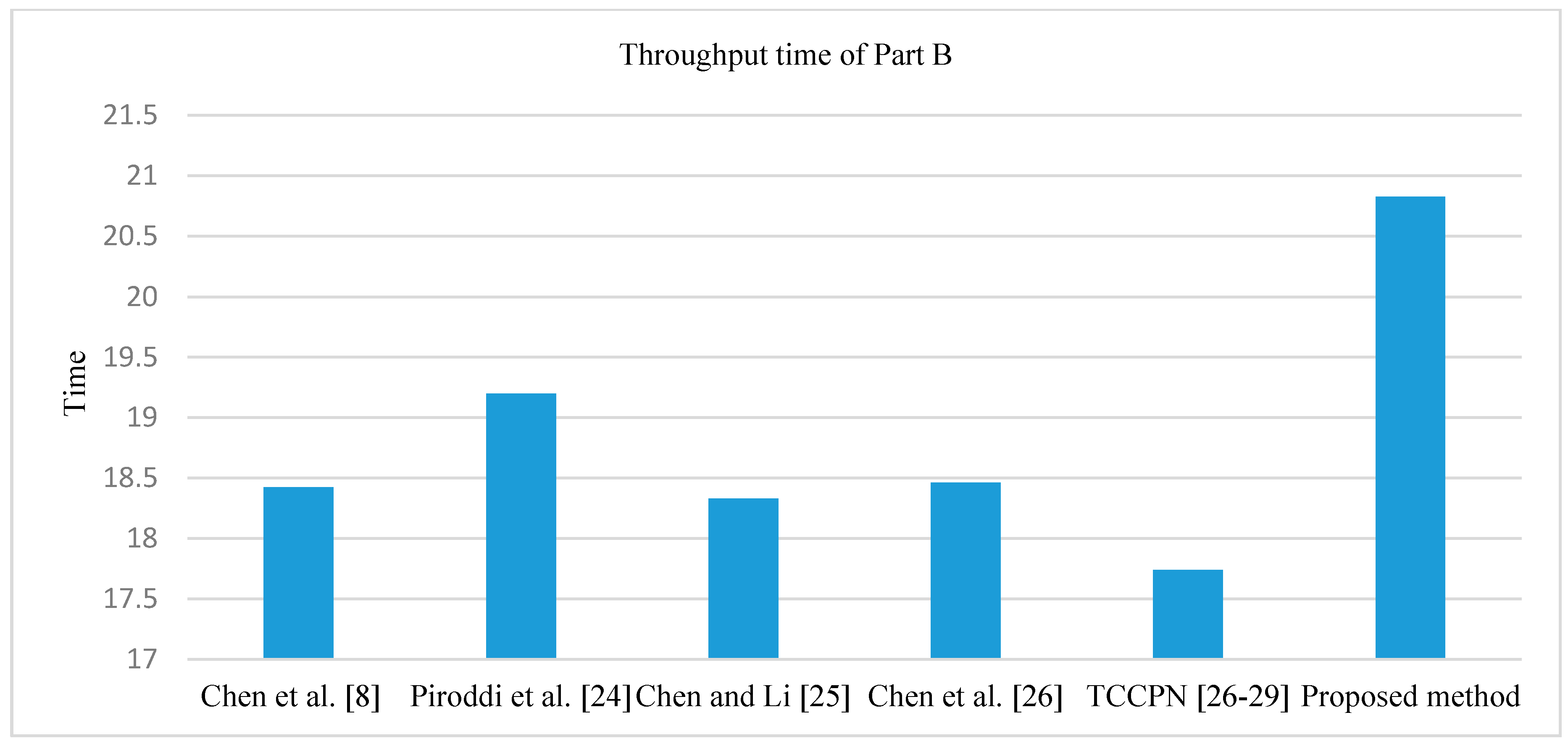
. Table 2 shows the results in terms of the number of monitors, number of arcs, liveness, and reachable marking. We observe that the proposed approach provides a supervisor with only a single control place and 9 arcs, both of which are minimal compared with other techniques in Piroddi et al. [30], Chen et al. [8], Chen and Li [31], and Chen et al. [32]. Table 3 displays the results in terms of utilization of the robots and machines, throughput of Part A and Part B, work-in-process (WIP), and total time in system (throughput time). In terms of the resource utilization, all methods obtain approximately the same values, as shown in Figure 12. Moreover, from the viewpoint throughput, the proposed method can provide greater throughput than other techniques as shown in Figure 13. In term of WIP, the proposed method leads to better WIP than the other techniques as shown in Figure 14. With respect to throughput time of Part A and Part B, overall, the proposed method can obtain less throughput time than other techniques as shown in Figure 15 and Figure 16. Therefore, the proposed method is valid, it can give sufficiently accurate results, and it can potentially be applied to other cases.

5. Conclusions

In this paper, we introduce a two-step controlled deadlock policy. In the first step, we create a Petri net controlled model using the deadlock prevention method based on SMSs proposed by [1]. In the second step, all control places obtained after the first step are merged into a single control place based on the colored Petri nets to mark all SMSs. We compare the proposed method with the methods of Piroddi et al. [30], Chen et al. [8], Chen and Li [31], and Chen et al. [32], and TCCPN [26,27,28,29]. According to our results, the proposed controller is more powerful, has a simpler structure, and does not need to calculate reachability graphs; therefore, it has low-overhead computation. The most challenging research topic in the future is that the controlled system that developed by previous deadlock control approaches may undergo changes of control requirements and specifications such as:

• Adding or removing a machine
• New production ratio
• Adding new product
• Changing a resource capacity
• Resource faults and raw-material processing in a faulty resource
• The processing routes of the system are changed
• System contain uncontrollable transitions

When a system has these problems, a system needs to be reconfigurable. Then the deadlock-free system can have deadlocks. Therefore, the proposed robust deadlock control policy needs to be extended to improve efficiency for rapid and valid reconfiguration of Petri net-based supervisory controllers for reconfigurable manufacturing systems.