A Comparison of Clustering and Prediction Methods for Identifying Key Chemical–Biological Features Affecting Bioreactor Performance

Abstract

Chemical–biological systems, such as bioreactors, contain stochastic and non-linear interactions which are difficult to characterize. The highly complex interactions between microbial species and communities may not be sufficiently captured using first-principles, stationary, or low-dimensional models. This paper compares and contrasts multiple data analysis strategies, which include three predictive models (random forests, support vector machines, and neural networks), three clustering models (hierarchical, Gaussian mixtures, and Dirichlet mixtures), and two feature selection approaches (mean decrease in accuracy and its conditional variant). These methods not only predict the bioreactor outcome with sufficient accuracy, but the important features correlated with said outcome are also identified. The novelty of this work lies in the extensive exploration and critique of a wide arsenal of methods instead of single methods, as observed in many papers of similar nature. The results show that random forest models predict the test set outcomes with the highest accuracy. The identified contributory features include process features which agree with domain knowledge, as well as several different biomarker operational taxonomic units (OTUs). The results reinforce the notion that both chemical and biological features significantly affect bioreactor performance. However, they also indicate that the quality of the biological features can be improved by considering non-clustering methods, which may better represent the true behaviour within the OTU communities.

1. Introduction

Process analytics in the chemical and biotechnology industries is currently reaping the rewards from a data revolution, which was initiated in the 1980s in the field of computer science and communications. This sparked the development of machine learning (ML) modeling paradigms. Simpler models such as random forests [1] and support vector machines [2] have demonstrated widespread success in a variety of classification problems; some examples include invasive plant species prediction [3] and speech recognition [4]. The highly complex neural networks [5] have been recognized as universal approximators [6] for non-linear functions. Neural networks are being successfully applied to modern problems such as natural language processing [7], image prediction [8], and recommender systems [9]. The success of neural nets lie in their ability to handle datasets with exorbitant numbers of samples (e.g., billions), which are known as big-N problems.

On the other hand, data are relatively scarce in the field of process engineering. For example, concentrations of chemicals or populations of biological specimens are usually measured intermittently in laboratories; this limits the frequency at which these data can be acquired. Currently there are few online, ML-based soft sensors for these measurements that are both accurate and inexpensive. Due to both the economical and physical limitations of obtaining abundant data in these cases, biological systems are usually known as small-N problems. In addition to being small-N, these datasets are often also high-dimensionality or big-d. The high number of features in these cases render many simple ML algorithms infeasible, due to the curse of dimensionality [10]. In light of these marked distinctions, these problems warrant an entirely different modeling and analysis paradigm. This study will address some of these challenges, by providing a sensible analysis workflow that identifies key features correlated with a predicted outcome.

The challenges of analyzing chemical, biological, and process data are non-trivial. Interpretable patterns—such as correlations between process performance and features—are often confounded due to the following inexhaustible list of factors:

• Non-uniform and inconsistent sampling intervals.
• Order-of-magnitude differences in dimensionalities.
• Complex interactions between participating species in a bioreactor (e.g., protagonistic vs. antagonistic members, functionally-redundant members).
• Conditionally-dependent effects of features (i.e., some features only affect the outcome in the presence or absence of other features).

Biological system data often includes the relative abundances of operational taxonomic units (OTUs). An OTU represents a taxonomic group (e.g., species or genus) based on the similarity (e.g., $97\%$ or $95\%$ for species and genus, respectively) of their 16S rRNA variable regions. These are determined using high-throughput sequencing of microbial community DNA [11]. The environment inside a bioreactor contains chemical and physical factors, which influence the types of OTUs that thrive. Conversely, the OTUs themselves also affect the environmental conditions inside the bioreactor, since microorganisms mediate many different types of chemical reactions. Microorganisms are known to interact and form communities with members that are protagonistic, antagonistic, or simply bystanders [12]. These profound coupling effects are difficult to identify as closed-form expressions, due to the non-linear stochastic nature of OTU communities. The individual and group effects of members comprising of thousands of OTUs are extremely difficult to isolate. However, the overall confusion can be significantly alleviated by first grouping or clustering OTUs together, according to pre-specified similarity metrics [13]. This reduces the dimensionality of analysis exponentially (e.g., from a few hundred down to several features), which in turn allows the predictive models to be much more focused. Grouping or clustering of OTUs is done with the purpose of identifying so-called keystone microorganisms, or biomarkers, which correlate to successful versus poor process performance.

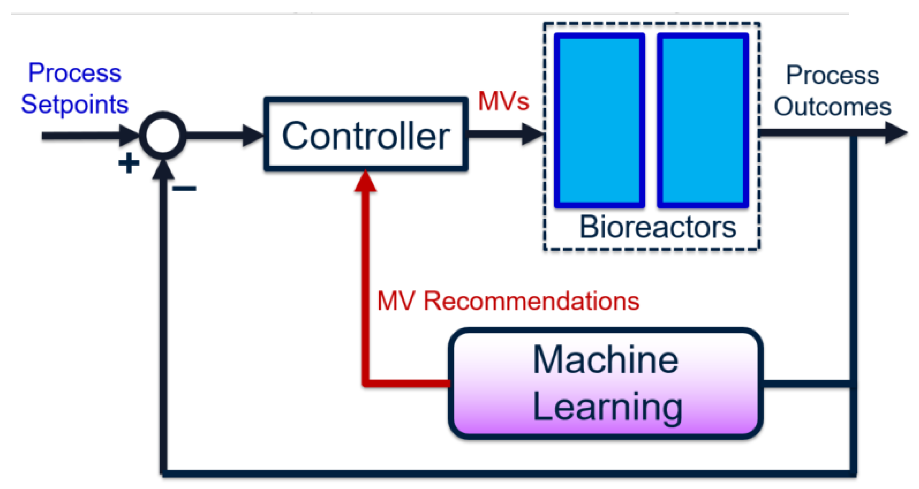
The overall goal for bioreactor modeling is to extract, out of the many chemical, biological, and process features, those that have a proportionally significant effect on process performance. These can be incorporated into a process control algorithm (e.g., involving soft sensors) to improve performance and reliability, by using easy-to-measure features or biomarkers. Given historical data, the process outcome is identified and preferably separated into discrete classes. The high feature-space of the raw data associated with these classes are “compressed” using dimensionality-reduction techniques. This produces smaller subsets of meaningful, representative features. Predictive models are built using these high-impact features, instead of the original feature set (which may contain irrelevant or redundant data). Finally, the representative features are ranked in terms of importance—with respect to their contributions to the final process outcomes—using univariate feature selection techniques. The results from this approach serve as an informative pre-cursor to decision-making and control, especially in processes where little to no prior domain knowledge is available. The entire framework can also be depicted as a closed-loop feedback control diagram [14], as shown in Figure 1.

In the proposed workflow, the choice of manipulated variables (MVs) is dynamic—it is re-identified given each influx of new data. On the other hand, traditional feedback control uses a static set of pre-specified MVs, which may not always be impactful variables if the process and/or noise dynamics vary with time. Specifically, the use of machine learning achieves a three-fold goal:

• During each operating stage, operators would only need to monitor a small set of variables, instead of hundreds or thousands. This simplifies the controller tuning and maintenance drastically, and undesirable multivariable effects (such as input coupling [14]) are reduced.
• By using data-based ML models, the process outcomes can be predicted ahead of time, such that unsatisfactory outcomes are prevented. Moreover, the models can be updated using new data collected from each new operating stage, eliminating the need for complete re-identification.
• The ranking of feature impacts can be performed using grey-box models, which are mostly empirical but are guided by a modest amount of system domain knowledge. This combination is exceptionally powerful if the domain knowledge is accurate, since it defines otherwise-unknown prior assumptions. This improves both prediction accuracy and feature analysis accuracy. The task of control and monitoring is also much more feasible, since the focus is only on a handful of variables (as opposed to hundreds).

This work represents a framework of the feature extraction workflow that precedes the development of the aforementioned process control philosophy. Within the framework, we test several popular techniques for dimensionality reduction and machine learning. The explored techniques are applied on a biological wastewater treatment process aimed at removing selenium. The first part of this paper outlines a systematic data pre-processing workflow, which combines both chemical and biological data in a way that ensures both exert equal weights on the model outcome. Then, three unsupervised learning techniques, hierarchical clustering, Gaussian mixtures, and Dirichlet mixtures, are used dimensionality-reduction techniques to extract biomarkers. These key features, along with water chemistry features, are passed as inputs into three state-of-the-art predictive models to predict the final process outcome of selenium removal rate. The supervised learning techniques used are random forests (RFs), support vector machines (SVMs), and artificial neural networks (ANNs). Finally, important process features are correlated with the selenium removal rate using two techniques: mean decrease in accuracy (MDA), and the conditionally-permutated variant, C-MDA. The quality of modeling and feature selection results are compared and contrasted across all explored methods.

One key difference between this work and others in the literature is the broad range of exploration, as well as the extensive use of compare and contrast for several methodologies of data analysis. Most papers focus on the proof-of-concept and results of a single technique, with focus on either the prediction task or feature analysis task. When reading this paper, the reader should focus more on the strengths and limitations of each method, given the results obtained, rather than the numerical values of the results themselves. The main goal of this work is to bring clarity to the appropriate use of analytics, given the various characteristics and circumstances of the available raw process data.

2. Methods

This section introduces the details behind the wastewater treatment process, as well as the machine learning algorithms used for dimensionality reduction, prediction, then finally feature selection.

2.1. Process Flow Diagram and Description

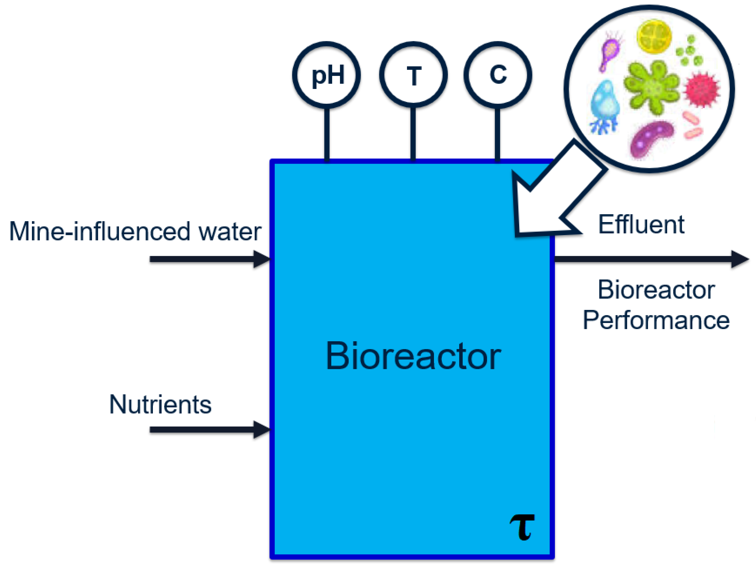
The relevant case study is a wastewater treatment process located downstream of a mining operation. Due to proprietary reasons, the descriptions provided are kept at a general level. The overall process can be visualized as the general bioreactor shown in Figure 2:

Selenate and nitrate concentrations in the bioreactor effluent must be reduced to below $10\frac{\mathsf{\mu }\mathrm{g}}{\mathrm{L}}$ and $3\frac{\mathrm{mg}}{\mathrm{L}}$, respectively [15,16]. These chemical species bio-accumulate in the marine ecosystem [17] and thus reach harmful levels at the top of the food chain.

The feed to the first reactor is wastewater, which contains the main pollutant selenate (SeO${}_4^{2-}$). The selenate is to be reduced to elemental selenium (Se) by a series of two bioreactors. Samples are extracted from the bioreactors during each operating stage (at irregular intervals) and analyzed in order to determine and record values of various water chemistry variables. These features are summarized in

Table 1. Water chemistry variables.

Variable	Description
$\tau$ or EBCT	Empty bed contact time $=\frac{\mathrm{volume}}{\mathrm{flowrate}}$ (min)
$Ammoni{a}_{out}$	Concentration of $N{H}_3$ in effluent $\left(\frac{\mathrm{mg}}{\mathrm{L}}\right)$
$Nitrat{e}_{in}$	Concentration of $N{O}_3^{-}$ in influent $\left(\frac{\mathrm{mg}}{\mathrm{L}}\right)$
$Nitrit{e}_{out}$	Concentration of $N{O}_2^{-}$ in effluent $\left(\frac{\mathrm{mg}}{\mathrm{L}}\right)$
$Se{D}_{in}$	Concentration of total dissolved $Se$ in influent $\left(\frac{\mathsf{\mu }\mathrm{g}}{\mathrm{L}}\right)$
$CO{D}_{in}$	Chemical oxygen demand in the influent $\left(\frac{\mathrm{mg}}{\mathrm{L}}\right)$
$MicroC$	Equal to 1 if MicroC is added as carbon source, otherwise 0
$Acetate$	Equal to 1 if Acetate is added as carbon source, otherwise 0
Reactor 1	Equal to 1 if Reactor 1 is the relevant bioreactor, otherwise 0
Reactor 2	Equal to 1 if Reactor 2 is the relevant bioreactor, otherwise 0

.

In addition to the water chemistry data, data pertaining to the microbial presence is available in the form of operational taxonomic units (OTUs). In this case study, the numerical values associated with each OTU are known as raw abundance counts. These counts can be considered normalized population counts of each bacterial species, which fall within the range of 0∼16,000.

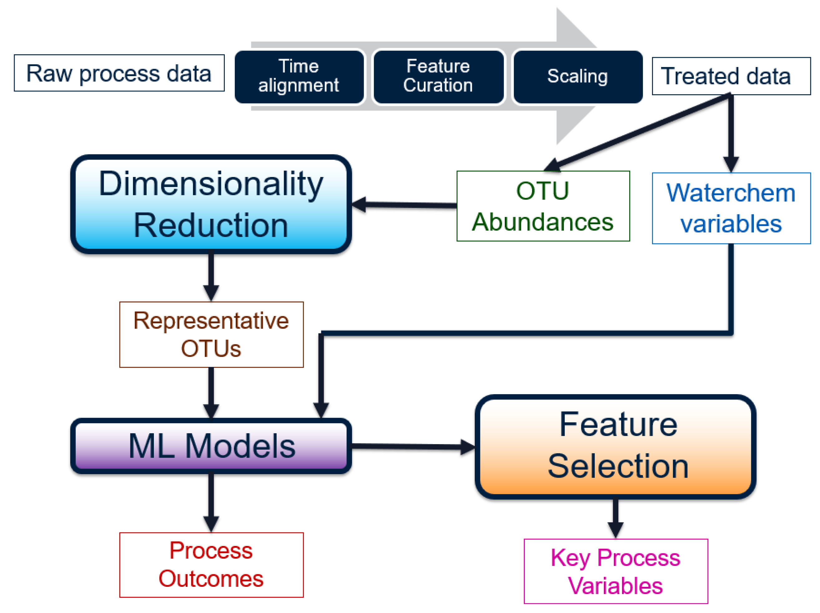
2.2. Data Pre-Treatment

Before the raw water chemistry and micro-biological data can be used for any analysis, they must be transformed into a meaningful form. The steps involved can be visualized as a workflow in Figure 3.

The data pre-processing was performed using Jupyter iPython notebooks. The raw dataset originally consists of two files: one containing water chemistry data, and one containing OTU counts. First, samples containing missing or $NaN$ values were removed using the dropna function in pandas. Then, spurious process values (such as negative flowrates) were removed by Boolean functions. The remaining samples were then cross-matched between the water chemistry and OTU files, by use of $SampleID$ tags which identify common operating stages. This results in a total of $N=56$ samples containing both water chemistry and microbial information. Although this is a small sample-size, it is unfortunately all the data that could be collected from this treatment plant.

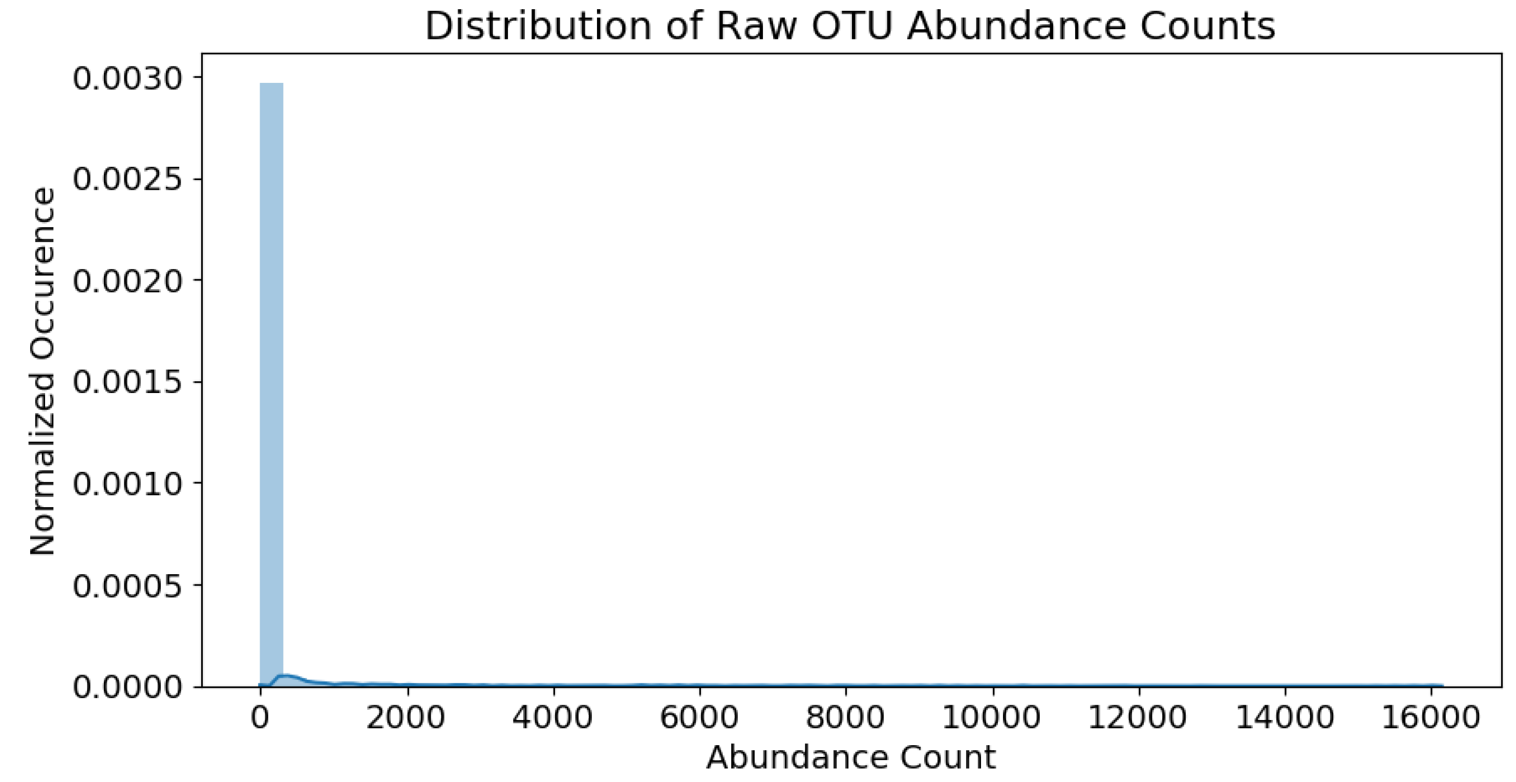
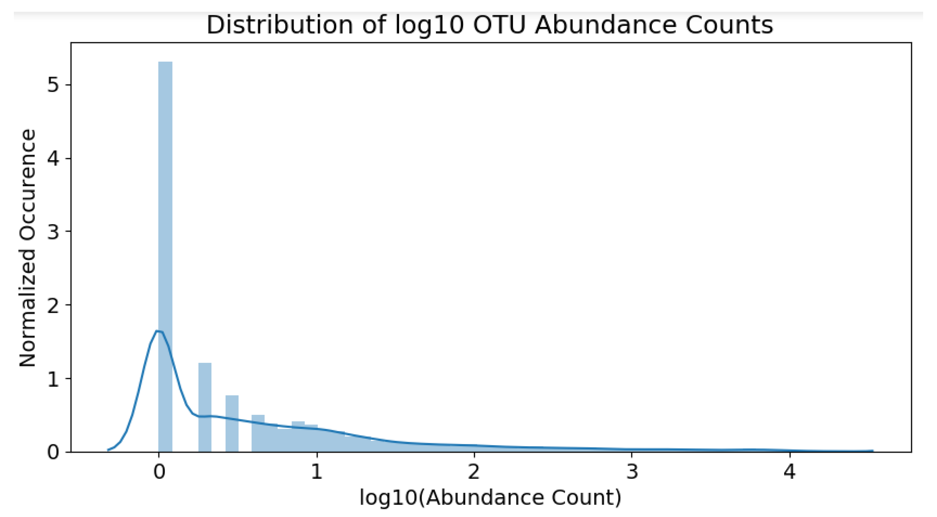
Each water chemistry variable outlined in Table 1 (except SampleID) is standardized via mean-centering and unit-variance operations. This removes any weight-skewing effects during modeling, due to varying feature ranges. The OTU raw abundance counts are recorded in a matrix where the number of samples and number of OTUs are $N=56$ and $d_{OTU}=305$, respectively. The raw counts fall within the range of 0∼16,000. The abundance distribution is heavily skewed towards the lower population numbers, as shown in Figure 4.

The skew is partially remedied by applying a $lo{g}_{10}$-transformation to all raw counts. Since many raw counts are equal to zero, 1 is added to every value before the $lo{g}_{10}$ transformation, to ensure the $lo{g}_{10}$ operation is valid. Counts equal to zero would still remain zero after transformation, since $lo{g}_{10}(0+1)=0$. The overall operation is:

$$\begin{array}{c}\hfill {\mathrm{Count}}_{\mathrm{scaled}}=lo{g}_{10}({\mathrm{Count}}_{\mathrm{raw}}+1)\end{array}$$

(1)

The resulting distribution of the scaled counts can be observed in Figure 5. Note that the skew is not as severe as before; the OTU population distribution is now much clearer.

These counts are now in a suitable form for analysis methods outlined in the following sections.

2.3. Unsupervised Learning Methods

The goal of unsupervised data analysis is to delve within the existing data, to search for patterns (e.g., clusters or latent variables) that serve as indicators responsible for the observed outcomes. Although some popular algorithms such k-Means [18] or density-based clustering [19] come to mind, they are not suitable for this case study. This is due to the relatively poorer performance of these methods in high-dimensional datasets, a phenomenon known as the curse of dimensionality.

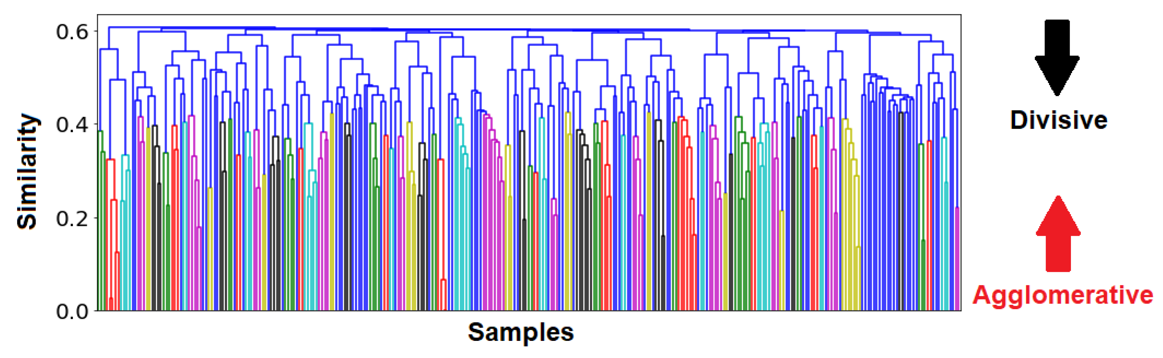
Instead, this work will primarily focus on three clustering algorithms. The first is known as hierarchical clustering [20,21], which groups organisms together according to a similarity metric. The sizes of the groups can be arbitrarily selected, by deciding the position on the ranking system of said organisms. The benefit of this method lies in the ability to visualize not only the individual groups, but also the relationship between various groups on a dendrogram (see Figure A6), as well as their comparative sizes. Pertinent details behind this technique can be found in Appendix H.

The second and third clustering methods are probabilistic mixtures: namely, the Gaussian [22] and Dirichlet multinomial mixtures [23,24]. These mixture models are used to cluster OTUs based on assumptions of their underlying distributions, rather than their pairwise similarities. The optimal clusters are identified by using the well-known expectation–maximization (EM) algorithm [25]. The remaining details behind these mixtures can be found in Appendix I.

2.4. Network Analysis

Network analysis is a pre-processing technique used in this work, which transforms raw data (such as OTU abundance counts) into association values. These associations can be considered a statistical verification of co-occurrence between OTUs, which estimates true partial correlations between pairwise species.

The basis for this method comes from the observation that communities of microorganisms are extremely complex, and exert confounding effects on process outcomes. For example, OTU communities consist of members which are protagonistic, antagonistic, bystanding, and functionally- redundant species. Although the predatory-prey Lotka-Volterra model [26,27] is a popular method of clarifying such relationships, the network analysis and networks to models strategies [28] are a more modern and relevant approach to the case study at hand. The results from [29] show that not only can dominant microbial groups be directly linked to a certain outcome, but indirect species which faciliate these interactions can also be identified. These network associations can be readily computed using the netassoc algorithm [30]. In summary, this algorithm models the indirect effects of a possible third species (or more) that affects the primary interaction between the main two pairwise species, which is akin to conditionally-dependent modeling in Bayesian networks [31]. The main advantage of this approach is the ability to identify both biomarkers and secondary OTUs, which either facilitate or inhibit a specified process outcome (e.g., removal rate).

2.5. Supervised Learning Methods

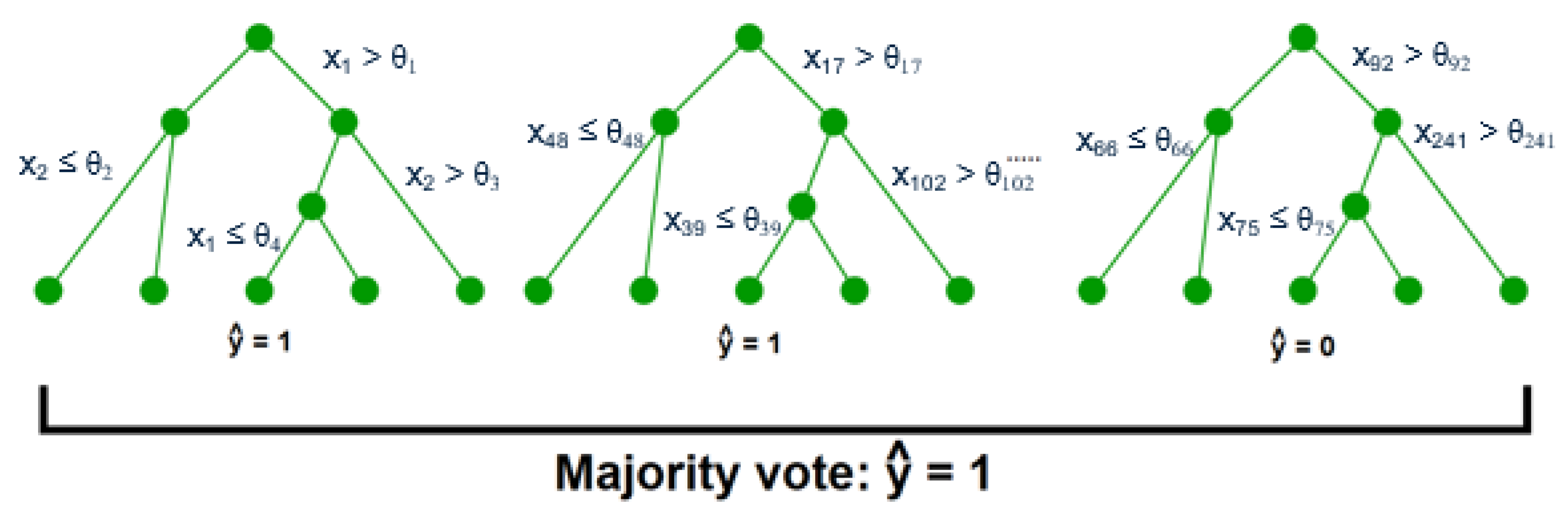
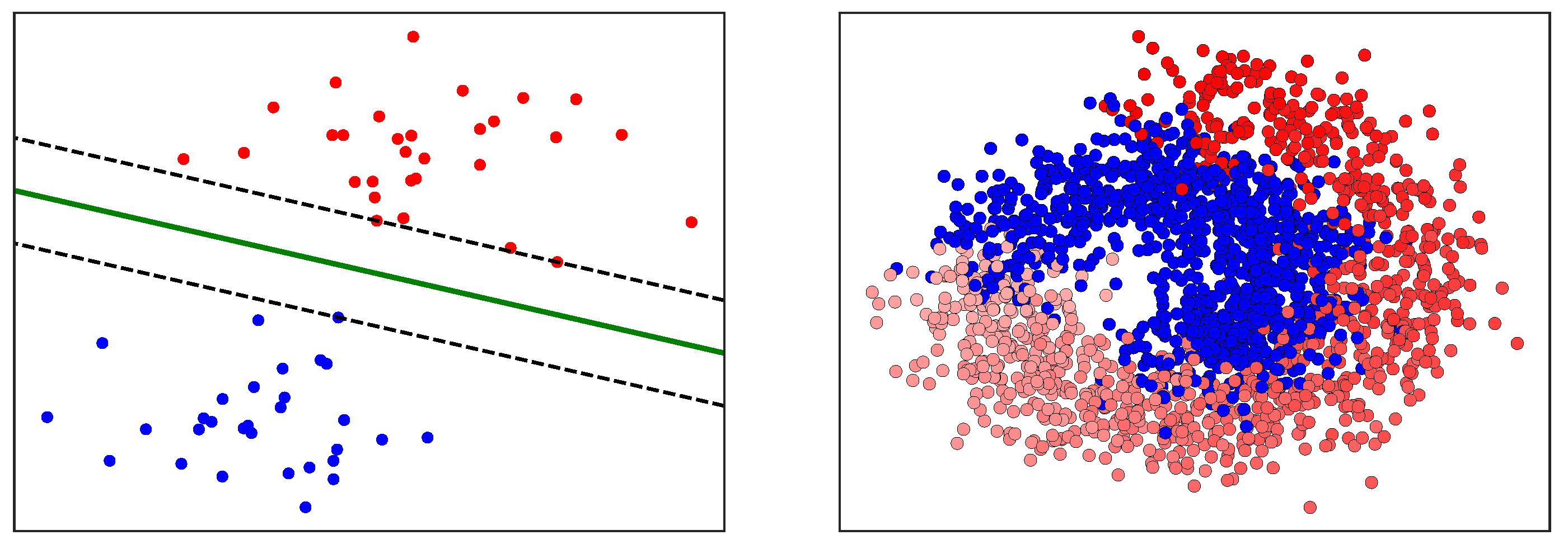
After the key variables have been identified using the previous dimensionality reduction and network analysis methods, they are used to perform predictions of the final process outcome. Prediction plays a vital role in process control; if the variable(s) of interest are estimated before actual occurrence, then remedial actions can be formulated ahead of time. In this case study, the primary process outcome of selenium removal rate is predicted using three supervised learning techniques. 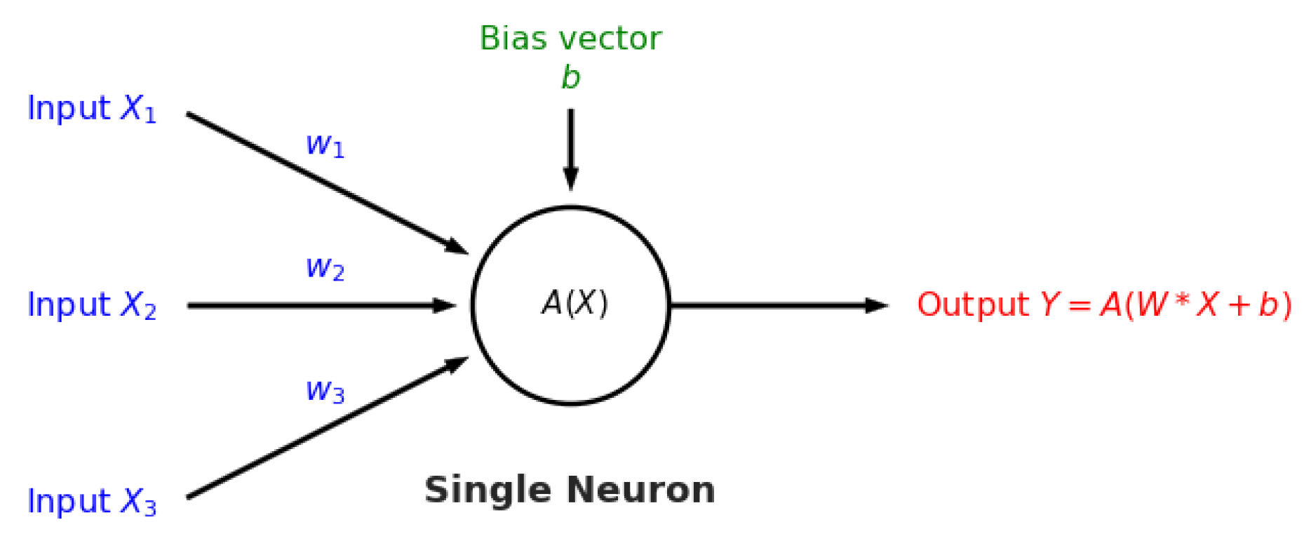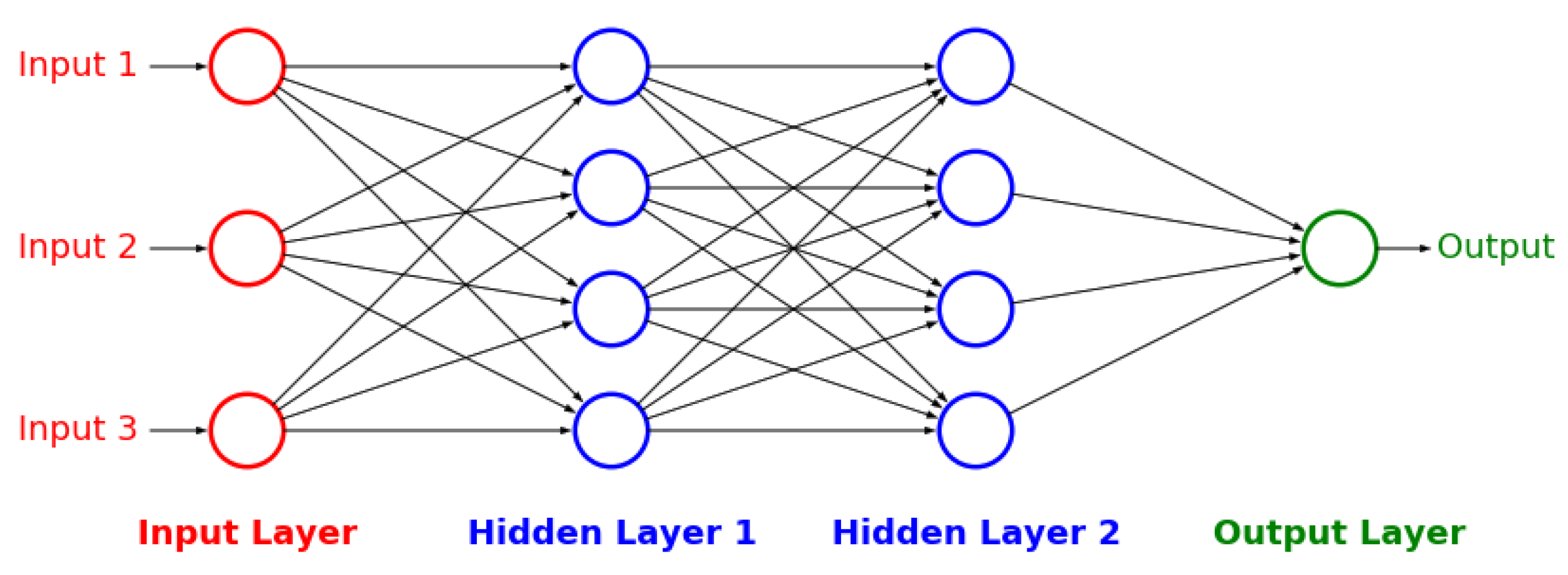These include random forests [1], support vector machines [2] (Figure A3), and artificial neural networks [32] (Figure A4 and Figure A5). The details behind these well-known models can be found in Appendix E, Appendix F and Appendix G respectively.

2.6. Feature Selection

After the key features have been identified and used to predict the final process outcome, a natural question to ask from a process engineering perspective is: “Which of these features contribute the most to the predictions?” Although most feature selection approaches in literature are often selected and customized on a case-by-case basis, two overarching groups of methods can be identified:

• Hypothesis testing: A model is trained with all features left untouched. Then, features are either removed or permutated (scrambled), either individually or conditionally according to other features. The model is re-trained, and its accuracy is compared to the base-case accuracy. The features which cause the largest decreases in model accuracy are considered “most important,” and vice versa.
• Scoring: A metric or “score” based on information or cross-entropy is defined and calculated for all features. Features with the highest scores are identified as the “most relevant,” and vice versa.

In the hypothesis testing framework, univariate (or single-feature) algorithms such as mean decrease in accuracy (MDA), and mean Gini impurity (MGI) [33] have been developed for simple models such as random forests. The MDA method can be visualized in Figure 6.

Unfortunately, these univariate approaches have the following shortcomings:

• Inability to recognize coupling effects between multiple features, such as correlations or redundancies [34].
• Inability to distinguish conditional effects between features, i.e., whether a feature is “relevant” given the presence of other feature(s).

The second point above confounds the definition of “relevance.” A classic example is the prediction of presence of genetic disease (the outcome) using the genetic information of a person’s mother and grandmother. If information from the mother is absent, then the grandmother’s genes may be identified as a “relevant” feature. However, if genetic information is present from both the mother and grandmother, then the grandmother’s genes may become “redundant” and thus an “irrelevant” feature. Therefore, the “relevance” of a feature can be contingent or conditional on the presence of other features. 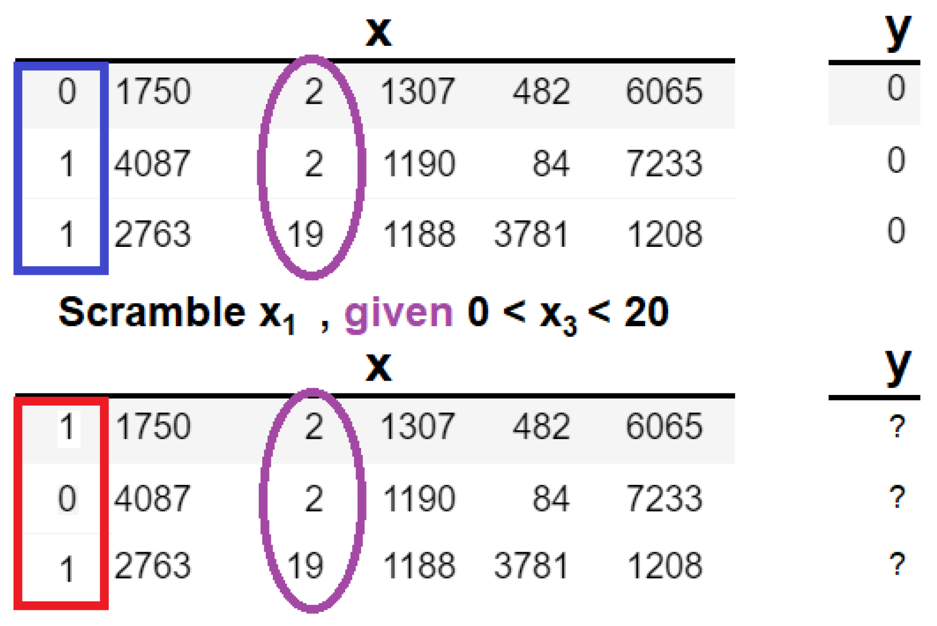The authors in [35] have made significant contributions to the modeling of conditional dependencies. The authors proposed an approach known as conditional mean decrease in accuracy (C-MDA), which is a variation on classic MDA, where conditional permutations are performed given the presence of other features. The conditional is defined as the appearance of secondary features within specified ranges of values. The difference in permutation between MDA and C-MDA can be realized in Figure 7.

3. Results

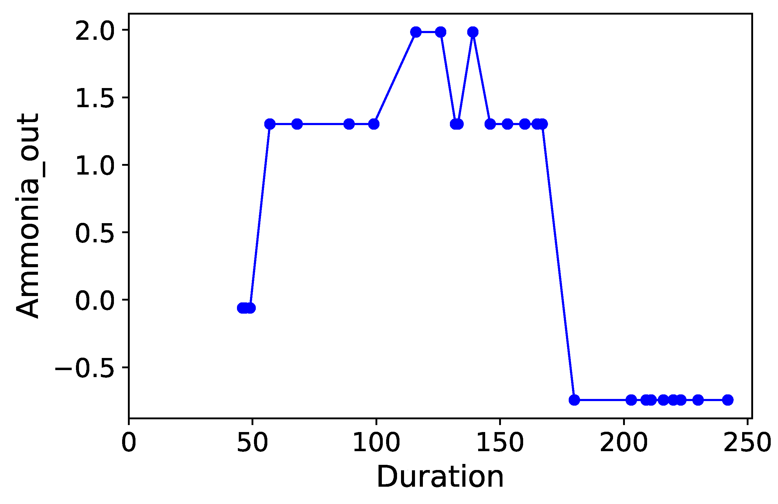
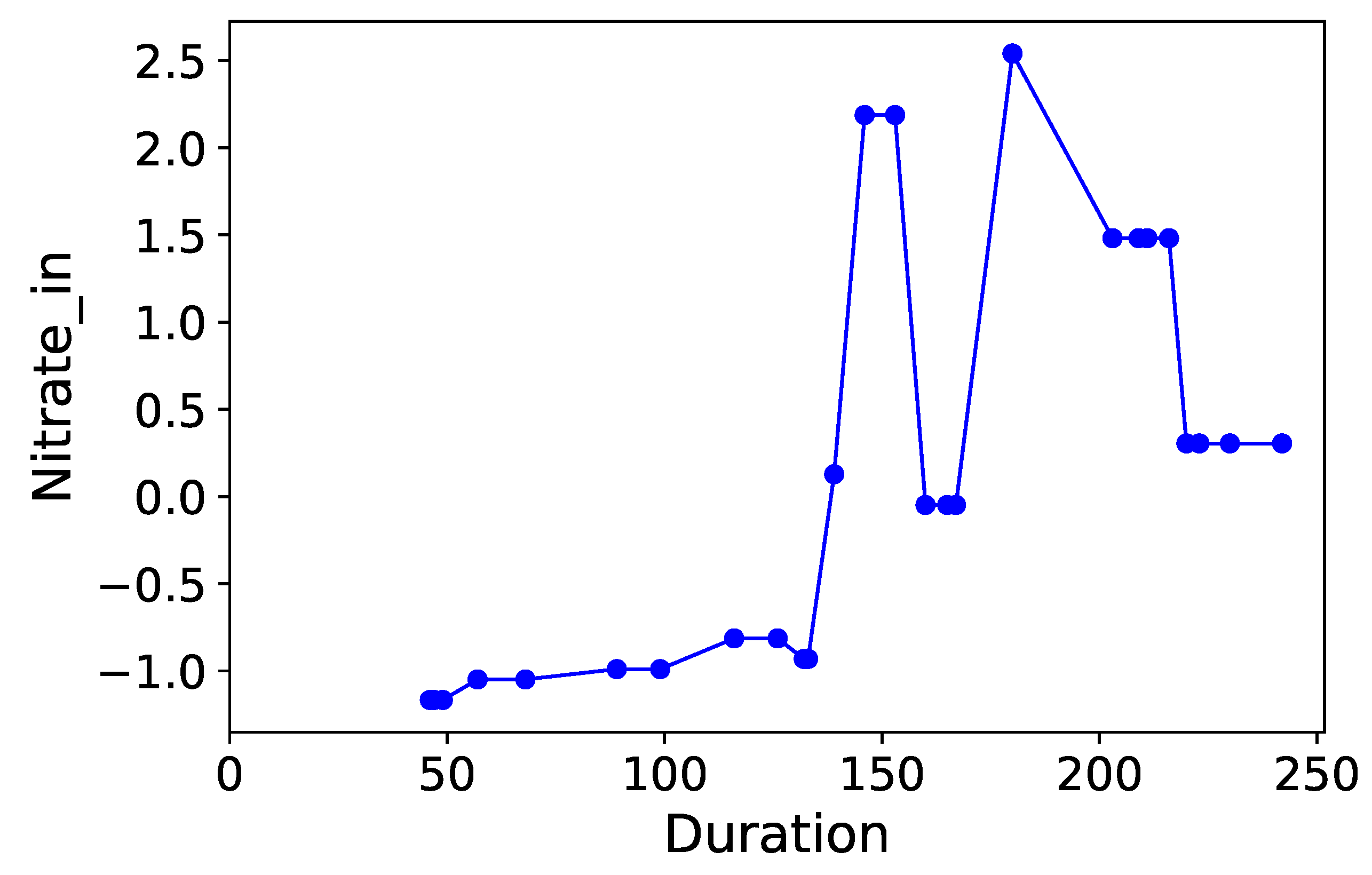
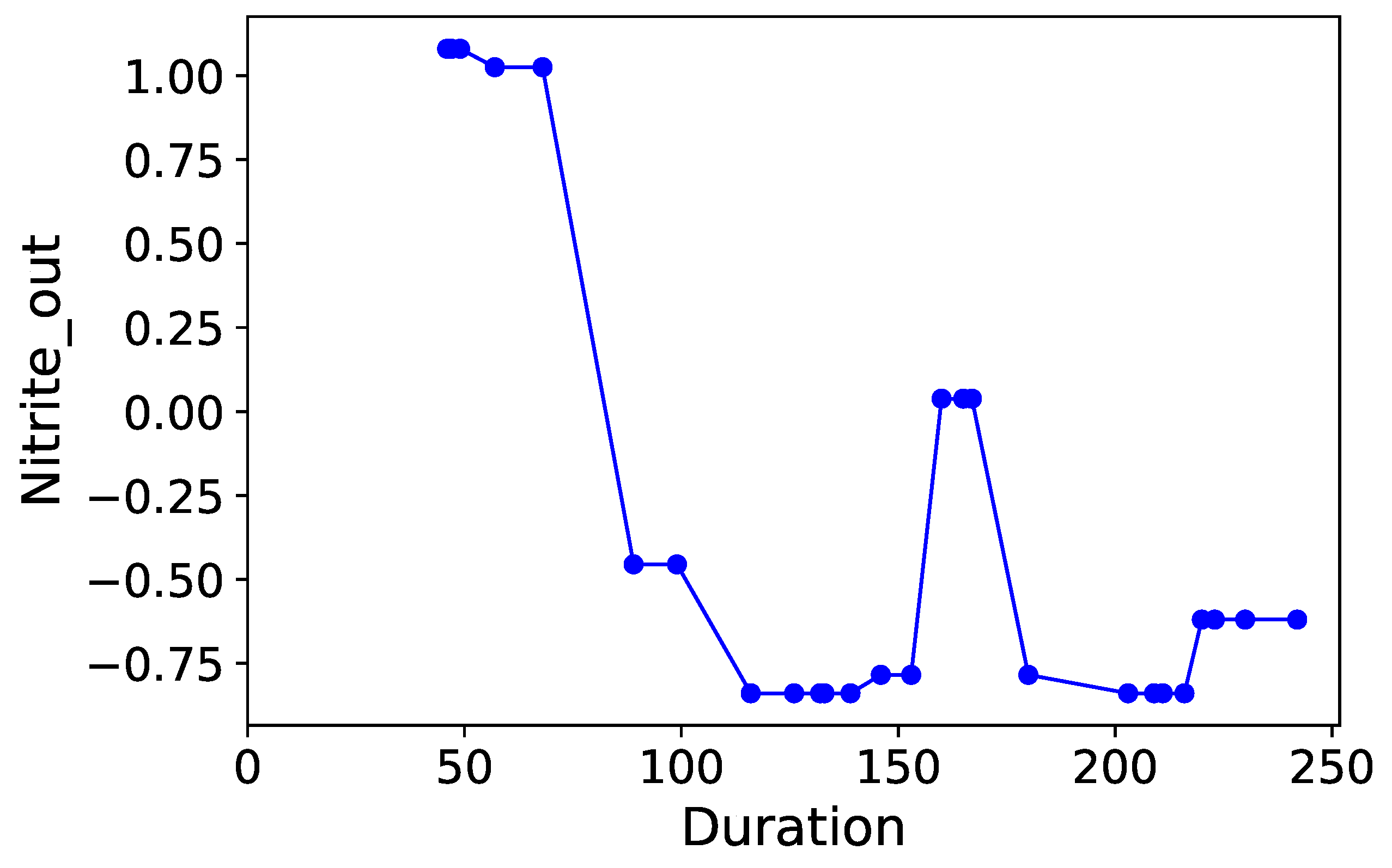
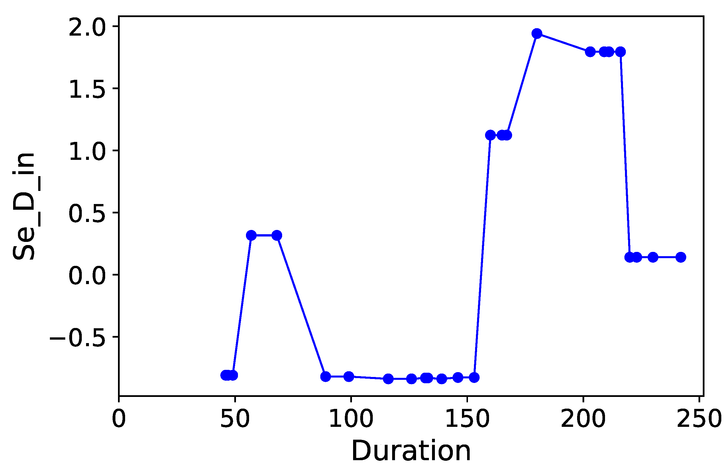
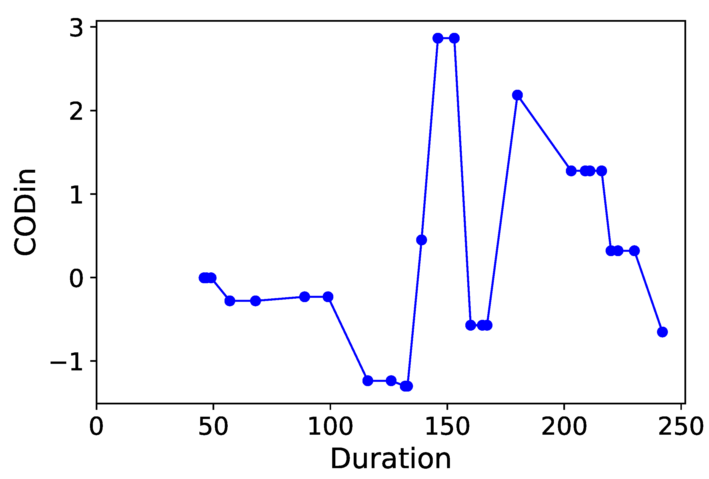
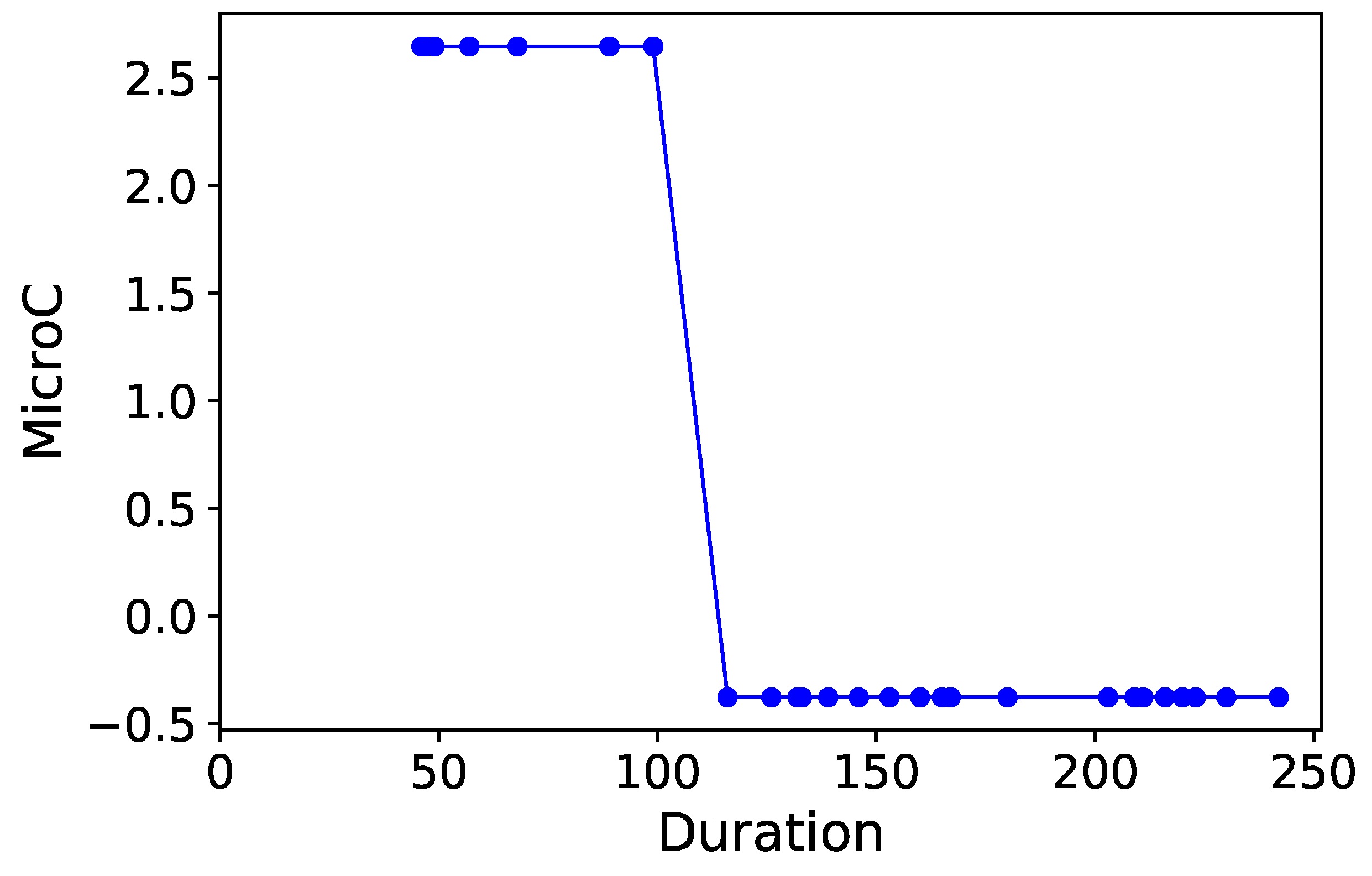
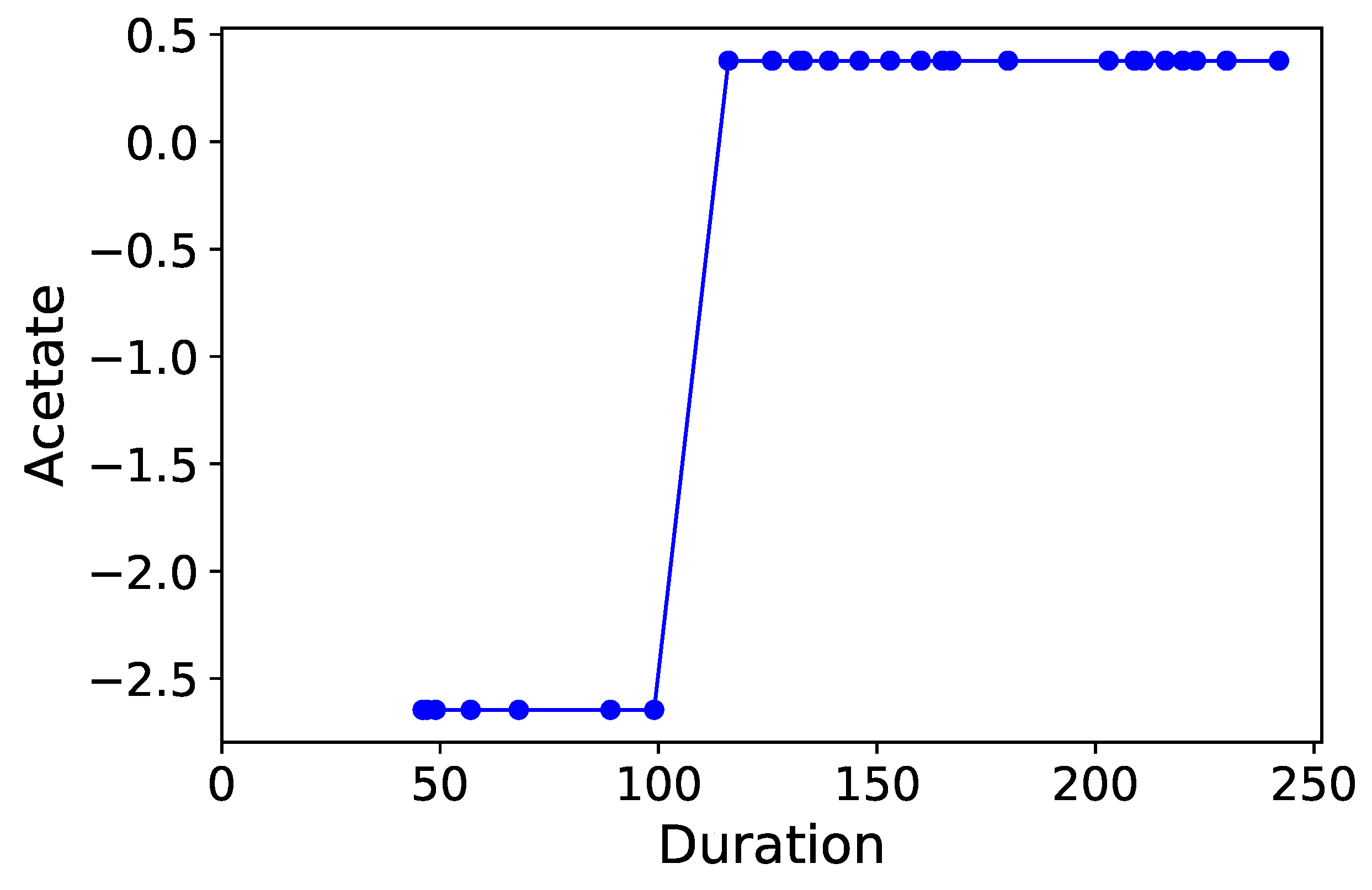
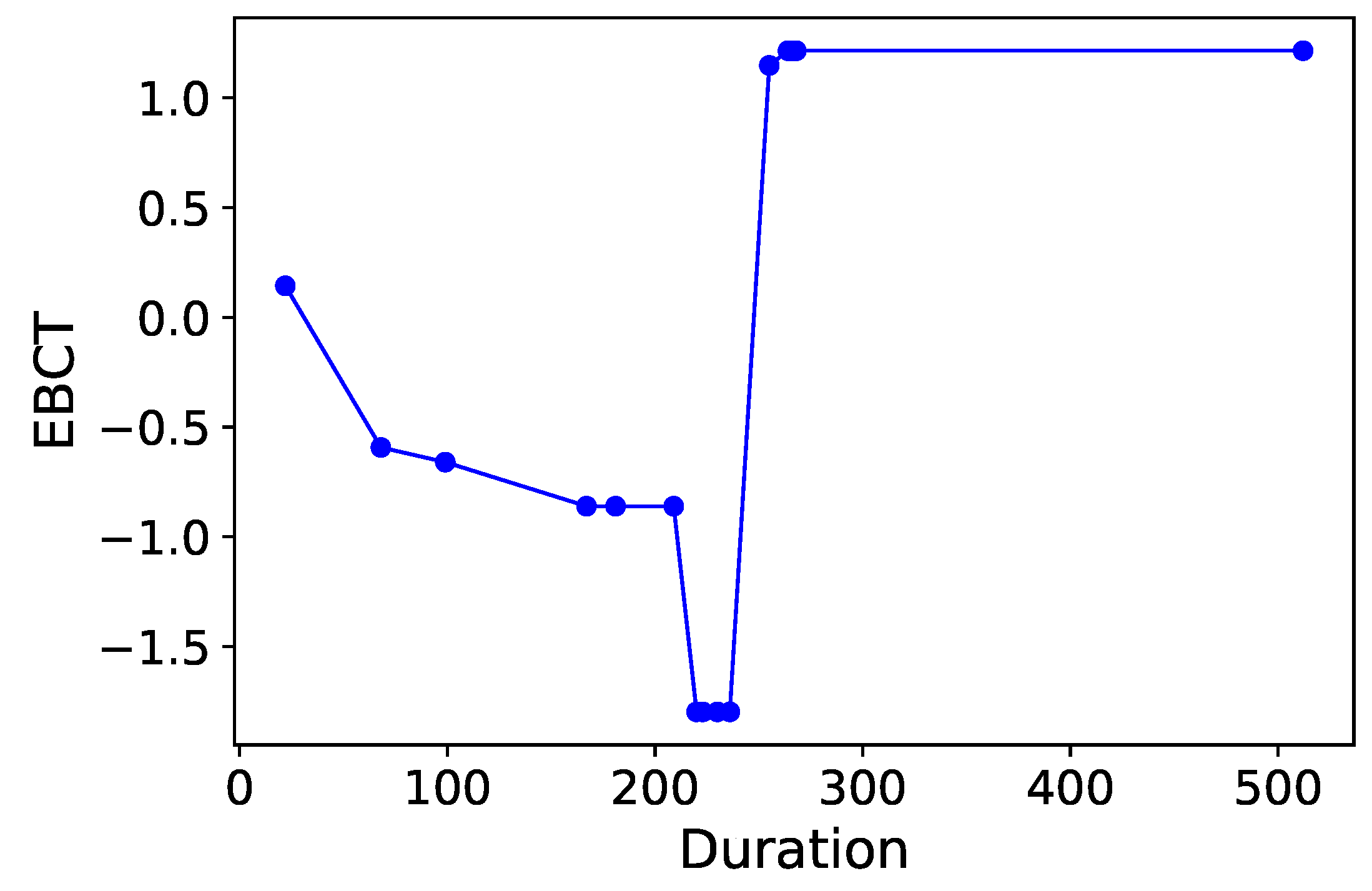
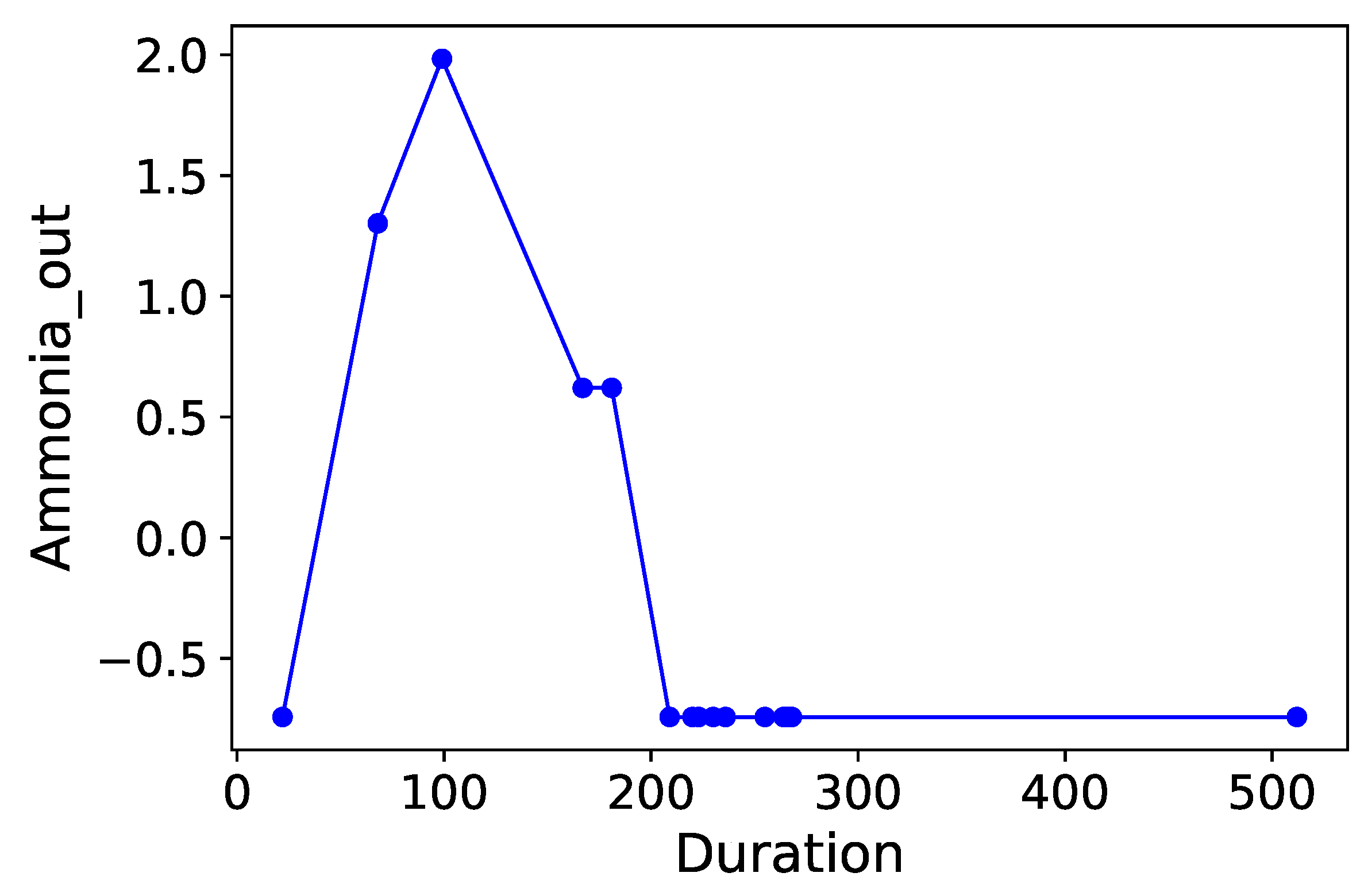
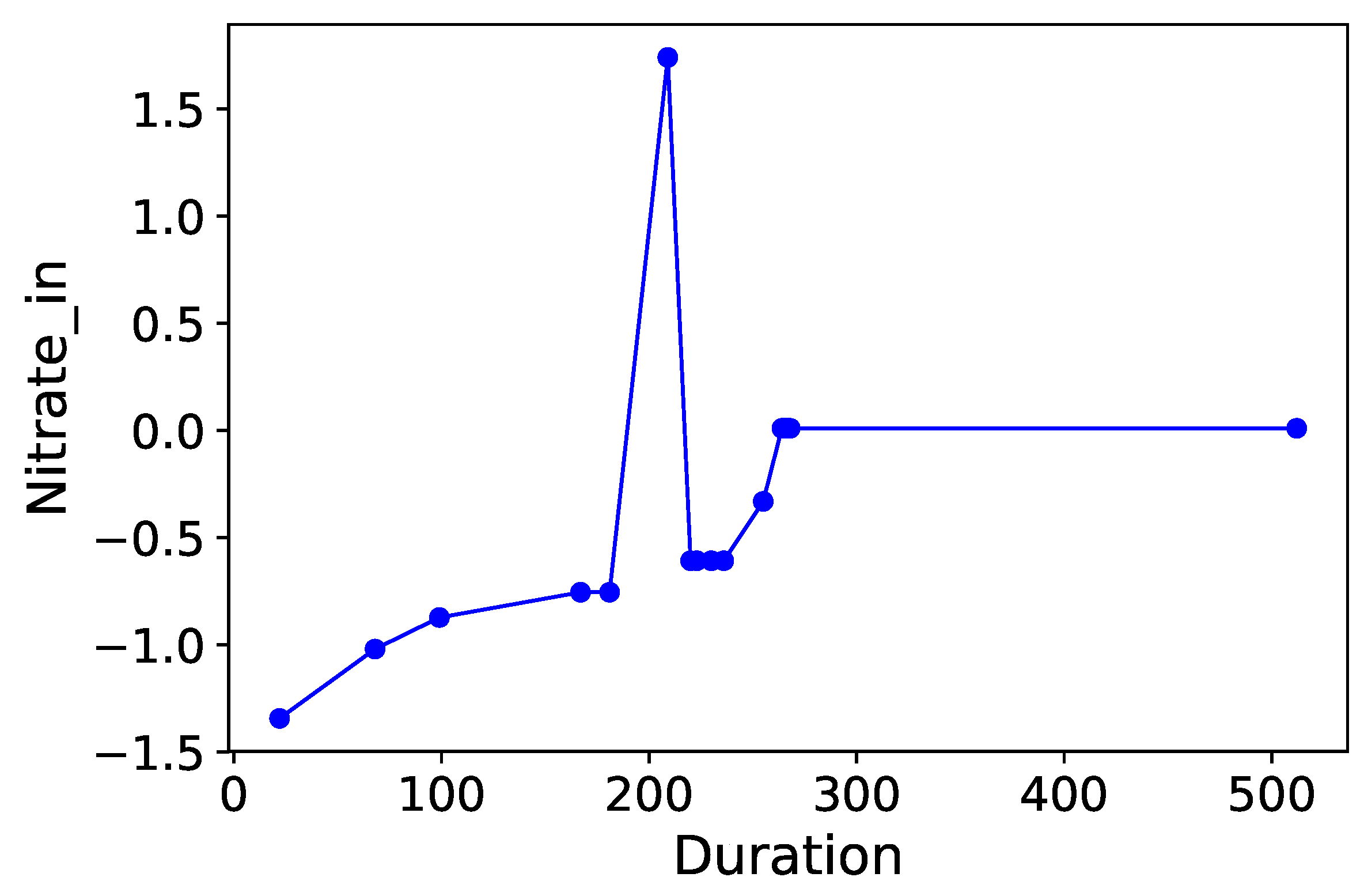
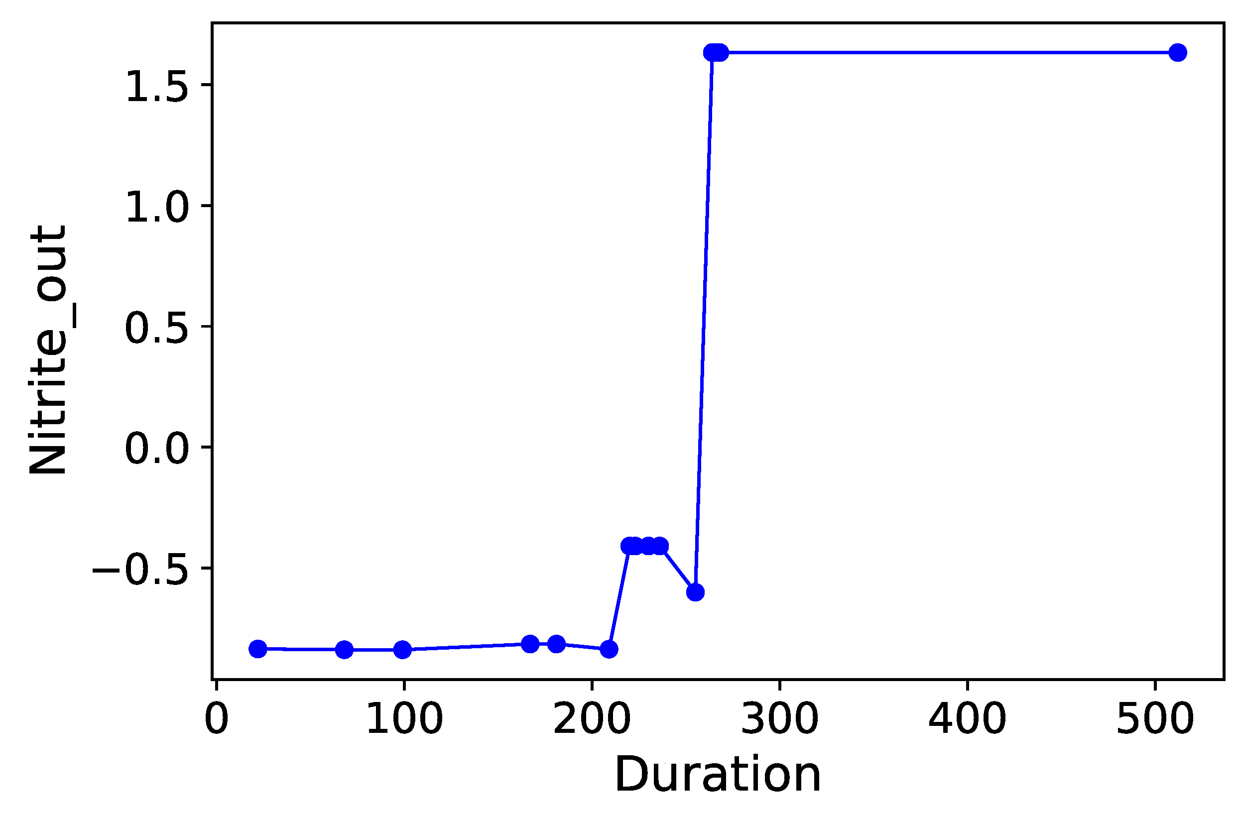
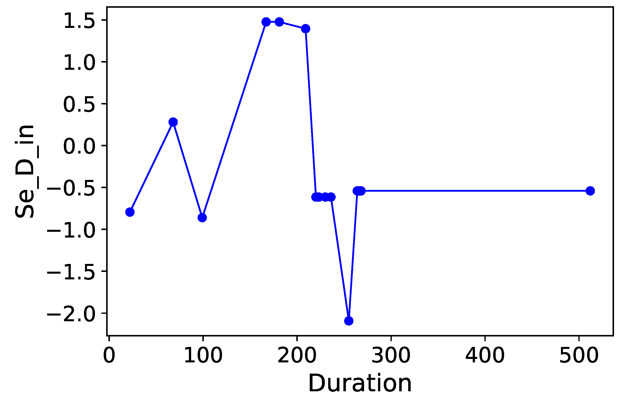
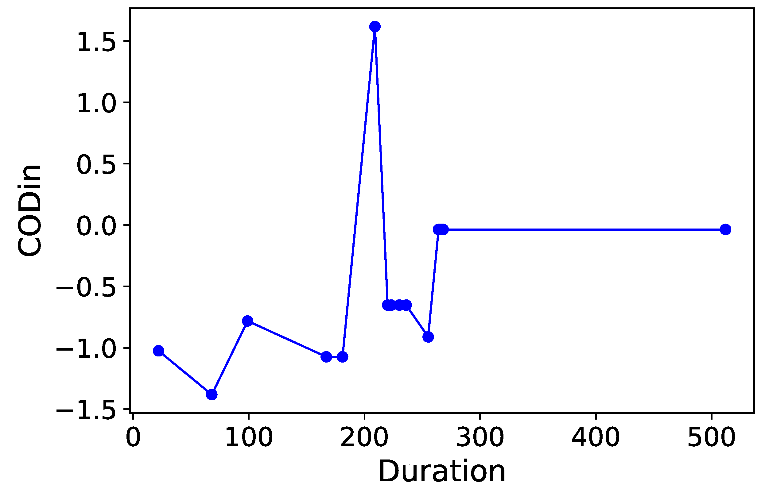
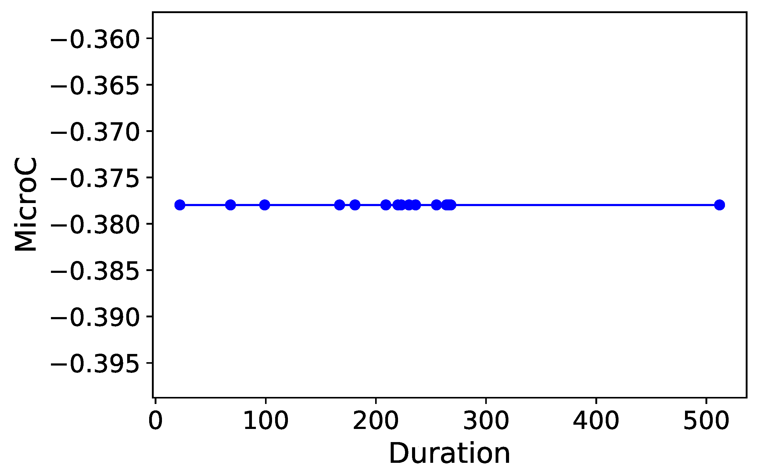
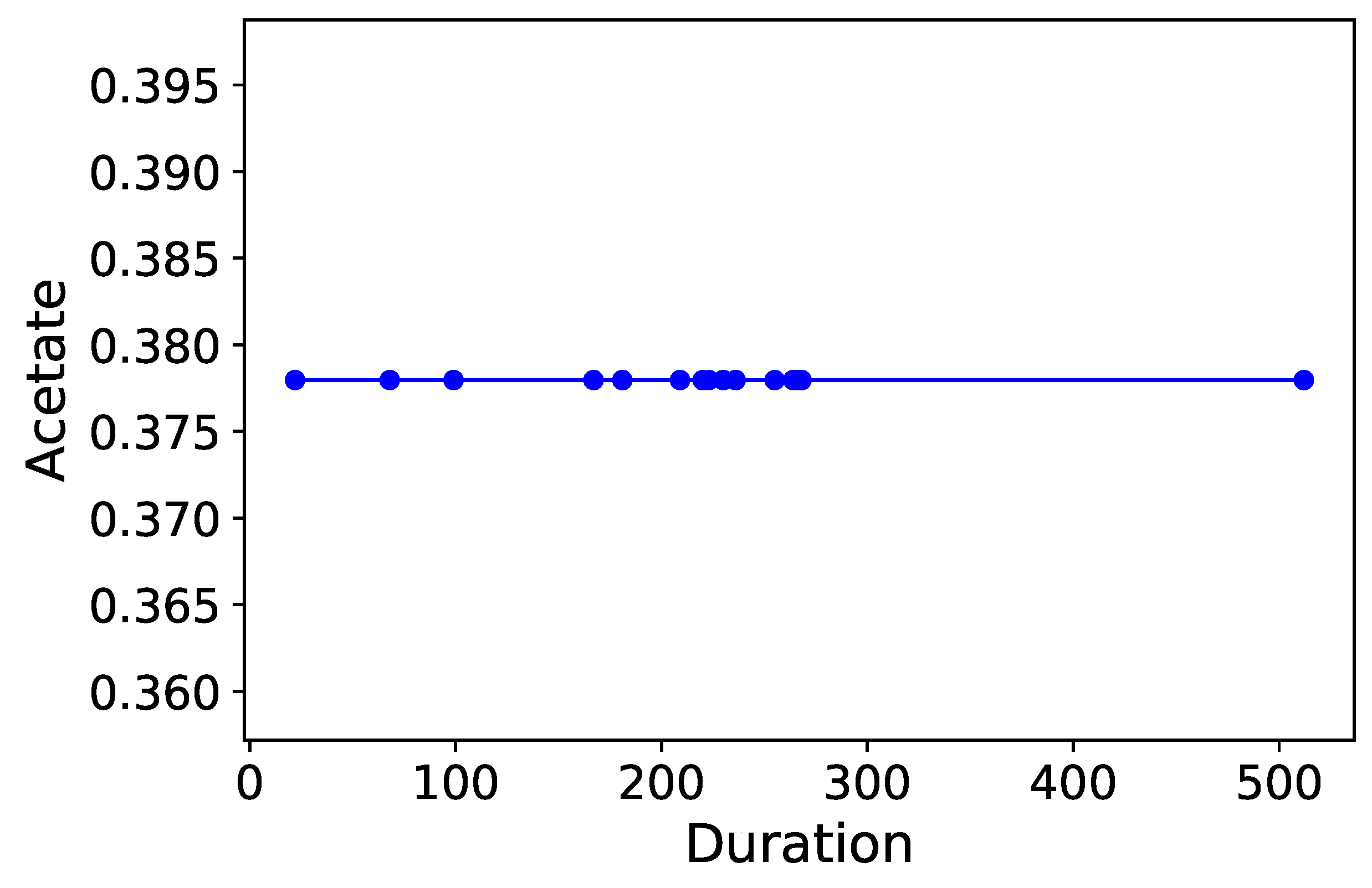
The following sections contain the pertinent results of this case study: clustering, prediction, and feature analysis. The most important part is the comparison of different results obtained from the clustering algorithms, as well as the key variables identified by the feature selection techniques. An overall summary of the results can be found in Section 3.6. Normalized time-plots of each process variable can be found in Appendix K, in Figure A7, Figure A8, Figure A9, Figure A10, Figure A11, Figure A12, Figure A13, Figure A14, Figure A15, Figure A16, Figure A17, Figure A18, Figure A19, Figure A20, Figure A21 and Figure A22. To access the data and code used to generate the results, please visit the main author’s GitHub repository (https://github.com/yitingtsai90/Bioreactor-data-analysis).

3.1. Hierarchical Clustering of OTUs

The $lo{g}_{10}$-transformed counts obtained from pre-processing are first analyzed in terms of biological associations. This provides preliminary knowledge into the possible co-existing and/or antagonistic interactions between OTUs. In order to prevent spurious correlations (which are possible using methods such as Pearson or Spearman correlations), the netassoc algorithm by [30] is used. The result is a 305-by-305 matrix acting as a “pseudo” distance matrix between all OTUs, which can then be used for hierarchical clustering.

Before the netassoc distances can be used, however, it must undergo one final transformation: normalization of values between 0 and 1. This follows the concept of similarity being analogous to small distances (i.e., distances close to zero), and dissimilarity being analogous to large distances. The operation in Equation (2) accomplishes this scaling:

$$\begin{array}{c}\hfill {\mathrm{dist}}_{\mathrm{scaled}}=\frac{\mathrm{dist}-{\mathrm{dist}}_{\min }}{{\mathrm{dist}}_{\max }-{\mathrm{dist}}_{\min }}\end{array}$$

(2)

At this point, the hierarchical clustering models can finally be constructed. First, the following four hierarchical clustering methods are performed on the scaled netassoc distance matrix:

• Unweighted pair-group method with arithmetic means (UPGMA)
• Ward’s minimum variance method (Ward)
• Nearest-neighbour method (Single-linkage)
• Farthest-neighbour method (Complete-linkage)

This was accomplished using the scipy package cluster.hierarchy. In order to determine the “optimal” clustering method out of the four, the cophenetic correlation values (see Appendix H) were obtained using the cluster.cophenet command, for all four methods. The results are shown in

Table 2. Cophenetic (coph.) correlations. Unweighted pair-group method with arithmetic means (UPGMA).

Method	Coph. Correlation
UPGMA	0.51
Ward	0.41
Single-linkage	0.08
Complete-linkage	0.22

.

Cophenetic correlations can be interpreted as how well a clustering method preserves the similarites between raw samples. Since the UPGMA method has the highest cophenetic correlation, it was selected as the most suitable clustering method. A dendrogram was then constructed using this method, and it can be visualized in Figure 8.

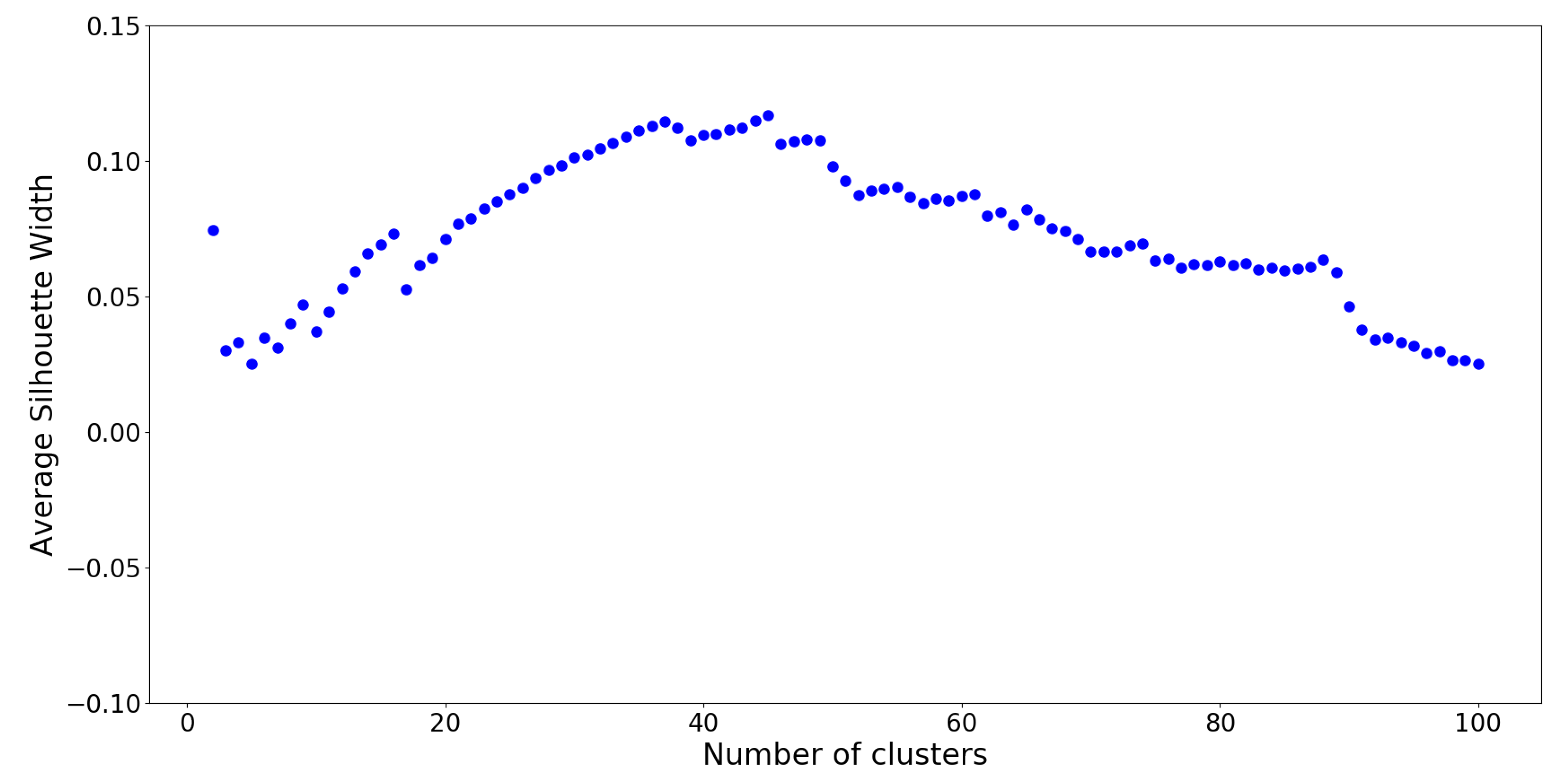
The optimal number of clusters on this UPGMA dendrogram is determined by silhouette analysis (see Appendix H), which is a measure of how well cluster members belong to their respective clusters, given the number of desired clusters K. Silhouette values are computed for cluster numbers $K=2$ through $K=100$, and the results are plotted on Figure 9.

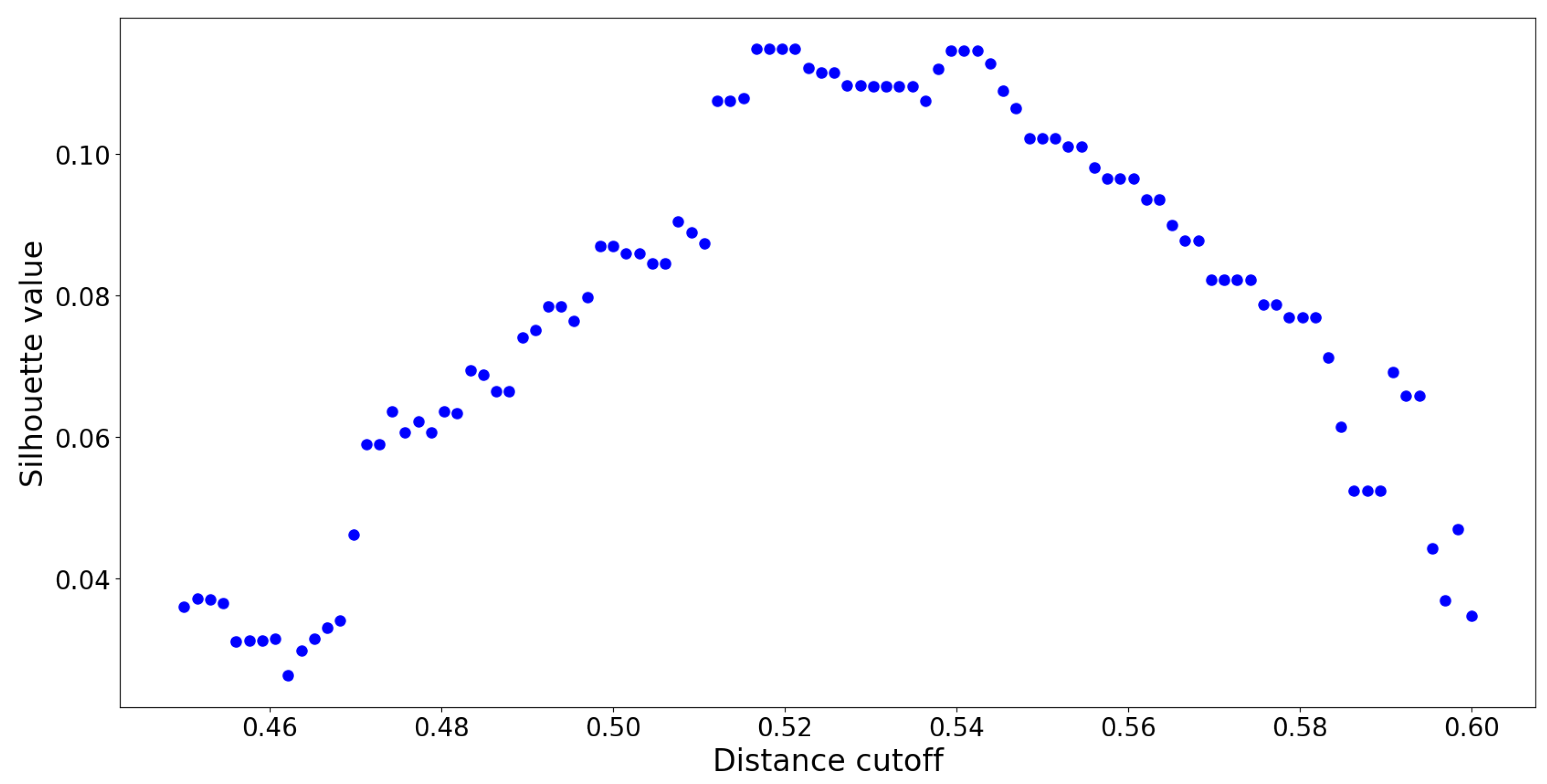
From silhouette analysis, $K=45$ groups appear to be the “optimal” cut-off with the overall highest silhouette value. However, this is assuming that all netassoc distances are suitable for use. Recall that a normalized distance of 0 resembles similarity, and a distance of 1 resembles dissimilarity. A distance of $0.5$ corresponds to neither similarity nor dissimilarity. Values in that vicinity represent “neutral” OTU interactions which act as noise, confounding the clustering model. To remedy this issue, a distance cut-off approach inspired by [36] was employed. If a hierarchy with a distance cut-off value of $dis{t}_{cut}$ is constructed, it means that no cluster contains members which are spread apart by a distance greater than $dis{t}_{cut}$. This reduces the amount of overlap between distinct clusters. To determine the precise value of $dis{t}_{cut}$, several UPGMA hierarchies were constructed using distance cutoffs within the set of values ${\mathit{dist}}_{\mathrm{cut}}\in [0.4,0.6]$. The resulting silhouette values are reported in Figure 10:

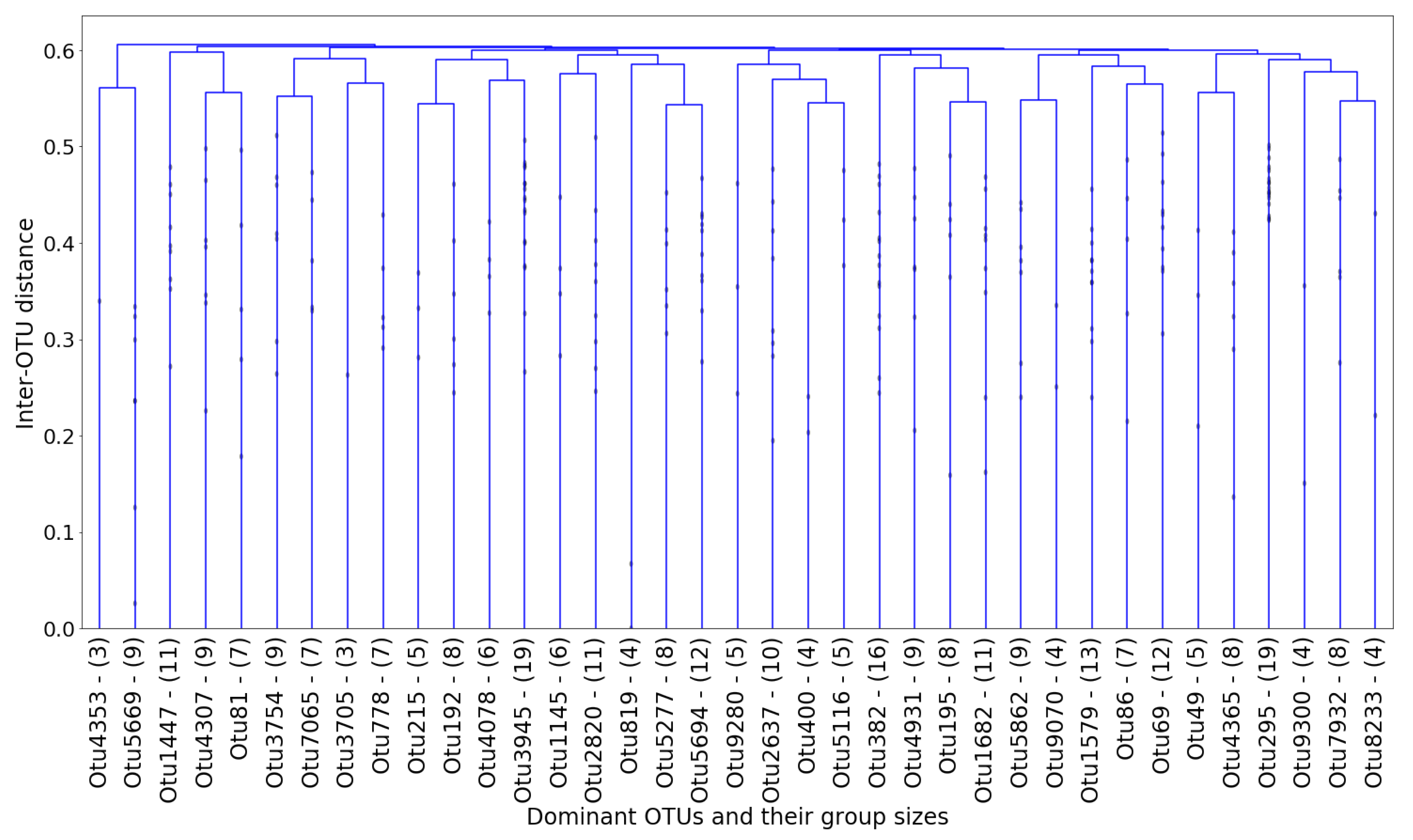
The optimal distance cut-off is located at $0.54$ with a corresponding maximum silhouette value of $0.068$. By constructing a UPGMA hierarchy with this cut-off, no two members within any cluster are spread apart by a normalized distance of $0.54$. This UPGMA hierarchy yields a total of $K=37$ clusters, and its dendrogram is provided in Figure 11:

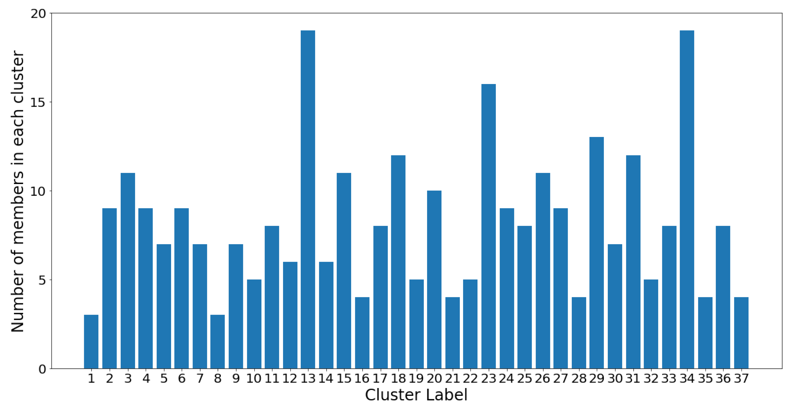
In each cluster, the “dominant” OTU was determined as the one closest (in terms of normalized netassoc distance) to the cluster centroid. The coordinates of each centroid were readily calculated using the distances in the dendrogram. The remaining OTUs in the cluster were therefore considered “followers.” The entire cluster could then be considered a co-existing community of OTUs. In Figure 12, the number of members in each cluster (which is also shown in Figure 11) is plotted against the cluster number.

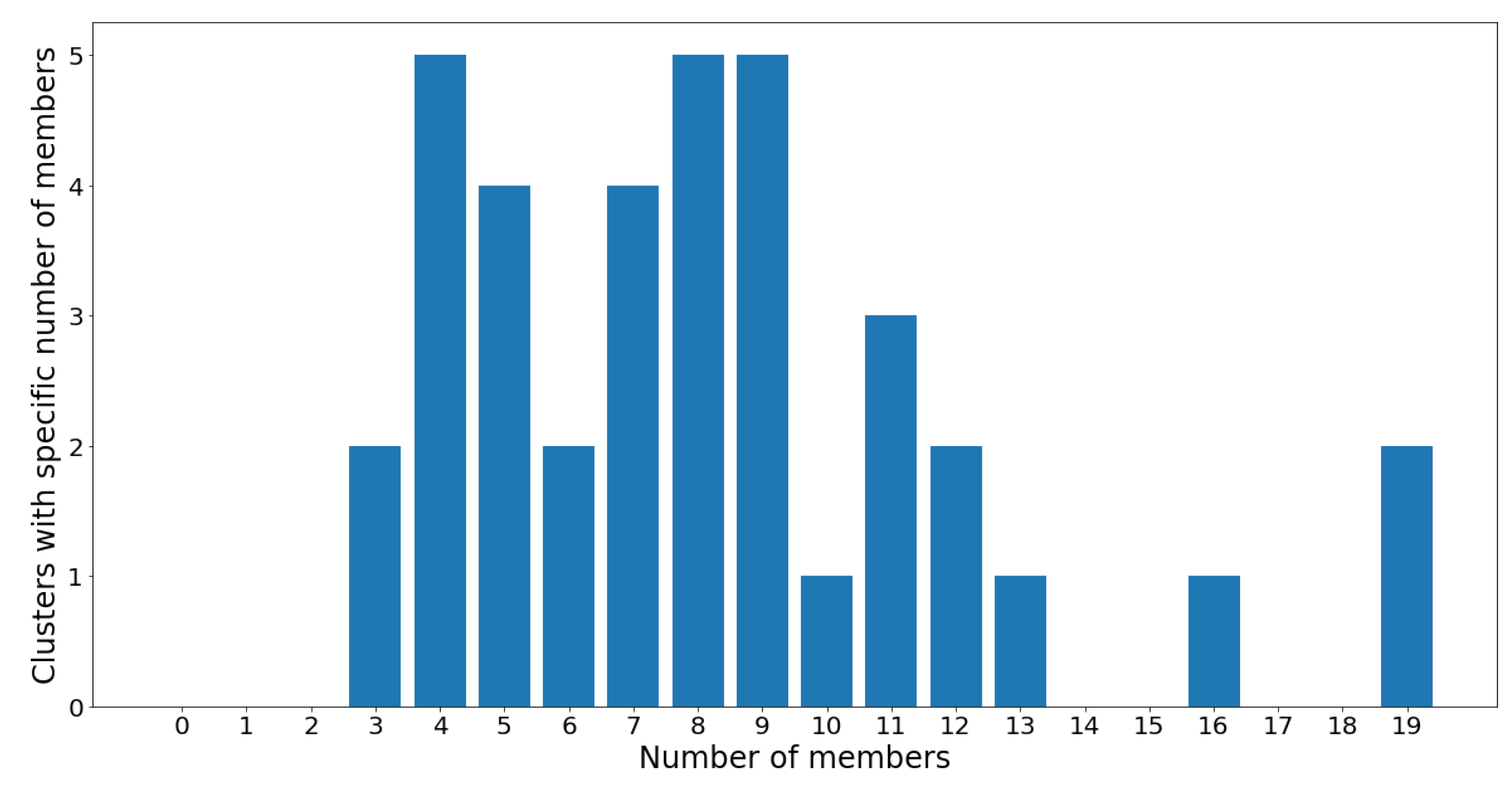
On one hand, clusters 13 and 34 are the largest communities, with 19 OTUs in each. On the other hand, clusters 1 and 8 are the smallest communities, with three OTUs in each, followed by groups 16, 21, 28, 35, and 37 which all contain four OTUs. Despite the considerable variance in community sizes, no communities contain less than three OTUs or more than 20 OTUs. The membership distribution can be observed in the reverse histogram, where the number of groups for each membership size is shown:

Figure 13 shows that most clusters contain four, eight, and nine OTUs, followed by five and seven OTUs. Most clusters have a population ranging between four and 12 OTUs, which indicates a healthy clustering distribution.

For the subsequent prediction and feature extraction steps, only the 37 dominant OTUs shown in Figure 11 are considered, out of the total 305 OTUs to begin with. Although 37 is still a reasonably large number (and not between two and 10, ideally), the choice is based on a combination of statistically-justified methods.

3.2. Gaussian Mixture Analysis of OTUs

Instead of using hierarchical clustering, another possible approach is to group OTUs using gaussian mixture models (GMMs). The assumption here is that the underlying distribution behind the OTU abundances can be modelled as a sum of multivariate Gaussians. Each Gaussian can be considered as a “cluster” of OTUs, with its centroid represented by the mean, and its spread (or size) represented by its variance. The overall GMM is built using the scikitlearn subpackage mixture.GaussianMixture. In order to determine the “optimal” number of Gaussians K, the Akaike information criterion (AIC) and Bayesian information criterion (BIC) values are determined for each value of K. 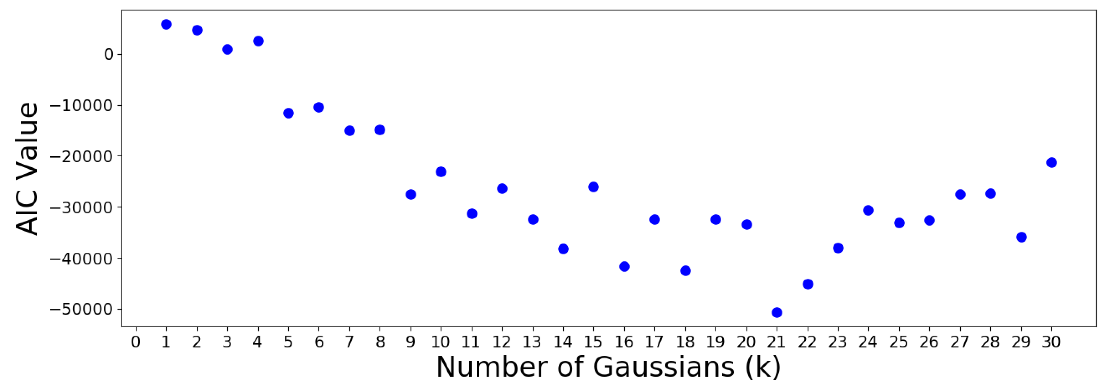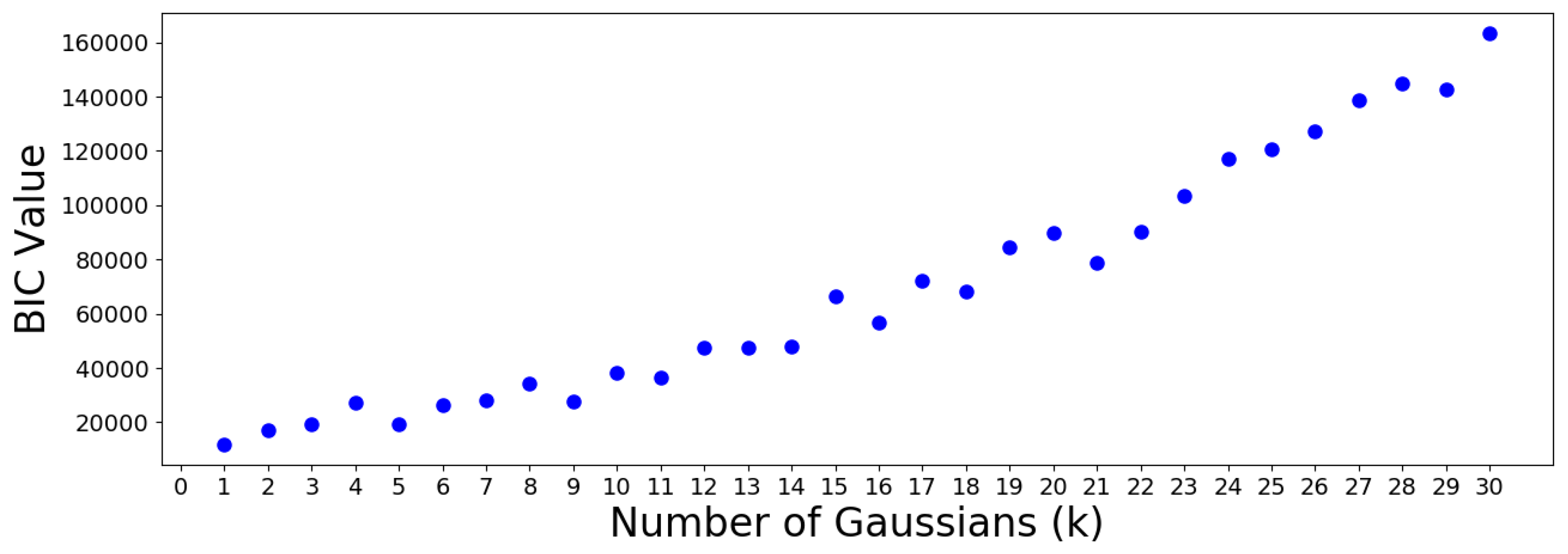This is performed by calling the .aic and .bic attributes of the GMM models within scikitlearn. The results are plotted in the following Figure 14 and Figure 15.

The AIC minimum suggests that the 305 OTUs should be optimally clustered into a GMM with $K=21$ groups. On the other hand, the BIC minimum suggests that a GMM with only one cluster is optimal. This is a meaningless result which should be discarded, since it suggests that all OTUs are similar. Note that the BIC values increase almost monotonically from $K=1$ group onwards, meaning no suitable number of clusters can be determined using this criterion. Therefore, the AIC result is used to move forward.

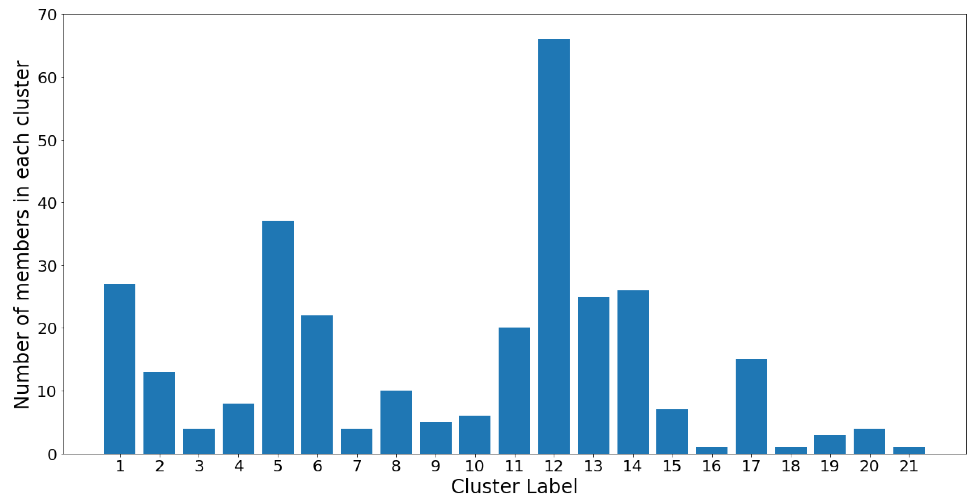
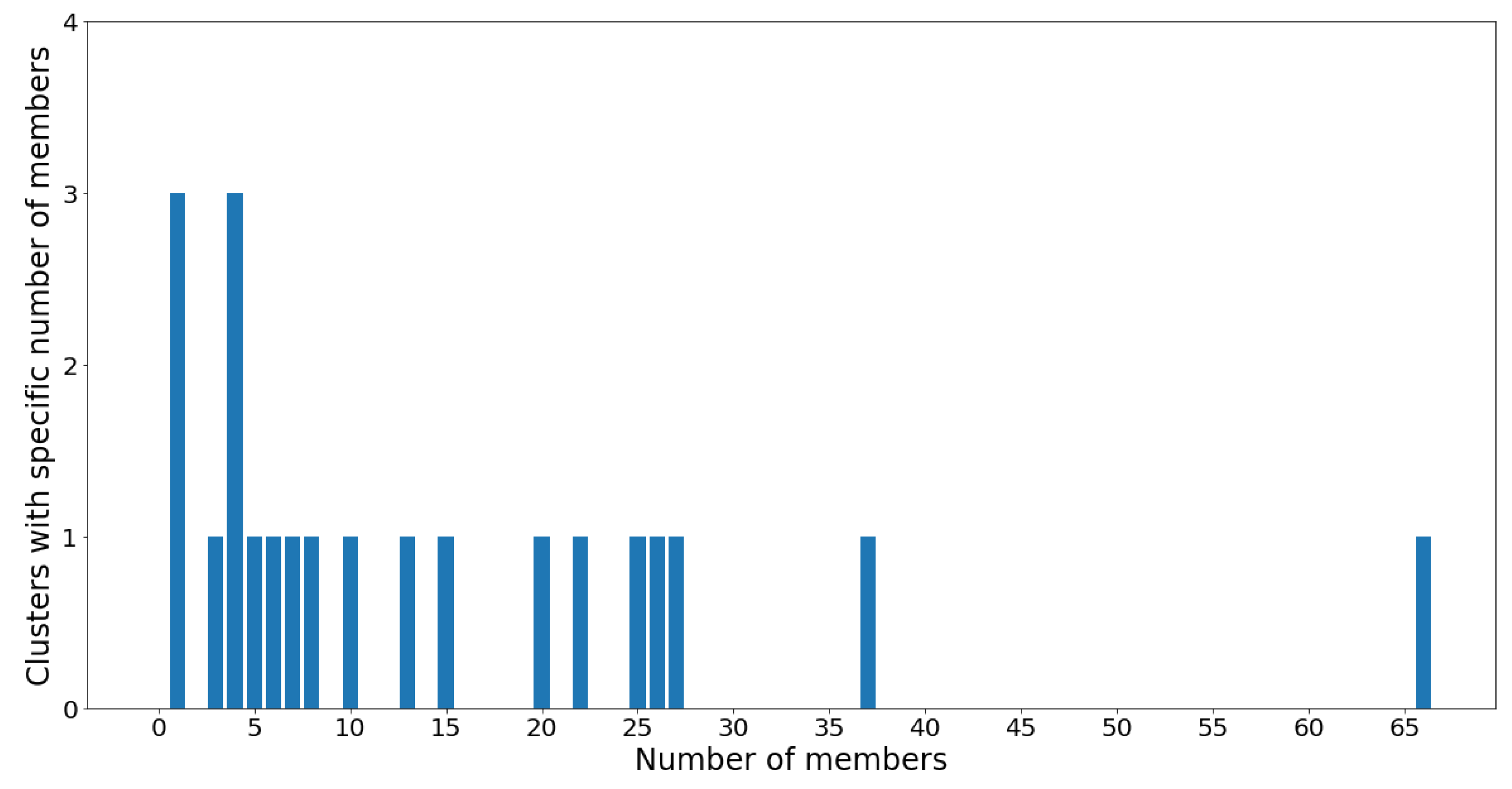
The cluster population and membership plots can be observed in the following Figure 16 and Figure 17.

Notice that the GMM cluster sizes have a much higher variance than the hierarchical clusters. Cluster 12 contains 66 out of the 305 total OTUs, while most other clusters contain between two and 40 OTUs. The skewed nature of the results is most likely due to the log-transformed OTU abundances being skewed towards the low counts. Therefore, the underlying Gaussian assumption (which assumes symmetrical distributions) is inaccurate. Moreover, the Gaussian mixture models were constructed using the abundance counts of OTUs, and not the associations as the hierarchical models were in Section 3.1. These two reasons alone suggest that the Gaussian clusters may not be the best representation of OTU groups. Nevertheless, the results are summarized in

Table 3. Dominant OTUs from Gaussian mixture clusters.

Group Number	Dominant OTU	Group Size
1	OTU200	27
2	OTU46	13
3	OTU11	4
4	OTU112	8
5	OTU3313	37
6	OTU470	22
7	OTU6	4
8	OTU2756	10
9	OTU157	5
10	OTU48	6
11	OTU3057	20
12	OTU185	66
13	OTU559	25
14	OTU778	26
15	OTU8968	7
16	OTU14	1
17	OTU105	15
18	OTU8	1
19	OTU77	3
20	OTU93	4
21	OTU1	1

, which highlights the biomarker OTU in each GMM cluster as well as the cluster size.

3.3. Dirichlet Mixture Analysis of OTUs

In the previous Section 3.2, the OTU abundances were assumed to follow an underlying Gaussian distribution. In light of Figure 4 and Figure 5, this assumption is clearly inaccurate, since even the distribution of log-transformed values appears to be skewed towards the low counts. Therefore, a more suitable assumption for the OTU clusters is the Dirichlet multinomial mixture (DMM) (see Appendix J). Instead of using Python, the Dirichlet Multinomial R package developed by [37] is used. This algorithm is capable of constructing a set of DMM models, assessing the optimal model(s) using AIC, BIC, or Laplace information criterion (LIC), then producing heatmaps of the clustering results based on the Dirichlet weights of each cluster.

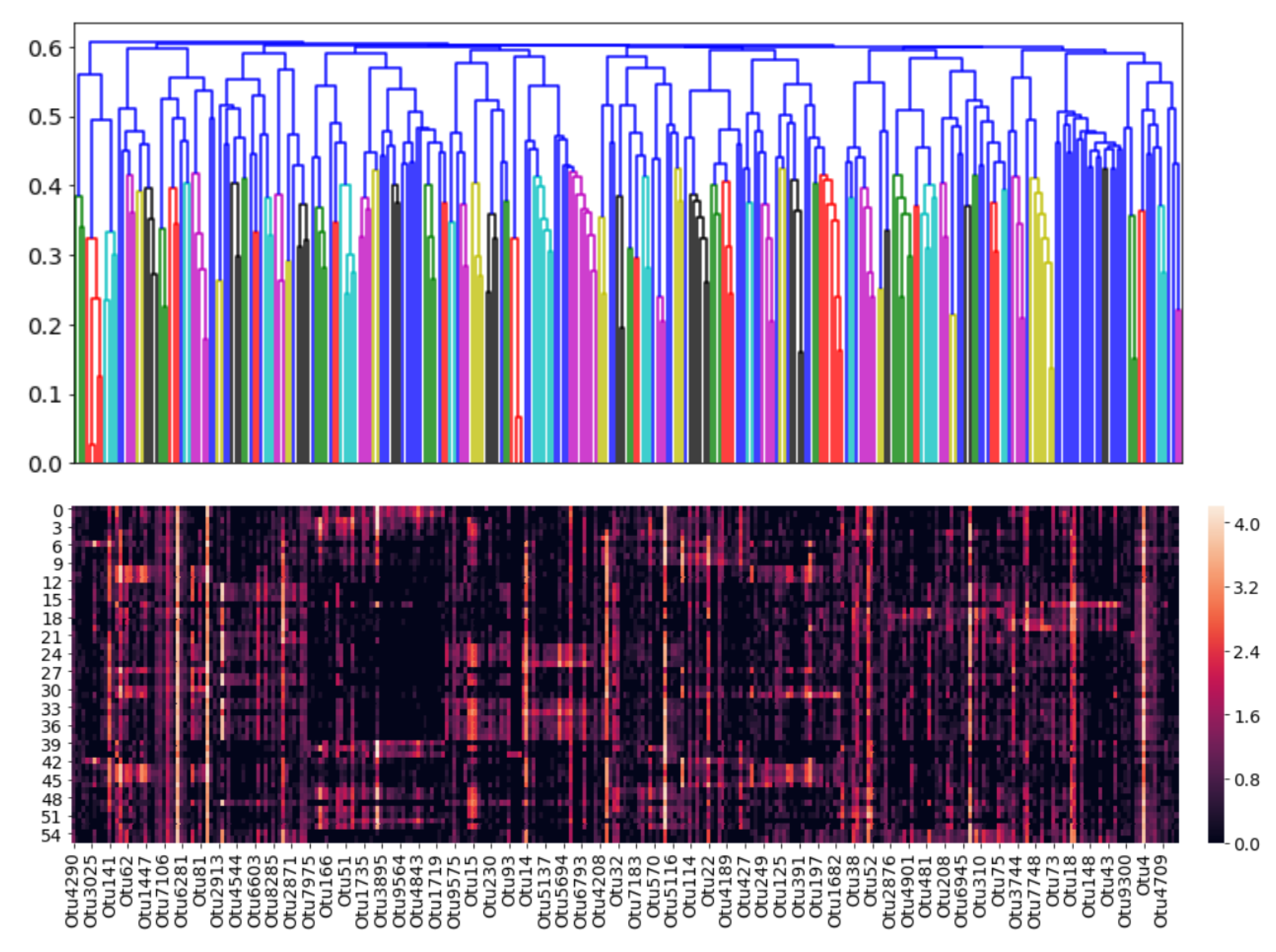
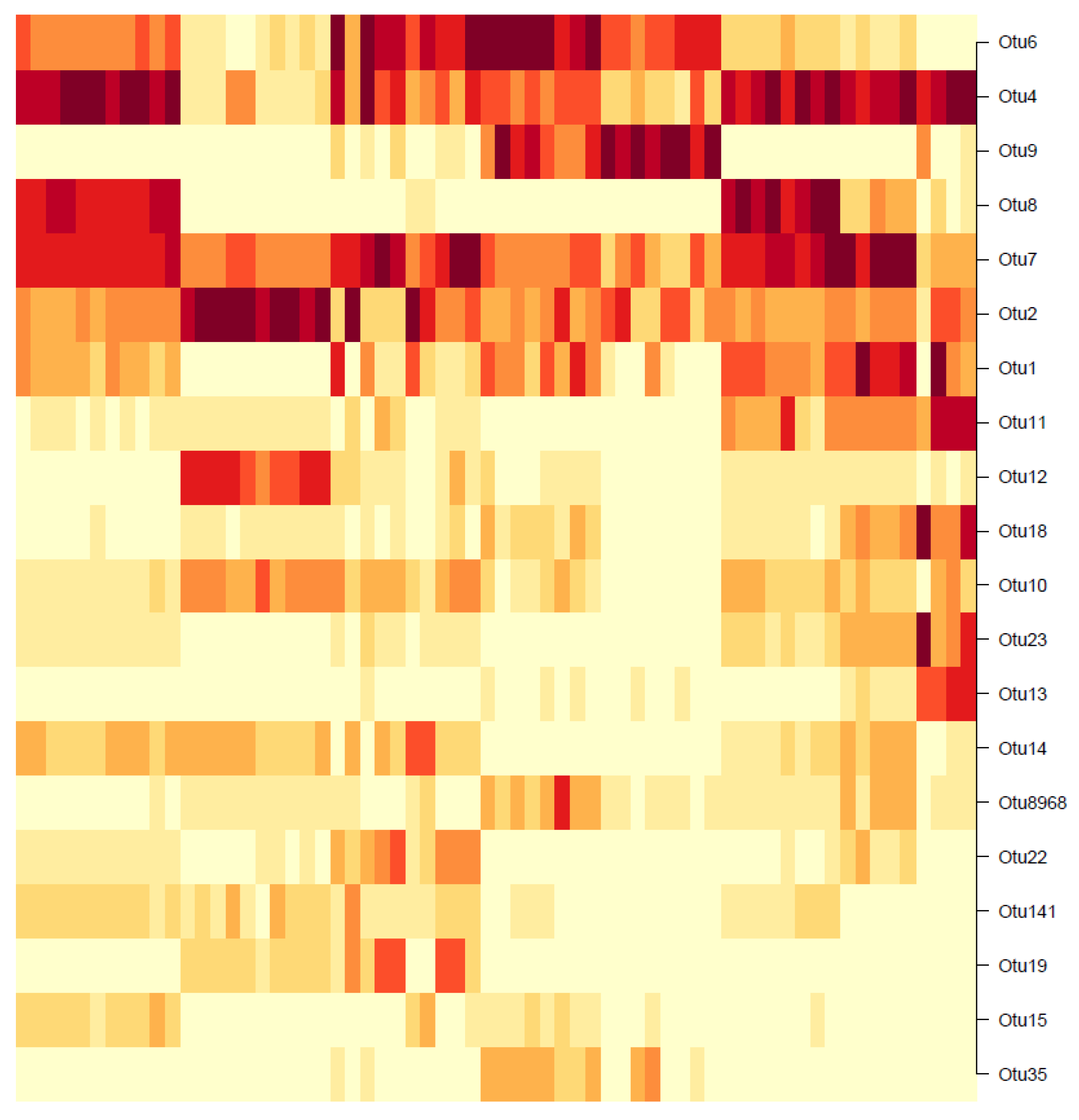
Unlike the hierachical or Gaussian approaches where the clustering is performed on the OTUs and not the samples, the DMM clustering is the exact opposite: The samples are clustered and not the OTUs. The results, however, can still be interpreted to identify the dominant OTUs for further analysis. For the 55 existing samples, the heatmap in Figure 18 shows the BIC-optimal DMM clusters, labelled with the 20 OTUs of highest Dirichlet weights.

Note that the rows of the heatmap represent individual OTUs. In the first row (OTU6), a dark-shaded band exists in the mid-samples, including a commonly high abundance of OTU6 in those samples and low abundances elsewhere. Similarly, for the second row (OTU4), a common high-abundance band is observed for the first and last few samples, with low abundances elsewhere. This visual result reinforces the concept that the DMM model clusters the individual samples (columns) and not the OTUs. However, notice that going down the heatmap from OTU6 to OTU35, the dark- shaded bands appear less frequently. The colours become increasingly white, indicating an overall decrease in OTU abundance. Below the 20th-OTU cutoff (of OTU35), the rows are entirely white with close to zero abundance, and therefore those results have been truncated from the figure. Therefore, the 20 OTUs shown in Figure 18 are considered as the biomarker OTUs, akin to those in the hierarchical and GMM clustering results. However, the followers of these 20 biomarker OTUs cannot be determined, since the clustering was not performed OTU-wise.

3.4. Prediction Results

The 10 water chemistry variables (outlined in Table 1) are combined with representative OTUs obtained from Section 3.1, Section 3.2 and Section 3.3. Together, these serve as inputs. When combined with the corresponding, labelled process outcomes of selenium removal rate (SeRR), predictive models are trained for the estimation of the SeRR of new samples.

The models can be categorized in terms of their inputs, as follows:

• Base case: Water chemistry variables only.
• Hierarchical: Water chemistry variables plus representative OTUs obtained using hierarchical clustering.
• Gaussian: Water chemistry variables plus representative OTUs obtained using GMMs.
• Dirichlet: Water chemistry variables plus representative OTUs obtained using DMMs.

The idea is to observe whether the addition of biological features improves or confounds the predictive capabilities of these models. The actual models consist of the following three types:

• Random forests (RFs)
• Support vector machines (SVMs)
• Artificial neural nets (ANNs)

The raw SeRR values obtained from plant data were normalized and discretized into two (binary) classes, 0 and 1. Class 0 (poor) corresponds to SeRR values which fall below the mean SeRR, and Class 1 (satisfactory) corresponds to values above the mean. Out of the $N=56$ total data samples, 29 have a class label of 0 and 27 have a class label of 1, therefore the overall distribution is fairly even (i.e., not skewed towards one label).

For each model, $40\%$ of samples from each class are randomly selected as test samples for performance assessment, and the remaining $60\%$ of samples as training samples for model construction. Note that this approach eliminates the possibility of biased selection from either class. If the training and testing sets were instead selected arbitrarily from the entire dataset, then they could possibly be skewed (e.g., many samples selected from Class 1, but few from Class 0).

No validation (development) set was required, since the hyperparameters of each model (i.e., regularization constants, model complexity, etc.) were selected to be fixed values for simplicity. The RF model was constructed using the RandomForestClassifier module from scikitlearn.ensemble, with bootstrapping disabled. Although bootstrapping is normally recommended, the data sample-size in this case $(N=56)$ is extremely small for modeling purposes. Therefore, all of the existing $56\times 0.6\simeq 34$ samples are required for training; any arbitrary selection of samples without replacement could skew the training set. The SVM model was constructed using the sklearn.svm.svc module, with a regularizer value of $C=1$ and the default linear kernel. Finally, the ANN model was constructed using tensorflow, with 10 layers of 20 neurons each, a learning rate of $\alpha =0.01$ and a ${\ell }_2$-regularizer of $\lambda =0.1$. In order to maintain the reasonable computational times required by each model, a maximum of 1000 epochs (or “outer iterations”) were allowed. The ANN model was allowed 50 steps (or “inner iterations”) per epoch.

The prediction accuracy of each model on the test set (of $56\times 0.4\simeq 22$ samples) is reported in

Table 4. Prediction results for each model type. Random forests (RFs), support vector machines (SVMs), and artificial neural networks (ANNs).

	Base Case	Hierarchical	Gaussian	Dirichlet
RF	$96.3$	$90.6$	$93.4$	$92.2$
SVM	$91.8$	$87.2$	$91.3$	$90.6$
ANN	$81.7$	$78.6$	$83.4$	$80.2$

, with respect to the type of inputs used.

The RF models produced the most accurate test predictions for every case, followed by SVMs then ANNs. When comparing the input types, the base case accuracy turned out to be the highest for both RF and SVM models. The addition of hierarchical OTU clusters had the largest detrimental effect on the test accuracy, as observed by the uniform, marked decreases across all three model types. The addition of Gaussian OTU clusters improved the test accuracy for the ANN model, but proved to be detrimental for the RF and SVM models, albeit with the least impact. The addition of Dirichlet OTU clusters also decreased the model accuracy for all three models, but not as much as the hierarchical. These results clearly show that the addition of biological data, which was initially expected to improve quality of prediction, actually degrades it. Even though the OTU abundances should contain valuable insight into the biological community interactions, the observed confounding effect is most likely due to the undesirable qualities of the data. These include the inherent noise present in the OTU abundances, and also the relatively low sample size $(N=56)$ to begin with. Another reason could be that the explored clustering methods are incapable of clearly extracting information related to coupling effects between OTUs and water chemistry variables.

If a model were to be selected for actual prediction of process outcomes, it would be the RF using base-case, water chemistry variables. This model achieves a respectable >$95\%$ accuracy on the binary classification of SeRR.

3.5. Feature Selection Results

The relevant features in the prediction framework are defined as those which contribute significantly to the accuracy of the model. The results in Section 3.4 showed the RF model as the most accurate one out of the three modeling approaches, and therefore it will be used for feature analysis in this section. The univariate feature selection strategy, mean decrease in accuracy (MDA), was first used to determine “relevant” features in terms of predicting the outcome $SeRR$. An RF model was constructed for each of the input types of hierarchical, Gaussian, and Dirichlet clustering. 10,000 permutations of MDA were performed for each RF model; the averaged feature importances for each are summarized in the following

Table 5. Mean decrease in accuracy (MDA) feature importances for hierarchical clustering.

Feature	MDA $(\%)$
$S{e}_{D,in}$	6.3
$Ammoni{a}_{out}$	0.3
$EBCT$	0.2
$Nitrit{e}_{out}$	0.2
OTU215	1.5
OTU2637	0.6
OTU1579	0.6
OTU49	0.6
OTU3945	0.5

,

Table 6. MDA feature importances for Gaussian clustering.

Feature	MDA $(\%)$
$S{e}_{D,in}$	7.1
$EBCT$	1.2
$Ammoni{a}_{out}$	0.7
$Nitrit{e}_{out}$	0.7
OTU57	1.5
OTU7347	1.1
OTU2765	0.9
OTU48	0.9
OTU7	0.8

and

Table 7. MDA feature importances for Dirichlet clustering.

Feature	MDA $(\%)$
$S{e}_{D,in}$	5.3
$EBCT$	1.9
$Nitrit{e}_{out}$	1.1
$CO{D}_{in}$	0.7
OTU35	1.4
OTU8	1.0
OTU7	1.0
OTU1	0.6
OTU9	0.5

. Only the top four water chemistry and top five OTU features are reported for conciseness.

Notice that $S{e}_{D,in}$ consistently appears in each table as the most “relevant” feature, as MDAs of $5\%$∼$7\%$ are observed as this feature is permutated. $EBCT$ appears to be the second contender, causing accuracy drops of $1\%$∼$2\%$ in most cases when permutated. $Ammoni{a}_{out}$ and $Nitrit{e}_{out}$ are the next most “relevant” features, however permutating them causes smaller accuracy drops of $(<$$1\%)$ on the RF models. Therefore $S{e}_{D,in}$ and $EBCT$ can be comfortably concluded as the main deciders of overall selenium removal rate, in terms of all water chemistry variables. This result is logical from a domain-knowledge perspective, since both variables are used for selenium removal rate calculations using a mass-balance approach.

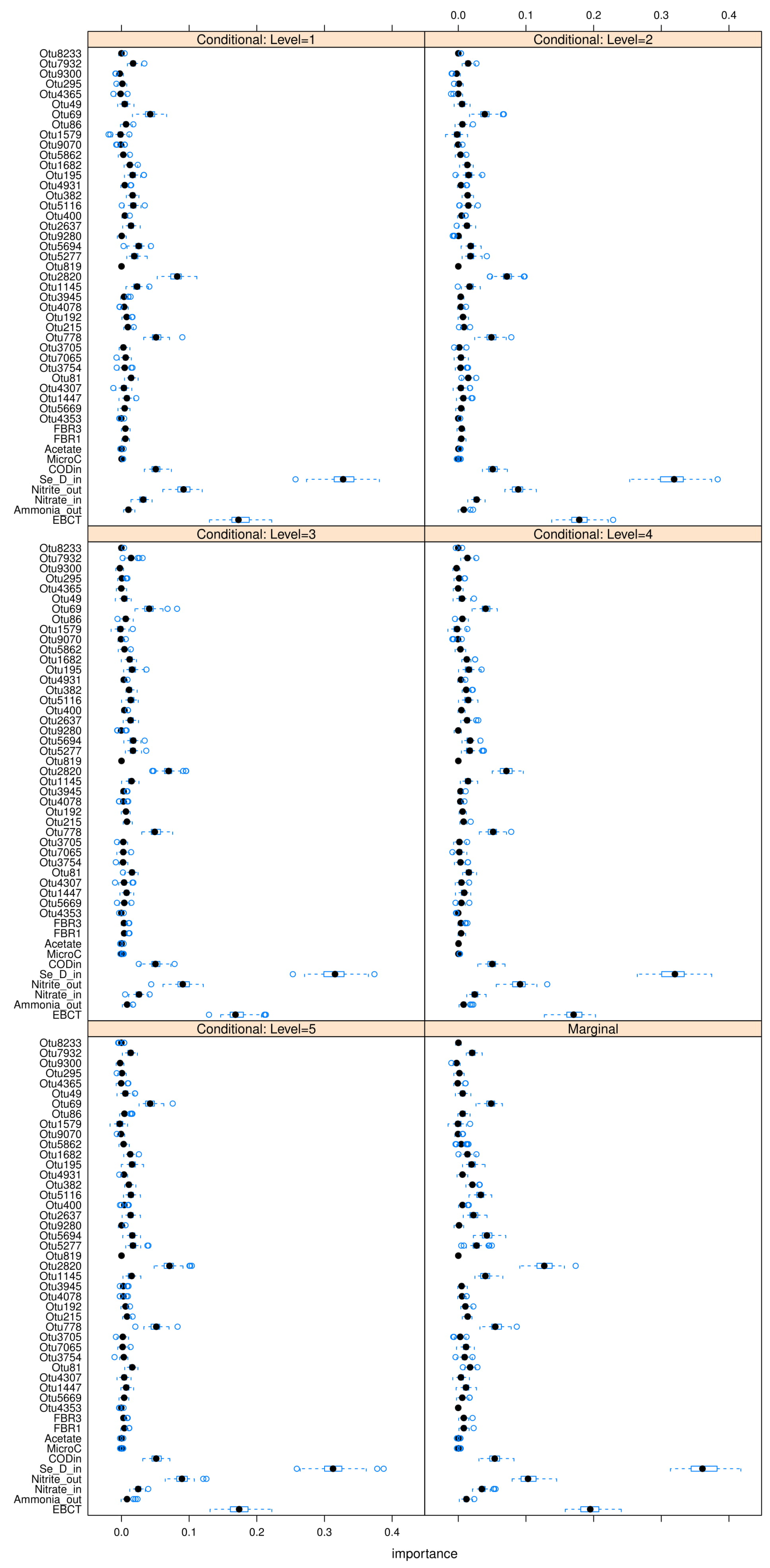
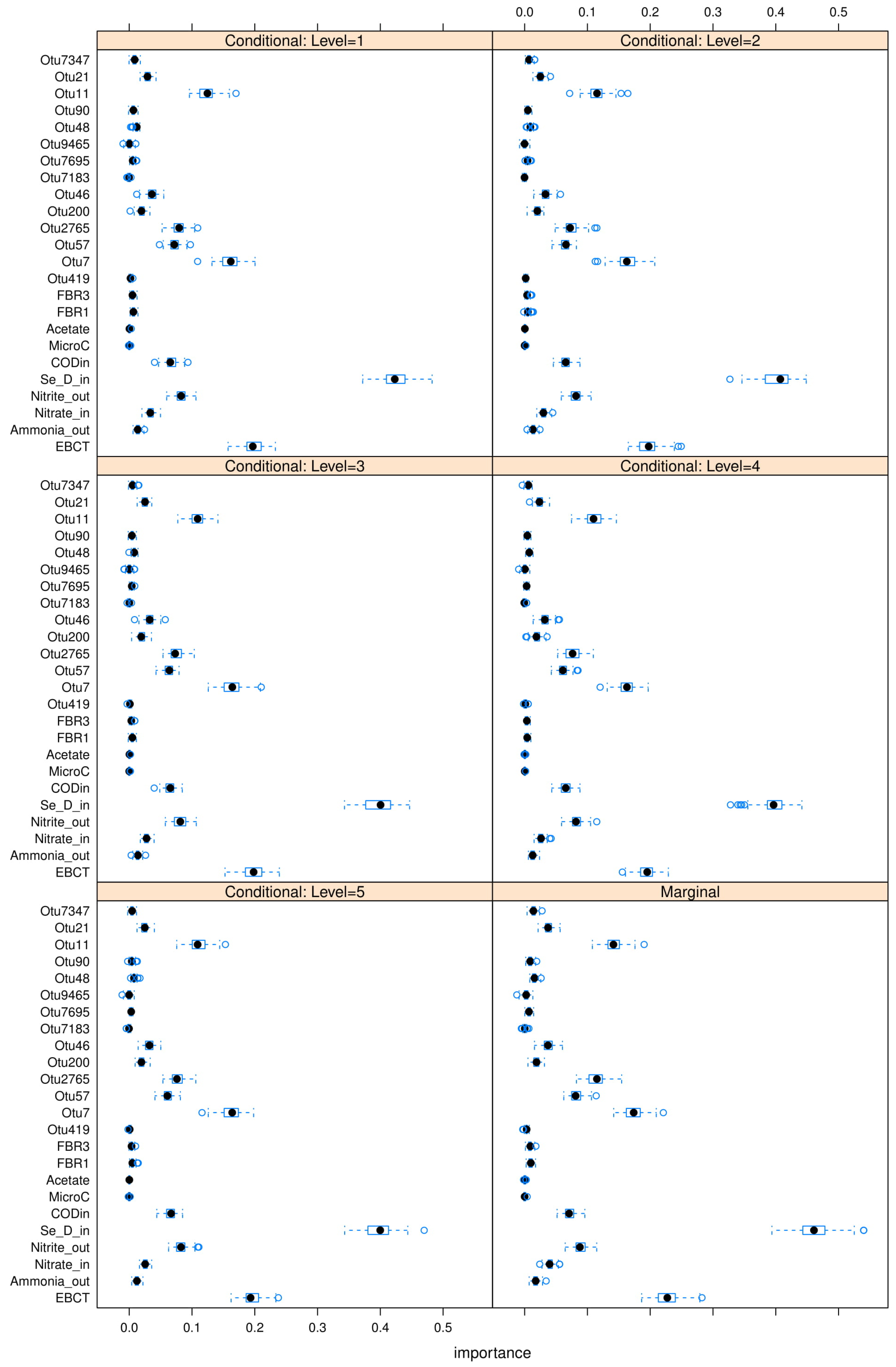
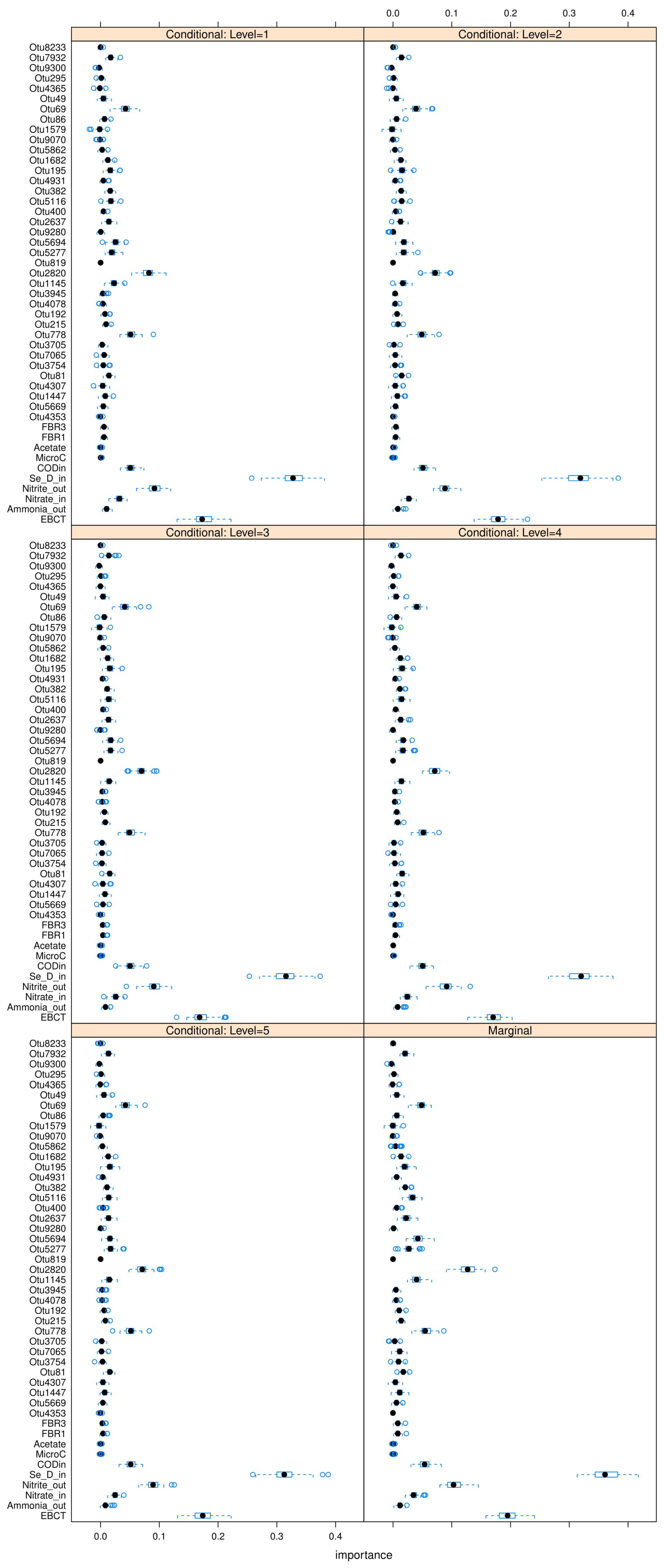
Note that the MDA approach is univariate, which means it ignores possible correlations between multiple features. In order to address this issue partially, the conditional mean decrease in accuracy (C-MDA) approach is also explored. In C-MDA, the permutations of features are performed, given the presence of other features. For example, when the feature $S{e}_{D,in}$ is permutated, it is conditioned on the fact that the feature $EBCT$ falls within a certain bracket of values. The R package developed by [35] is used to perform these C-MDA experiments, since the algorithm systematically decides the best values for the secondary variables to be conditioned upon. The detailed results can be found in Figure A23, Figure A24 and Figure A25 in Appendix L. The “relevant” variables from each RF model can be summarized in

Table 8. Overall Conditional Permutation feature importances.

Rank	Feature
1	$S{e}_{D,in}$
2	$EBCT$
3	$Nitrit{e}_{out}$
4	$CO{D}_{in}$
5	$Nitrat{e}_{in}$
6	$Ammoni{a}_{out}$

:

3.6. Summary and Critique of Results

Of the supervised learning techniques tested, Section 3.4 show that RFs were the best model in terms of test-set accuracy, followed by SVMs and ANNs. RFs are an ensemble method which averages the predictions from a large number of randomly constructed models, as opposed to the SVMs or ANNs which were constructed in one shot. The ANNs performed the worst, due to the fact that deep learning models typically require an exorbitant number of samples (e.g., millions) to predict well, and only 56 samples were available in the dataset.

Inconsistent results (Section 3.1 and Section 3.2) were obtained for biomarkers identified through the three unsupervised techniques. This is due to two reasons: First, assocation values were used for hierarchical clustering, while abundance counts were used for the Gaussian and Dirichlet mixtures. Secondly, the three clustering methods also differ significantly from a statistical perspective. Specifically, the hierarchical clustering was based on pair-wise similarity calculations, whereas the Gaussian mixtures modelled OTU groups as a sum of overlapping distributions. The Dirichlet mixtures are distinct from the previous two clustering methods, since they were calculated using the 56 data sample rows rather than the 305 OTU columns. When modeling OTUs using multinomial distributions, an OTU can occur in several different groups associated with different operating stages or levels of process performance. This may be a closer representation of reality, instead of constraining each OTU to belong to one particular group only. Evidence supporting this conclusion includes, for example, the low Silhouette values (i.e., qualities of clusters) shown in Figure 9 and Figure 10.

Finally, the feature selection results are also quite nuanced. Specifically, note that $S{e}_{D,in}$ and $EBCT$ were identified as key variables in Table 5, Table 6 and Table 7. These are obvious contributory features from a domain knowledge perspective, since their numerical values directly determine the selenium removal rate. Non-obvious features such as $Ammoni{a}_{out}$, $Nitrit{e}_{out}$, and ${COD}_{in}$ are also identified as important. Surprisingly, however, the carbon source variables $Acetate$ or $MicroC$ are never identified as contributory features. The type of carbon source is known to directly impact microbial community compositions in other studies (such as [38]), and therefore they were expected to influence selenium removal significantly. Finally, note that $OTU215$, $OTU57$, and $OTU35$ have been identified as key biomarkers of high importance in Table 5, Table 6 and Table 7. Their feature importances are higher than several of the top four process variables in each case, which reinforces the hypothesis that microorganisms do in fact noticeably affect final selenium removal rate. Interestingly, $OTU7$ appears as an important feature in both Gaussian and Dirichlet clusters, which are two models with entirely different statistical assumptions and properties. However, note that these biomarker OTUs represent clusters, which may be a sub-optimal way of characterizing the true OTU interactions. The clarity and robustness of these results can be improved, for example, by modeling OTUs as individuals rather than agglomerates. A possible avenue in this direction is explored in the following Section 4, and is recommended as a follow-up study to this work.

4. Conclusions and Future Work

The main objectives of this work are as follows: To compare the prediction capabilities of three predictive models (RFs, SVMs, and ANNs), as well as the abilities of three clustering methods (hierarchical, Gaussian, and Dirichlet mixtures) and two feature selection techniques (MDA and C-MDA) to identify key process variables. On one hand, the main process outcome of the selenium removal rate was observed to be best predicted by RF models. The obvious features of selenium loading and retention time were both identified as key contributors to the selenium removal rate. Non-obvious features such as ammonia outflow, nitrite outflow, and chemical oxygen demand were also identified as contributors, but surprisingly these exclude carbon source (a known factor which significantly alters OTU communities). On the other hand, the three clustering methods identified several different biomarker OTUs, which had feature importances similar to those of the aforementioned process variables. This result supports the notion that the OTUs play a substantial role in the removal of selenium from the bioreactor.

The results of this study suggest many possible avenues for future work. In terms of predictive modeling, the small-N issue can be mitigated by building a data simulator, which generates artificial samples based on the existing data. This can be accomplished by adapting the use of generative adversarial nets (GANs) [39], which is popular in image datasets. If a sufficient number (e.g., thousands) of samples are generated, then neural nets with much higher prediction accuracies can be constructed. The parameters as well as architecture of the neural nets can both be adaptively updated on each iteration, using the stochastic configuration network (SCN) method established by [40]. This method has demonstrated success in similar wastewater treatment applications such as [41,42,43].

In order to extract clearer conclusions from the biological data, the unsupervised learning paradigm can be changed from clustering models to graphical models. Instead of forcing the OTUs into clusters that they may not sensibly belong to, an alternative is to use Bayesian networks [31] for causality analysis. In this approach, the OTUs are instead modelled as individual entities or states, as nodes on a graph. The interactions between OTUs are modelled by state-transition probabilities, or graph edges, instead of overlapping clusters. Root-cause identification can then be performed by tracking the graph backwards from the process outcome (the last event) to the key trigger(s) at the start. This strategy has seen success in [44], as well as in the alarm management literature by [45,46] using Granger causality. A follow-up paper could explore the efficacy of these suggested methods, by identifying new OTU biomarkers using graphical models and observing whether they contribute more to the predictive models (in Table 4).

References

1. Breiman, L. Bagging predictors. Mach. Learn. 1996, 24, 123–140. [Google Scholar] [CrossRef] [Green Version]
2. Cortes, C.; Vapnik, V. Support-vector networks. Mach. Learn. 1995, 20, 273–297. [Google Scholar] [CrossRef]
3. Cutler, D.R.; Edwards, T.C., Jr.; Beard, K.H.; Cutler, A.; Hess, K.T.; Gibson, J.; Lawler, J.J. Random forests for classification in ecology. Ecology 2007, 88, 2783–2792. [Google Scholar] [CrossRef]
4. Campbell, W.M.; Campbell, J.P.; Reynolds, D.A.; Singer, E.; Torres-Carrasquillo, P.A. Support vector machines for speaker and language recognition. Comput. Speech Lang. 2006, 20, 210–229. [Google Scholar] [CrossRef]
5. Rumelhart, D.E.; Hinton, G.E.; Williams, R.J. Learning representations by back-propagating errors. Nature 1986, 323, 533–536. [Google Scholar] [CrossRef]
6. Hornik, K.; Stinchcombe, M.; White, H. Multilayer feedforward networks are universal approximators. Neural Netw. 1989, 2, 359–366. [Google Scholar] [CrossRef]
7. Collobert, R.; Weston, J. A unified architecture for natural language processing: Deep neural networks with multitask learning. In Proceedings of the 25th International Conference on Machine Learning, Helsinki, Finland, 5–9 July 2008; pp. 160–167. [Google Scholar]
8. Krizhevsky, A.; Sutskever, I.; Hinton, G.E. Imagenet classification with deep convolutional neural networks. In Proceedings of the Neural Information Processing Systems 2012, Lake Tahoe, NV, USA, 1 June–3 September 2012; pp. 1097–1105. [Google Scholar]
9. Cheng, H.T.; Koc, L.; Harmsen, J.; Shaked, T.; Chandra, T.; Aradhye, H.; Anderson, G.; Corrado, G.; Chai, W.; Ispir, M.; et al. Wide & deep learning for recommender systems. In Proceedings of the 1st Workshop on Deep Learning for Recommender Systems, Boston, MA, USA, 15 September 2016; pp. 7–10. [Google Scholar]
10. Murphy, K.P. Machine Learning: A Probabilistic Perspective; MIT Press: Cambridge, MA, USA, 2012; Volume 1. [Google Scholar]
11. Chen, W.; Zhang, C.K.; Cheng, Y.; Zhang, S.; Zhao, H. A comparison of methods for clustering 16S rRNA sequences into OTUs. PLoS ONE 2013, 8, e70837. [Google Scholar] [CrossRef]
12. Cernava, T.; Müller, H.; Aschenbrenner, I.A.; Grube, M.; Berg, G. Analyzing the antagonistic potential of the lichen microbiome against pathogens by bridging metagenomic with culture studies. Front. Microbiol. 2015, 6, 620. [Google Scholar] [CrossRef] [Green Version]
13. Legendre, P.; Legendre, L. Numerical Ecology, Volume 24, (Developments in Environmental Modelling); Elsevier: Amsterdam, The Netherlands, 1998. [Google Scholar]
14. Seborg, D.E.; Mellichamp, D.A.; Edgar, T.F.; Doyle, F.J., III. Process Dynamics and Control; John Wiley & Sons: Hoboken, NJ, USA, 2010. [Google Scholar]
15. CCME. Canadian Water Quality Guidelines for the Protection of Aquatic Life: NITRATE ION. Available online: http://ceqg-rcqe.ccme.ca/download/en/197 (accessed on 25 May 2019).
16. CCME. Soil Quality Guidelines: SELENIUM Environmental and Human Health Effects. Available online: https://www.ccme.ca/files/Resources/supporting_scientific_documents/soqg_se_scd_1438.pdf (accessed on 24 May 2019).
17. Lemly, A.D. Aquatic selenium pollution is a global environmental safety issue. Ecotoxicol. Environ. Saf. 2004, 59, 44–56. [Google Scholar] [CrossRef] [Green Version]
18. Hartigan, J.A.; Wong, M.A. Algorithm AS 136: A k-means clustering algorithm. J. R. Stat. Soc. Ser. C 1979, 28, 100–108. [Google Scholar] [CrossRef]
19. Ester, M.; Kriegel, H.P.; Sander, J.; Xu, X. A density-based algorithm for discovering clusters in large spatial databases with noise. KDD 1996, 96, 226–231. [Google Scholar]
20. Reynolds, A.P.; Richards, G.; de la Iglesia, B.; Rayward-Smith, V.J. Clustering rules: A comparison of partitioning and hierarchical clustering algorithms. J. Math. Modell. Algorithms 2006, 5, 475–504. [Google Scholar] [CrossRef]
21. Rousseeuw, P.J. Silhouettes: A graphical aid to the interpretation and validation of cluster analysis. J. Comput. Appl. Math. 1987, 20, 53–65. [Google Scholar] [CrossRef] [Green Version]
22. Rasmussen, C.E. The infinite Gaussian mixture model. In Proceedings of the Neural Information Processing Systems 1999, Denver, CO, USA, 29 November–4 December 1999; pp. 554–560. [Google Scholar]
23. La Rosa, P.S.; Brooks, J.P.; Deych, E.; Boone, E.L.; Edwards, D.J.; Wang, Q.; Sodergren, E.; Weinstock, G.; Shannon, W.D. Hypothesis testing and power calculations for taxonomic-based human microbiome data. PLoS ONE 2012, 7, e52078. [Google Scholar] [CrossRef] [PubMed]
24. Holmes, I.; Harris, K.; Quince, C. Dirichlet multinomial mixtures: Generative models for microbial metagenomics. PLoS ONE 2012, 7, e30126. [Google Scholar] [CrossRef] [PubMed]
25. Dempster, A.P.; Laird, N.M.; Rubin, D.B. Maximum likelihood from incomplete data via the EM algorithm. J. R. Stat. Soc. Ser. B 1977, 39, 1–22. [Google Scholar] [CrossRef]
26. Matsuda, H.; Ogita, N.; Sasaki, A.; Satō, K. Statistical mechanics of population: The lattice Lotka-Volterra model. Prog. Theor. Phys. 1992, 88, 1035–1049. [Google Scholar] [CrossRef]
27. Yasuhiro, T. Global Dynamical Properties of Lotka-Volterra Systems; World Scientific: Singapore, 1996. [Google Scholar]
28. Faust, K.; Raes, J. Microbial interactions: From networks to models. Nat. Rev. Microbiol. 2012, 10, 538–550. [Google Scholar] [CrossRef]
29. Gonze, D.; Lahti, L.; Raes, J.; Faust, K. Multi-stability and the origin of microbial community types. ISME J. 2017, 11, 2159–2166. [Google Scholar] [CrossRef] [Green Version]
30. Morueta-Holme, N.; Blonder, B.; Sandel, B.; McGill, B.J.; Peet, R.K.; Ott, J.E.; Violle, C.; Enquist, B.J.; Jørgensen, P.M.; Svenning, J.C. A network approach for inferring species associations from co-occurrence data. Ecography 2016, 39, 1139–1150. [Google Scholar] [CrossRef]
31. Pearl, J. Probabilistic Reasoning in Intelligent Systems: Networks of Plausible Inference; Morgan Kaufmann Publishers: San Francisco, CA, USA, 2014. [Google Scholar]
32. Goodfellow, I.; Bengio, Y.; Courville, A. Deep Learning; MIT Press: Cambridge, MA, USA, 2016. [Google Scholar]
33. Han, H.; Guo, X.; Yu, H. Variable selection using mean decrease accuracy and mean decrease gini based on random forest. In Proceedings of the 2016 7th IEEE International Conference on Software Engineering and Service Science (ICSESS), Beijing, China, 26–28 August 2016; pp. 219–224. [Google Scholar]
34. Saeys, Y.; Inza, I.; Larrañaga, P. A review of feature selection techniques in bioinformatics. Bioinformatics 2007, 23, 2507–2517. [Google Scholar] [CrossRef] [PubMed] [Green Version]
35. Strobl, C.; Boulesteix, A.L.; Kneib, T.; Augustin, T.; Zeileis, A. Conditional variable importance for random forests. BMC Bioinform. 2008, 9, 307. [Google Scholar] [CrossRef] [PubMed]
36. Sanderson, S.C.; Ott, J.E.; McArthur, E.D.; Harper, K.T. RCLUS, a new program for clustering associated species: A demonstration using a Mojave Desert plant community dataset. West. N. Am. Nat. 2006, 66, 285–297. [Google Scholar] [CrossRef]
37. Morgan, M. Dirichlet Multinomial: Dirichlet-Multinomial Mixture Model Machine Learning for Microbiome Data; R package; R Foundation for Statistical Computing: Vienna, Austria, 2014. [Google Scholar]
38. Xu, Z.; Dai, X.; Chai, X. Effect of different carbon sources on denitrification performance, microbial community structure and denitrification genes. Sci. Total Environ. 2018, 634, 195–204. [Google Scholar] [CrossRef] [PubMed]
39. Goodfellow, I.; Pouget-Abadie, J.; Mirza, M.; Xu, B.; Warde-Farley, D.; Ozair, S.; Courville, A.; Bengio, Y. Generative adversarial nets. In Proceedings of the Neural Information Processing Systems 2014, Montreal, QC, Canada, 8–13 December 2014; pp. 2672–2680. [Google Scholar]
40. Wang, D.; Li, M. Stochastic configuration networks: Fundamentals and algorithms. IEEE Trans. Cybern. 2017, 47, 3466–3479. [Google Scholar] [CrossRef] [PubMed]
41. Han, H.G.; Zhang, L.; Qiao, J.F. Data-based predictive control for wastewater treatment process. IEEE Access 2017, 6, 1498–1512. [Google Scholar] [CrossRef]
42. Qiao, J.F.; Hou, Y.; Zhang, L.; Han, H.G. Adaptive fuzzy neural network control of wastewater treatment process with multiobjective operation. Neurocomputing 2018, 275, 383–393. [Google Scholar] [CrossRef]
43. Han, H.G.; Zhang, L.; Liu, H.X.; Qiao, J.F. Multiobjective design of fuzzy neural network controller for wastewater treatment process. Appl. Soft Comput. 2018, 67, 467–478. [Google Scholar] [CrossRef]
44. Runge, J.; Nowack, P.; Kretschmer, M.; Flaxman, S.; Sejdinovic, D. Detecting causal associations in large nonlinear time series datasets. arXiv 2017, arXiv:1702.07007. [Google Scholar]
45. Izadi, I.; Shah, S.L.; Shook, D.S.; Chen, T. An introduction to alarm analysis and design. IFAC Proc. Vol. 2009, 42, 645–650. [Google Scholar] [CrossRef]
46. Wang, J.; Yang, F.; Chen, T.; Shah, S.L. An overview of industrial alarm systems: Main causes for alarm overloading, research status, and open problems. IEEE Trans. Autom. Sci. Eng. 2015, 13, 1045–1061. [Google Scholar] [CrossRef]
47. Bishop, C.M. Pattern Recognition and Machine Learning; Springer: Cambridge, UK, 2006. [Google Scholar]
48. Breiman, L. Classification and Regression Trees; Routledge: Abingdon, UK, 2017. [Google Scholar]
49. Strobl, C.; Boulesteix, A.L.; Zeileis, A.; Hothorn, T. Bias in random forest variable importance measures: Illustrations, sources and a solution. BMC Bioinform. 2007, 8, 25. [Google Scholar] [CrossRef] [PubMed]
50. Vapnik, V.N.; Vapnik, V. Statistical Learning Theory; Wiley: New York, USA, 1998; Volume 1. [Google Scholar]
51. Lemm, S.; Blankertz, B.; Dickhaus, T.; Müller, K. Introduction to machine learning for brain imaging. Neuroimage 2011, 56, 387–399. [Google Scholar] [CrossRef] [PubMed]
52. Kaufman, L.; Rousseeuw, P.J. Finding Groups in Data: An Introduction to Cluster Analysis; Wiley: Hoboken, NJ, USA, 2009; Volume 344. [Google Scholar]
53. Sokal, R.R.; Rohlf, F.J. The comparison of dendrograms by objective methods. Taxon 1962, 11, 33–40. [Google Scholar] [CrossRef]
Figure 1. Machine learning (ML)-guided process control and decision-making. Manipulated variables (MVs) selected from the original process features may be high-dimensional and full of confounding effects. Instead, the small subset of MVs most responsible for causing observed process changes is identified using ML algorithms. The key MVs may change from one operating stage to another, but they can be re-identified given the corresponding new data.
Processes 07 00614 g001
Figure 2. A simple bioreactor schematic, with wastewater and biological nutrients as inlets, and treated effluent as outlet. The system contains directly-measurable macro variables related to water chemistry (such as contact time τ ), and difficult-to-measure micro variables reflecting the metabolism of micro-organisms.
Processes 07 00614 g002
Figure 3. Workflow of the pre-processing, dimensionality reduction, modeling, and feature selection steps. The final goal is to transform the input data into predicted outcomes, as well as key variables responsible for said outcomes.
Processes 07 00614 g003
Figure 4. Distribution of all available raw operational taxonomic unit (OTU) abundance counts.
Processes 07 00614 g004
Figure 5. Distribution of OTU abundance counts, after l o g 10 transformation.
Processes 07 00614 g005
Figure 6. Mean decrease in accuracy (MDA) applied on a dataset with six features. During each outer iteration, the values of a single feature are scrambled or permutated sample-wise. The model accuracy with the scrambled feature is compared against the base-case model accuracy. If the accuracy decreases significantly, then the feature is considered “important.” On the other hand, if the accuracy decreases negligibly, then the feature is “irrelevant” to the model.
Processes 07 00614 g006
Figure 7. In the conditional mean decrease in accuracy (C-MDA) approach, the permutation is only performed on the values of a feature given the presence of another feature falling within a range of values. By contrast, permutation in traditional MDA (as shown in Figure 6) is performed on all values of a feature, with no consideration of other features.
Processes 07 00614 g007
Figure 8. UPGMA dendrogram (top) and heatmap (bottom) showing log-transformed OTU abundances. The rows of the heatmap represent individual samples, while the columns represent individual OTUs. Dark colours on the heatmap represent distances close to zero and hence similar OTUs, while light colours represent large distances and hence dissimilar OTUs.
Processes 07 00614 g008
Figure 9. Silhouette numbers for clusters 2 < K < 100 . The highest value of 0 . 117 occurs at K = 45 .
Processes 07 00614 g009
Figure 10. Silhouette values as a function of distance cut-off in UPGMA clustering. The optimal cutoff value is the one corresponding to the maximum silhouette value.
Processes 07 00614 g010
Figure 11. Dendrogram of the UPGMA hierarchy with optimal distance cut-off, at a depth of K = 37 groups. Each branch is labelled with the dominant OTU, and the number of its followers.
Processes 07 00614 g011
Figure 12. Cluster populations for UPGMA dendrogram with K = 37 groups.
Processes 07 00614 g012
Figure 13. Membership distribution for UPGMA dendrogram with K = 37 clusters.
Processes 07 00614 g013
Figure 14. Akaike information criterion (AIC) values for Gaussian mixture models (GMMs) with cluster sizes 1 < K < 30 . The minimum occurs at K = 21 , which is selected as the desired number of groups.
Processes 07 00614 g014
Figure 15. Bayesian information criterion (BIC) values for GMMs of cluster sizes 1 < K < 30 . The minimum occurs at K = 1 , indicating that one single group should be considered. This is an impractical result and is therefore discarded.
Processes 07 00614 g015
Figure 16. Populations for the AIC-optimal GMM model with K = 21 clusters.
Processes 07 00614 g016
Figure 17. Membership for the AIC-optimal GMM model with K = 21 clusters.
Processes 07 00614 g017
Figure 18. Heatmap of the BIC-optimal DMM model, with respect to the 20 highest-weighting OTUs. Colours are coded according to log-transformed OTU abundances; a dark colour indicates high OTU abundance, and vice versa.
Processes 07 00614 g018