Abstract
With the emergence of the smart grid (SG), real-time interaction is favorable for both residents and power companies in optimal load scheduling to alleviate electricity cost and peaks in demand. In this paper, a modular framework is introduced for efficient load scheduling. The proposed framework is comprised of four modules: power company module, forecaster module, home energy management controller (HEMC) module, and resident module. The forecaster module receives a demand response (DR), information (real-time pricing scheme (RTPS) and critical peak pricing scheme (CPPS)), and load from the power company module to forecast pricing signals and load. The HEMC module is based on our proposed hybrid gray wolf-modified enhanced differential evolutionary (HGWmEDE) algorithm using the output of the forecaster module to schedule the household load. Each appliance of the resident module receives the schedule from the HEMC module. In a smart home, all the appliances operate according to the schedule to reduce electricity cost and peaks in demand with the affordable waiting time. The simulation results validated that the proposed framework handled the uncertainties in load and supply and provided optimal load scheduling, which facilitates both residents and power companies.
1. Introduction
With the emergence of information and communication technology (ICT), smart grid (SG) can make a robust and reliable system for the energy management of residential homes. ICT and sensors have moved the world towards automation. Thus, excessive use of electricity for every activity has increased demand-side energy consumption. The high demand for electricity and limited fossils fuels lead to increased penetration of renewable energy resources (RERs) [1]. Electricity production from RERs is not a part of this discussion. However, through scheduling and coordination of appliances, this high energy consumption can be managed. In [2], the authors reported that 38% increase in electricity consumption of power sector and 16% increase in electricity consumption of both residential and commercial sectors are expected by the year 2020.
Considering this repaid energy consumption growth, there is a need for a system to manage the resident demand according to generation in such a manner to alleviate the gap between demand and supply [3]. In this regard, the traditional grid is renovated by SG with the integration of ICT. Advanced metering infrastructure (AMI) is responsible for bi-directional communication between the power company and the resident [4]. In a SG, the power company organizes the consumer demand using particular set of programs. These programs are known as demand response (DR) programs [5]. Various DR incentives schemes are introduced by the power companies for the encouragement of the residents to efficiently use available resources as explained in [6]. Price-based DR schemes such as real-time pricing scheme (RTPS), time of use pricing scheme (TOUPS), critical peak pricing scheme (CPPS), flat-rate pricing scheme (FRPS), a day-ahead pricing scheme (DAPS), and inclined block rate scheme (IBRPS) are widely used for load scheduling. The HEM controller (HEMC) receives the pricing signal from the electric power company and electric load profile from the resident to schedule the household load. The HEMC schedule the household load using a pricing signal and the load of the residents. The home appliances are synchronized with the schedule through infrared, ZigBee, Z-Wave, and Wi-Fi [7].
The main focus of research and development (R&D) is on load shifting from ON-peak timeslots to OFF-peak timeslots using demand-side management (DSM) strategies such as peak clipping, strategic conservation, peak shifting, and valley filling. Load shifting helps in two ways: minimize electricity cost by shifting the load to low-price timeslots and minimize peaks in demand by building load in OFF-peak timeslots [8]. However, load shifting reduces electricity cost at the expense of increase user frustration in terms of waiting time. To reduce electricity cost and peaks in demand with affordable waiting time, heuristic techniques are mostly adopted because they are fast converging and simple.
To overcome this rapidly increasing electricity demand of the residential sector, a hybrid gray wolf-modified differential evolution (HGWmEDE) algorithm is proposed to resolve this problem and enhance the sustainability of the electric grid. The proposed algorithm under the price-based DR encourages resident to take part in DSM via load scheduling. In this work, the main focus is on optimal load scheduling based on HGWmEDE under price-incentive-based DR schemes in smart homes. The main contribution and distinguish features of this paper are as follows:
- A modular framework is introduced for optimal load scheduling, which has four modules: power company module, restricted Boltzmann machine (RBM)-based forecaster module, HGWmEDE-based HEMC module, and resident module. Furthermore, smart home appliances are classified into three categories based on power rating and behavior: schedulable, non-schedulable, and controllable. Moreover, each appliance has a different length of operational time (LOT) and each home has different operation time interval (OTI). Four parameters, i.e., energy consumption, electricity cost, peaks in demand, and waiting time are taken into account.
- A deep neural network technique, i.e., RBM is adopted to forecast the pricing signals of price-based DR scheme for optimal load scheduling.
- Finally, the HGWmEDE algorithm is proposed, which is a hybrid of gray wolf optimization and enhanced differential evolutionary algorithms. The proposed algorithm has global powerful search capability and generalization. The proposed algorithm optimizes the performance by fine-tuning the control parameters.
To analyze the proposed scheme in terms of electricity expense, peaks in demand, and discomfort, simulations are conducted in MATLAB 2016. Moreover, the convergence rate and performance trade-off are also evaluated.
The organization of the paper is as follows: In Section 2, recent and relevant work is demonstrated. The proposed modular framework is presented in Section 3. Section 4 describes the proposed scheme. In Section 5, simulations results and discussion are described. The paper is concluded along with future research directions in Section 6.
2. Recent and Relevant Work
In the last few years, a lot of research has been conducted in the area of HEM based on optimization algorithms in the SG to economically use electrical energy. Some recent and relevant research work is presented, in this section.
A heuristic algorithm (genetic algorithm (GA) and bacterial foraging algorithm (BFA))-based HEM model is proposed in [9]. The performance evaluation of these algorithms is conducted using three price-based DR schemes, i.e., RTPS, TOUS, and CPPS. The focus of the authors is to shift the load from ON-peak timeslots to OFF-peak timeslots to minimize electricity cost and smooth out the demand curve.
In [10], three heuristic algorithms, i.e., differential evolution algorithm (DEA), GA, and binary-particle swarm optimization algorithm (BPSOA) were implemented for load scheduling to minimize electricity cost and PAR. On the other hand, carbon emission was alleviated using RERs. DAPS was chosen as a DR scheme. The primary aim was not load scheduling, but also to prioritize the operation of appliances according to resident demand. The grid sustainability was maintained by keeping a balance between the demand and supply side. However, the balance is maintained at the expense of user discomfort.
In [11], authors presented DR program under the corporate sector. The purpose is to perform HEM and maintain using two different pricing schemes, i.e., DAPS and RTPS. In [12], a GA-based optimization model was proposed for electric load scheduling for 24 h time horizon. The energy consumption and load pattern are calculated using power rating and status of appliances for overall time horizon. However, the user-comfort is compromised, and the convergence rate is reduced.
An intelligent decision support system (IDSS) was used for resolving certain HEM problems [13]. Moreover, IDSS was integrated to AMI for bi-directional communication between the power company and residents. Wind-driven optimization (WDO) algorithm with knapsack (K-WDO) was implemented for electricity cost minimization and user-comfort maximization in [14]. The minimum-maximum constraints of K-WDO were defined. The smart home appliances were classified based on consumer behavior and name-plat power rating. TOUPS was used to shift load from ON-peak hours to OFF-peak hours according to user preference and priority; however, peaks in demand emerged at the expense of increased system complexity.
An ant colony optimization algorithm (ACOA)-based model was proposed by [15] for optimal power flow (OPF). The OPF objective was to determine the load to satisfy the end user by providing a continuous energy supply. In the literature, some statistical methods, i.e., newton method, linear programming (LP), non-LP (NLP), and the interior point method were used to solve such problems.
In [16], load balancing via load scheduling was the main focus of the authors. Thus, a multi-agent system was proposed for load balancing, in this system each consumer act as an independent agent and the consumer electric load was divided into time frames for each agent. Power was supplied at a particular time frame for each agent. In this paper, three sectors of demand-side were considered, i.e., residential, commercial, and industrial. In [17,18], the basic concepts of DEA and enhanced version of DEA (EDEA) with five trial vectors were discussed. The mutant vector and trial vectors were created to update population. Moreover, DE-based scheduling model for electricity cost reduction was also presented.
The multi-objective optimization problem was discussed in [19]. The optimization problem was tested on pareto sets (PS) using DEA. The proposed model was also named as multi-objective evolutionary algorithm (MOEA) and was capable in complex PS shapes mapping. A hybrid evolutionary approach-based forecasting model was proposed to cater varying electricity prices by [20]. The model forecasts the day-ahead and week-ahead price profiles. The hybrid evolutionary approach was a combination of PSO and a neuro-fuzzy logic network. This hybrid approach was used to handle uncertainty in the pricing rates of the electricity market. In [21], price and load correlation were developed to modify the energy consumption pattern of ON-peak timeslots and OFF-peak timeslots. Both generalized mutual information (GMI) and wavelet packet transform (WPT) was adopted to formulate the multiple inputs and multiple output model. Electricity price was forecasted to analyze variation in their pattern. The ACOA was applied for optimization purposes.
Teaching and learning-based optimization algorithm (TLBOA) and shuffled-frog leaping (SFL)-based energy management was presented in [22]. The proposed framework was validated using different tariff schemes such as TOUPS, RTPS, CPPS, and without pricing scheme. The household load scheduling was conducted for varying time interval and pricing schemes. Power storage is incorporated in the system model to ensure continuous operation of the sensitive load [23]. A day-ahead of schedule is generated by virtual power play for load and energy consumption. The increased energy demand encourage electricity market participator generation from distributed generation. The intensive demand of residents was catered using a vehicle to grid station (V2GS) strategy. Load balancing among multiple distribution units was performed using BPSO along with MILP. A complex mathematical model was formulated for day-ahead electricity price forecasting. For experimental evaluation 1000, electric vehicle stations and 180 distributed units were used.
Energy consumption is a crucial parameter in electricity bill and peaks in demand reduction. Taking into account this fact, the resident load was scheduled using a hybrid of GA and artificial neural network (ANN-GA) scheme [24]. The load was scheduled on a weekly basis for a single home with four bedrooms. Obtained results show 25%, 40%, and 10% reduction in grid electricity consumption. However, dynamic and different OTI were not taken into account while all homes have not same OTI.
In [25], the authors focused on residential sector DSM. Multiple homes considered were smart homes and have bi-directional communication between the power company and residents. The GA, BPSO, WDO, and BFOA-based HEMC was installed for home load scheduling. The proposed model was evaluated in terms of electricity bill, user-comfort, and peaks in demand. However, the trade-off effect of conflicting parameters was ignored.
A distributed algorithm was used in [26] for energy management of 2560 households. The purpose was to reduce electricity bill with reasonable appliances waiting time. The authors in [27] proposed a harmony search algorithm (HSA)-based model for load scheduling. However, in [28], authors focused on electricity bill reduction. Game theory-based framework in [29,30] was proposed to reduce PAR by load scheduling and DR program.
In the aforementioned recent and relevant literature, the authors and R&D did not completely use the key features of SG. Some authors minimized peaks in demand, electricity cost, and waiting time. On the other hand, some authors focused on user-comfort and user discomfort in terms of waiting time. However, the conflicting parameters were not catered simultaneously in R&D by any of the authors. Furthermore, dynamic and different OTI were not catered while all homes in a city have not same OTI and energy consumption. In this work, the electricity cost reduction and peaks in demand reduction with affordable discomfort are catered simultaneously. The objective is to cope with the increasing demand of residents with the generation of the power company and reduce the burden on both parties. The comprehension of recent and relevant work is listed in Table 1.

Table 1.
Summary of recent and relevant work.
3. Proposed Modular Framework
The main objective of home energy management in this work is to minimize electricity cost and peaks in demand under price-based DR scheme by scheduling the smart home appliances. The overall proposed modular framework is demonstrated in Figure 1. The proposed framework has four modules: power company module, forecaster module, HEMC module, and resident module. Different electricity pricing signals (RTPS, TOUS, CPPS, DAPS, IBR, and variable time pricing) are defined by the power company for residents to take part in the price-based DR. Timeslots in which consumer demand reaches to the maximum value is known as peak timeslots. Electricity tariffs are usually high in these peak timeslots. However, in this paper, the power company module provides price-based DR information (RTPS and CPPS) and load pattern to the forecaster module. The forecaster module is based on RBM. The primary goal of this module is to devise a framework which is enabled through learning to forecast future load and pricing signals (RTPS and CPPS). The data for training RBM is collected from [37,38]. The predicted pricing signals must be accurate to obtain optimal load scheduling. The forecasted profile of load and pricing signals (RTPS and CPPS) is illustrated in Figure 2a–c. It is obvious that RBM-based forecast closely follows the real curve. This observation in terms of the numerical value is 0.4% for load, 0.5% for RTPS, and 0.2% for CPPS, respectively. The reason for this accurate performance is the adaption of deep learning technique, i.e., RBM. The forecaster module provides forecasted load pattern and pricing signals to the HEMC module, which is based on the proposed HGWmEDE algorithm. The HEMC based on HGWmEDE schedule the household load under the pricing signals provided by the forecaster module. The schedule developed by HEMC module is forwarded to the resident module. The resident module comprised of a smart home with 17 appliances [39]. Each appliance has its own power rating and behavior. These appliances are scheduled to according to HEMC schedule to achieve the objective function.
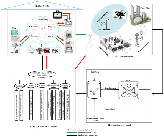
Figure 1.
Proposed modular framework.
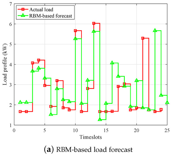
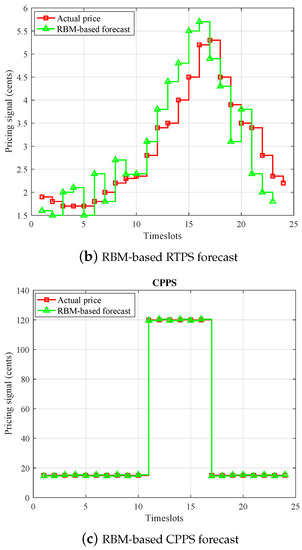
Figure 2.
Price-based DR schemes.
In the proposed modular framework bi-directional communication exists between the power company and residents via AMI. Power company sent price-based DR information to the forecaster module, the forecaster module forecast load and pricing signals of RTPS and CPPS. The HEMC module based on HGWmEDE algorithm receives forecasted results to schedule the household load on the basis of pricing signals such that high power-rating appliances cannot be switched on in peak timeslots. The HEMC module dispatches the load schedule to the power company, and ultimately, the power company sent demanded power of residents. The HEMC can perform the functionalities of logging, management, control, monitoring, and alarm. The purpose is to optimally schedule household load and reduce the frustration of both power company and residents. The profiles of forecasted RTPS and CPPS are illustrated in Figure 2a,b. These two pricing schemes are generated using the data of [37,38].
3.1. Smart Home Appliances Categorization
Smart home appliances are classified into three categories based on operating behavior and energy consumption pattern. The smart home total number of appliances is denoted by a set which includes shiftable appliances, non-shiftable appliances and controllable appliances and is defined by Equation (1).
where denotes shiftable appliances, represents non-shiftable appliances, and denotes controllable appliances. The detailed description of the classification is as follows.
3.1.1. Shiftable Appliances
In shiftable appliances, shifting to any timeslot is allowed, but interruption during operational time is prohibited. Such type of appliances are also known as deferrable appliances. Once operation of such type appliances is started, it cannot be stopped/interrupted until to finish the assigned task [17]. These appliances are the subset of total appliances and are defined by Equation (2).
where WM denotes washing machine, DM represents dishwasher, HS indicates hair straightener, HD denotes hair dryer, MW represents microwave, TP denotes telephone, CP represents computer, OV represents oven, CK denotes cooker, IR represents iron, TR represents toaster, EK, represents electric kettle, and PR represents printer. Each appliance power rating and status at a particular timeslot t is denoted by and , respectively. Equation (3) indicates the ON and OFF status of an appliance.
3.1.2. Controllable Appliances
The controllable appliances have constant operational time and cannot be changed; for example, heating system, lightning, and air conditioning. Such type of appliances are also known as interruptible appliances. The controllable appliances are given by Equation (4).
where represents air conditioner, denotes lighting, and represents heater.
3.1.3. Non-Shiftable Appliances
Non-shiftable appliances are also known as base appliances. Such type of appliances are uncontrollable, and their operational behavior and energy consumption cannot be altered. Televisions and refrigerators are kept in this category due to resembles. The set of non-shiftable appliances is defined by Equation (5).
where TV represents television and RG denotes refrigerator. The overall categorization of smart home appliances is presented in Table 2.
Table 2.
Smart home appliances classification and parameters.
4. Problem Description and Formulation
In DSM, optimal household load scheduling and alignment of residents’ random demand under the generation of the power company is a challenging task. In the literature, various models have been developed to address energy management via the resident load scheduling. For example, the scheduling algorithm is proposed for the energy management of smart homes to reduce the electricity bill, reverse power flow, and peak load shaving [40]. A GWDO algorithm is proposed to schedule the household load under RTPS + IBRS to increase the revenue of residents and reduce the peak to average ratio [41]. Load scheduling is performed using GA under RTPS to alleviate cost and PAR. However, peaks in demand may emerge in OFF-peak hours and user-comfort may compromise while reducing electricity bill because these parameters are conflicting parameters. Thus, a modular framework is proposed, which is based on our proposed algorithm HGWmEDE, for a load scheduling of smart homes with three types of appliances: shiftable appliances, non-shiftable appliances, and controllable appliances, in order to alleviate electricity cost and peaks in demand with affordable appliances waiting time. The purpose is to facilitate both residents and power companies by reducing burden (electricity bill and generation, respectively) on both parties. The peaks in demand reduction are favorable for both residents and power companies because it alleviates the need for peak power plants, which power companies operate when peaks in demand emerged and charged more cost from the residents. To perform effective load scheduling dynamic OTI, RTPS, and CPPS are used. The formulation for energy consumption, cost, peaks in demand, and load scheduling are demonstrated as follows.
4.1. Smart Home Appliances Energy Consumption
The HEMC schedule the smart home appliances under forecasted RTPS and CPPS over a 24-hours time horizon. These smart home appliances when operating according to the schedule consume electrical energy, which can be defined as the electrical energy used by an appliance in unit time and can be measured in the unit. The electrical energy consumed by an appliance can be calculated by Equation (10);
where is the energy consumption of an appliance a at timeslot t, and is the power rating and status of an appliance, respectively. The aggregated electrical energy consumption of the smart home is calculated from the following formula:
where represents the aggregated energy consumption of the smart home appliances.
4.2. Smart Home Appliances Electricity Cost
The electricity cost is defined as the bill deposited by the residents to the power company for the used energy per unit time and per unit price. It is measured in the units of cents. For electricity cost determination, the power company provides various pricing schemes such as RTPS, CPPS, TOUPS, DAPS, and FPS; however, we adopted RTPS and CPPS for the proposed scheme. The RTPS and CPPS are the Midwest independent system operator (MISO) daily electricity pricing schemes taken from federal energy regulatory commission (FERC) [41,42]. The cost for the energy used by the residents under forecasted RTPS and CPPS is as follows:
- electricity cost of resident energy consumption is determined using forecasted RTPS as:where is the total electricity cost by the resident to power company under RTPS denoted by .
- electricity cost paid by the resident to power company under forecasted CPPS is determined as:where is the total electricity cost paid by the resident to power company under CPPS denoted by .
4.3. Peaks in Demand
Peaks in demand is defined as the highest demand emerged over a specified horizon of time such as daily, weekly, monthly, annually, and seasonally, or the highest points of resident electricity consumption. The electric power company cost high from the resident during the peak demand periods because they supplied continues power to load by bringing peak power plants online. It is measure in the units of power (Watts). The proposed framework tries to smooth out the demand curve by reducing the peaks in demand to avoid blackout situation. The peaks in demand can be determined as:
where represents the highest possible peaks in the demand over a specified horizon of time.
4.4. Smart Home Load Scheduling Formulation
The smart home load scheduling problem is formulated as a minimization problem because the main objectives of this work are to alleviate peaks in demand and electricity cost with affordable appliances waiting time.
subjected to:
The constraint (12a) ensures that total energy consumption of residents must be under the capacity of power company. The constraint (12b) and (12c) ensure that the total energy consumption of residents before and after scheduling must be equal subjected to fair comparison. The scheduling of smart appliance is conformed from constraint (12d).
5. Description of Adapted and Proposed Algorithms
In this section, the adapted and proposed heuristic algorithms for smart home load scheduling are discussed. Electricity is consumed in the three demand-side sectors, i.e., residential, commercial, and industrial sectors. However, the main focus is to perform DSM via optimal residential load scheduling. For this purpose, HEMC based on GWO, mEDE, and the proposed HGWmEDE algorithms schedule the smart home appliances to reduce peaks in demand and electricity cost with affordable user discomfort. In the literature, various optimization schemes have been proposed for load scheduling. Some of these techniques outperform in cost reduction and others well perform either in PAR or user-discomfort minimization. In this regard, an optimization technique is proposed, i.e., HGWmEDE, which is a hybrid of mEDE and GWO algorithm. The proposed scheme simultaneously caters the minimization objectives of electricity cost, peaks in demand, and waiting time. The existing and proposed techniques are implemented in MATLAB and their detail description is as follows.
5.1. mEDE
The mEDE is a modified enhanced version of DE. The DE at very first time proposed by Storn in 1995 and enhanced and modified by [43]. It is a meta-heuristic population-based algorithm, which includes four main steps, i.e., population creation, crossover, mutation, and selection [44]. Initially, random population is generated by Equation (13) as follows:
To form a mutant vector, a random function is generated to create three vectors, i.e., , , and . First vector is the target vector and mutant vectors are generated using Equation (14) as given below:
where S is a scaling factor. Mutant vector is generated, then, first three trial vectors are generated by Equations (15)–(17). Then, the best trail vector is selected by comparing with the target vector to update the population with the best trial vectors.
Then, 4th and 5th trial vectors are generated by Equations (18) and (19), respectively, as given below:
The mEDE pseudocode is depicted in Algorithm 1. The maximum iterations are denoted by ; the total population is represented by , it shows the number of possible solutions. The crossover ratio is denoted by , which is taken as 0.30, 0.60, and 0.90. The mutant, trial, and target vectors are represented by m, , and v, respectively.
| Algorithm 1: mEDE |
 |
5.2. GWO
It is a heuristic technique, motivated by the wolves hunting and leadership nature [44]. For leadership 4 levels are defined: , , , and . The is the most intuitive leader among the group, which provides guidance on hunting strategies to other wolves. The and come after in the chronological order, and is the feebler member among the group. Thus, has a lack of leadership qualities and cannot be considered. In HEMC, is taken as the fittest member to schedule the smart home load to reduce cost and peaks in demand. Initially, the population is randomly generated by Equation (20):
where represents the population of gray wolves and is the overall appliances in the smart home, which is used in the proposed framework. The objective function of each search agent can be evaluated using co-efficient D and E.
5.2.1. Encircling Prey
Before hunting the gray wolves encircle a prey. The encircling behavior of gray wolves is mathematically modeled using Equations (21) and (22). These Equations taken from [45].
where the position of prey is represented by , while P is gray wolf position at epoch, which is calculated using Equation (21). The co-efficient vectors D and E are determined according to Equation (23) and Equation (24), respectively:
where and are vectors with random values between 0 and 1. Value of D after multiple epochs is reduced from 2 to 0 while the value of E is randomly taken between 0 and 2. This value of E defines the weight of attractiveness for prey.
5.2.2. Hunting
The provides guidance for hunting, while the , and are secondary participants. The secondary participants follow , due to best knowledge about the prey position. The 3 best solutions are achieved and the other participants such as update its position according to the best solution. The wolves’ position is updated using Equation (25).
where and are determined by Equations (26)–(28).
where and are the best solutions obtained at the iteration; are determined using Equation (23), while are determined using Equations (29)–(31):
where , , and are calculated using Equation (24). The gradation of variable g is conducted in the last step; exploration and exploitation trade-off is controlled by considering value between 0 to 2 in each epoch as depicted in Equation (32).
Mathematical modeling of objective function is shown in Equation (33), which use the power rating and status of an appliance.
From Algorithm 2, the maximum iterations are represented by , the total population is denoted by , the total number of smart home appliances is and is the fitness function. is best among the group participants, which provides a primary optimal solution in the hunting behavior, while and come after in the group and provide secondary optimal solutions.
| Algorithm 2: GWO |
 |
5.3. HGWmEDE
In this section, the proposed hybrid algorithm is demonstrated in detail. Initial population in mEDE is generated by four phases, i.e., initialization phase, mutation phase, crossover phase, and selection phase and the population are updated by comparatively analyzing trial vector with the target vector. The procedure of trail vector selection is effective in choosing the best trial vector from available vectors. The GWO comprised of three steps, i.e., encircling prey, hunting, and wolves position update within the pack. All search agents’ positions are updated according to the leader within the pack. In GWO, unlike the mEDE agents, with , and are not compared. However, the and are closer to the prey as compared to . To conduct a comparison of all search agents a crossover phase of mEDE is adopted. Thus, the best search agent is selected according to the crossover phase of mEDE and search agents’ position is updated according to GWO. The HGWmEDE is proposed by combining the taking key characteristics of both mEDE and GWO.
In Algorithm 3, the detailed stepwise procedure of HGWmEDE is presented. The main stages of the proposed HGWmEDE algorithm are initialization stage, encircling prey stage, best search agent selection stage, and wolves position update stage. Initially, the population of wolves is generated randomly using Equation (20). The best search agent is selected by following the steps presented in Algorithm. The mutant vector m is generated using Equation (14). The fitness of m, , and is computed by Equation (33). Crossover phase is conducted to select the best search agent using the following Equations:
| Algorithm 3:HGWmEDE |
 |
When the best search agents are selected then search agents’ position is updated according to GWO. The position is updated using Equation (25).
The detail description of Algorithm 3 for each step is as follows. In 1st step, parameters are initialized. In 2nd step, randomly population is generated, and the counter is adjusted to maximum epochs. Crossover phase of mEDE is conducted to compare the fitness of the mutant vector with , , and . The search agent status is updated using GWO. The procedure is repeated for several epochs until the termination criteria are reached.
6. Simulation Results and Discussion
Simulation results and discussions of the proposed modular framework are demonstrated, in this section. The pricing signals used for load scheduling is forecasted using RBM. The aim is to evaluate the performance (peaks in demand and electricity cost reduction) of proposed and existing schemes under RBM-based forecasted RTPS and CPPS for different OTI. The HEMC is responsible for scheduling the appliances using the forecasted RTPS and CPPS pricing signals. The performance is evaluated for different OTI such as 15, 30, and 60 timeslots. The home appliances and their parameters such as OTI, LOT, starting time, ending time, and power rating are adopted from [39]. Simulation results and discussion of the proposed and existing algorithms are demonstrated in the succeeding sections in terms of peaks in the demand and electricity cost reduction with affordable appliances waiting time. The detail description is as follows.
6.1. Electricity Cost Evaluation under Price-Based DR
The power company provides various pricing schemes such as RTPS, CPPS, TOUPS, DAPS, and FPS for electricity cost calculation; however, we adopted RTPS and CPPS for the proposed framework. The RTPS and CPPS are the Midwest independent system operator (MISO) daily electricity pricing signals taken from the federal energy regulatory commission (FERC). The electricity cost using RTPS and CPPS is individually discussed in the succeeding sections.
6.2. Electricity Cost Evaluation Using RTPS
To evaluate the cost parameters of the proposed scheme simulations are conducted using different OTI, i.e., 15, 30, and 60 min. The proposed HGWmEDE algorithm reduced electricity cost as compared to GWO and mEDE by scheduling smart home appliances using forecasted RTPS. The scheduled appliances sustain coordination among pricing scheme and the consumption pattern in a particular timeslot of a day to alleviate the electricity cost. The proposed algorithm shifts smart home appliances from ON-peak timeslots to OFF-peak timeslots in an optimal manner to alleviate electricity cost and peaks in demand.
The energy consumption pattern in terms of electricity cost of the proposed and existing algorithms with 15 min OTI is illustrated in Figure 3a. In this Figure 3a, both scheduled and unscheduled scenarios are observed. The peaks in demand are high in case of unscheduled load, which reveals that prices are high in these particular hours. Thus, the use of appliances in these hours results in high electricity cost. However, scheduling smart home appliances using the proposed and existing algorithms eliminate these peaks in demand and reduce the electricity cost. Thus, the proposed HGWmEDE-based framework outperforms both GWO and mEDE in terms of peaks in demand and electricity cost reduction. The electricity cost pattern of the proposed and existing algorithms with 30 min OTI under RTPS is illustrated in Figure 3b. Both proposed and existing algorithms-based HEMC can schedule smart home appliances. However, the electricity cost of GWO is high at the starting timeslots, while HGWmEDE has minimum electricity cost throughout the 24 h. Likewise, in Figure 3c, the electricity cost pattern of the proposed and existing algorithms for 60 min OTI under RTPS is depicted. The proposed HGWmEDE algorithm has reduced the electricity cost by optimally scheduling smart home appliances of resident’s, which is one of our main objectives.
Figure 3.
Electricity cost per timeslot evaluation for different OTI under RTPS.
The Figure 4 illustrate that the proposed framework optimally scheduled the smart home appliances as compared to mEDE and GWO under forecasted RTPS and CPPS and reduced the overall aggregated electricity cost of the residents.
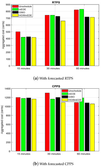
Figure 4.
Aggregated electricity cost evaluation under forecasted RTPS and CPPS.
Figure 4a presents the overall electricity bill of 15, 30, and 60 OTI under forecasted RTPS. The electricity cost of unscheduled load for 15 min OTI is measured as 500.4827 cents. However, with scheduling smart home appliances using mEDE and GWO reduced the overall electricity cost to 420.5381 cents and 426.0508 cents, respectively. The proposed HGWmEDE scheme reduced electricity cost up to 416.7468 cents, which is the maximum reduction as compared to mEDE and GWO. In a similar fashion, electricity cost reduction behavior of the proposed and existing schemes can be observed for both 30 and 60 min OTI.
Electricity Cost Evaluation under CPPS for Different OTI
The load scheduling is favorable for both residents and power company because it reduces electricity cost, which is favorable for residents; and peaks in the demand, which is favorable for the power company. Cost reduction facilitates residents to deposit less electricity bill and peaks reduction in the demand facilitate power company in the optimal management of supply with demand. In this subsection, electricity cost evaluation is conducted under the forecasted CPPS profile. The electricity bill reduction evaluation of the proposed and existing algorithms are performed using 15, 30, and 60 min OTI under CPPS and is illustrated in Figure 5. The electricity cost profile of 15 min OTI is depicted in Figure 5a. Generally, the forecasted CPPS remains constant except during critical peak hours where the electricity price reaches to its maximum value [46]. The timeslots from 40 to 65 are critical periods, where the electricity price is high. In unscheduled load scenario, the maximum peak is at 181.55 cents. The scheduled load scenario, where smart home appliances are scheduled, and the peak is reduced to 83.07 cents. The electricity cost for 30 min OTI is illustrated in Figure 5b. The electricity cost is varying for 48 timeslots and the remaining electricity cost profile is as the same as observed in Figure 5a. In our proposed HGWmEDE algorithm-based scenario, no peaks in demand are emerged except at the starting time of day, which is 56 cents. The electricity cost for 60 min OTI is depicted in Figure 5c. The unscheduled appliance electricity cost reaches to 766.8 cents, which is reduced to 203.46 cents when these smart home appliances are scheduled using our proposed HGWmEDE algorithm. This means that the proposed HGWmEDE algorithm optimally scheduled the smart home appliances. The overall cost for the proposed and existing optimization schemes is illustrated in Figure 4b. The overall unscheduled cost is 1300.891 cents, which is reduced to 1085.91 cents when smart home appliances are scheduled using the proposed HGWmEDE algorithm. The proposed HGWmEDE algorithm outperforms both mEDE and GWO algorithms in terms of electricity cost reduction. The overall electricity cost reduction for 30 and 60 min OTI is depicted in Figure 4b. A brief comparison of electricity cost under forecasted RTPS and CPPS is listed in Table 3 for 15, 30, and 60 min OTI.
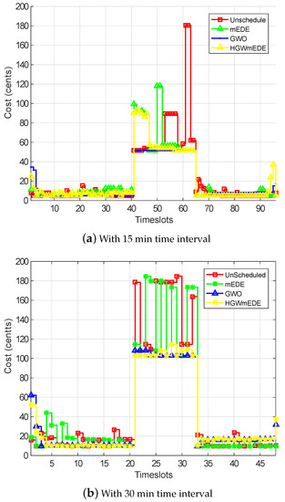
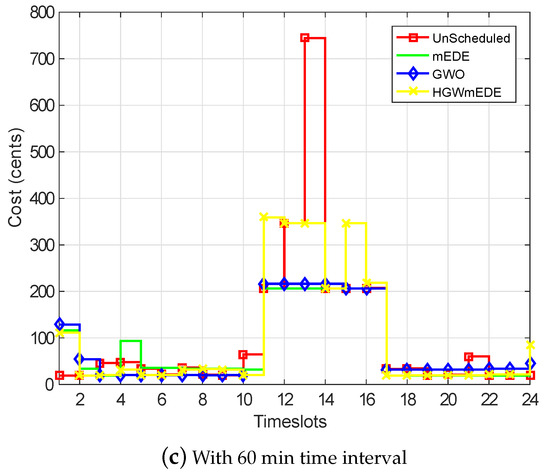
Figure 5.
Electricity cost per timeslot evaluation under forecasted CPPS for different OTI.
Table 3.
Overall electricity cost comparative evaluation for 24 h time horizon under forecasted RTPS and CPPS.
6.3. Smart Home Energy Consumption
The smart home appliances energy consumption for both RTPS and CPPS are discussed in detail in the following subsection:
6.3.1. Smart Home Energy Consumption Using RTPS
Energy consumed by smart home appliances under RTPS in each timeslot for 15, 30, and 60 min OTIs is illustrated in Figure 6. In Figure 6a, the smart home energy consumption profile for 15 min OTI is depicted. From the figure it is obvious that at the start and end timeslots of the day have low per unit electricity price; Thus, HEMC based on our proposed HGWmEWDE shifted the load to these low pricing timeslots. In this manner, the proposed scheme optimally curtailed peak load on the power company.
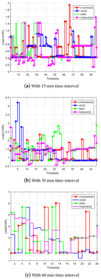
Figure 6.
Electricity energy consumption evaluation per timeslot under forecasted RTPS.
The smart home energy consumption profile for 30 min time interval is illustrated in Figure 6b. The HMEC based on our proposed HGWDE algorithm results in optimal energy consumption profile as compared to GWO and mEDE-based HEMC. The HGWmEDE eliminated load peaks, which curtailed burden on both power company in terms of peak power generation and on residents in terms reduce electricity bill deposit. The mEDE and GWO also reduced peaks in demand and reduced the burden on both power company and residents as compared to without scheduling scenario. The burden reduction of the proposed scheme is more as compared to the existing schemes (GWO and mEDE); thus, the proposed scheme outperforms the existing schemes.
In Figure 6c, energy consumption pattern for 60 min OTI is depicted. The electricity prices are low during starting timeslots and ending timeslots in forecasted RTPS profile. Thus, the proposed and existing schemes shifted most of the load to these low-price timeslots. The prices are maximum from 3 to 7 p.m., so, our proposed scheme not scheduled appliance in these timeslots because the operation of appliances during these timeslots results in high electricity cost. Load shifting from ON-peak timeslots to OFF-peak timeslots results in user discomfort as the residents must stay to switch on a particular smart home appliance because of the trade-off between electricity cost and user-comfort.
The smart home overall energy consumption for 15 min OTI is 56.3108 kWh, which remains the same before and after scheduling subjected to a fair comparison. The scheduled and unscheduled energy consumption for 30 min OTI is same and recorded as 57.7656 kWh. Likewise, for 60 min OTI, smart home overall energy consumption for both scheduled and unscheduled scenarios is the same and recorded as 64.5661 kWh.
6.3.2. Energy Consumption Using CPPS
In this subsection, the proposed HGWmEDE scheme is comparatively evaluated under forecasted CPPS for 15, 30, and 60 min OTI. The comparison is illustrated in Figure 7. The smart home energy consumption profile for 96 timeslots is depicted in Figure 7a. The proposed scheme shifted load to the timeslots where electricity price is low to reduce cost and peaks in demand. In CPPS, at starting and ending timeslots electricity price is constant, while during 40 to 65 timeslots price is maximum as illustrated in Figure 2b. The profile GWO and HGWmEDE is almost similar, except some peaks of GWO are much higher than HGWmEDE at starting timeslots. The proposed HGWmEDE eliminates the peaks in demand for 30 min OTI case; however, the existing schemes have high peaks as compared to the proposed HGWmEDE scheme.
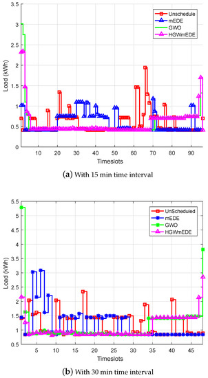
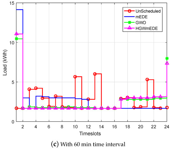
Figure 7.
Smart home energy consumption per timeslot evaluation using CPPS.Optional caption for list of Figure 5-8
The energy consumption for 60 min OTI is illustrated in Figure 7c. The energy consumption for all cases remain same but the status of appliances vary according to the schedule of HEMC based on our proposed HGWmEDE algorithm and existing algorithm.
The overall energy consumption with and without scheduling must remain same subjected to a fair comparison. The overall energy consumption for 15 min OTI is 56.3107 kWh for the proposed (HGWmEDE) and existing (GWO and mEDE) schemes. Similarly, the energy consumption for 30, and 60 min OTI are 57.7656 kWh and 64.5661 kWh, respectively. Thus, both electricity cost and peaks in demand are reduced by scheduling the smart home appliance while keeping the energy consumption constant.
6.4. Peaks in Demand
Peaks in demand are defined as the value of peak load emerged during a time horizon of 24 h or the maximum load switched on by user during 24 h time horizon. Our objective is to reduce the peaks in demand and to ensure smooth demand curve for 24 h time horizon. Various DSM programs can be applied to alleviate peaks in demand such as peak clipping, load shifting, and price-based DR to eliminate peaks in demand and smooth the demand curve. Peaks elimination in the demand reduces the electricity cost and burden on the power company. The peaks reduction in demand is evaluated for both RTPS and CPPS in the succeeding section.
6.4.1. Peaks Reduction in Demand Evaluation under RTPS
The peaks reduction in demand evaluation under RTPS for different OTI is depicted in Figure 8a. In case, when the load is not scheduled the peak emerged in demand is 10.9697. In case, when the load is scheduled based on mEDE and GWO, the peaks emerged in demand are 8.1722 and 5.6750, respectively. The peak emerged for proposed HGWmEDE scheme is 5.1530, which is low as compared to the both unscheduled and scheduled (GWO and mEDE) cases. The percentage reduction in peaks of the proposed HGWmEDE scheme is 53.02%, while the percentage reduction in peaks of the GWO and mEDE is 25.50%, 48.26%, respectively. Thus, the proposed HGWmEDE scheme outperforms the other schemes in terms of peaks reduction in demand.
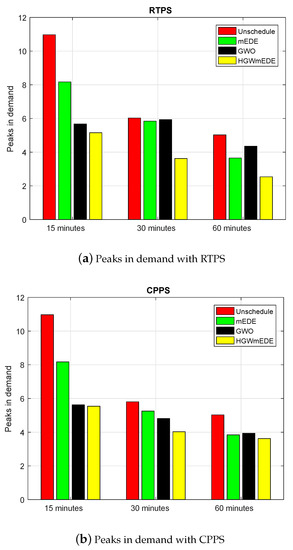
Figure 8.
Peaks in demand evaluation under forecasted RTPS and CPPS for different OTI.
In case of unscheduled load for 30 min OTI, the peak emerged in demand is recorded as 6.0257; however, the peak has reduced to 5.8424 and 5.9335 when the load is scheduled using mEDE and GWO algorithms. The proposed HGWmEDE scheme outperforms both mEDE and GWO schemes by reducing peak in demand to 3.6209. Similarly, for 60 min OTI, mEDE, GWO, and HGWmEDE reduced the peaks in demand by a value of 3.6559, 4.3510 and 2.5370 as compared to without scheduling case, which is 5.0245. Thus, it is obvious from the aforementioned statistical analysis that the proposed HGWmEDE scheme outperforms both mEDE and GWO schemes.
6.4.2. Peaks in Demand Evaluation under CPPS for Different OTI
Evaluation of peaks in demand under CPPS is illustrated in Figure 8b. In case of unscheduled load for 15 min OTI, peak in demand is recorded as 10.9697. However, after performing load scheduling, peak in demand is alleviated to 5.5416 with HGWmEDE, 5.627 with GWO and 8.1723 with mEDE. Peaks reduction in terms of percentage for the proposed HGWmEDE, mEDE, GWO, are 49.4836%, 48.7120%, and 25.5012%, respectively.
In case of unscheduled load for 30 min OTI, the peak emerged is 5.86. After load scheduling with mEDE, GWO, and HGWmEDE, peaks in demand are recorded as 5.2536, 4.8165, and 4.0215, respectively. Thus, the proposed HGWmEDE scheme outperforms the existing (mEDE and GWO) schemes in terms of peaks reduction in demand. The comparative evaluation of the proposed HGWmEDE and existing (mEDE and GWO) schemes in terms of peaks reduction in demand under RTPS and CPPS for different OTI is listed in Table 4.
Table 4.
Peaks in demand evaluation of the proposed and existing schemes for 24 h.
6.5. User-Comfort Evaluation in Terms of Waiting Time
In this subsection, the user-comfort in terms of waiting time is evaluated. In nature, always there is a trade-off between different conflicting parameters. In this paper, a trade-off between electricity cost and waiting time (user-comfort) exist. To reduce electricity cost, the residents must wait for timeslots where the electricity price is low, i.e., OFF-peak hours to switch on their load. Thus, user-comfort and electricity cost are directly related to [47]. In without scheduling scenario, waiting time is almost zero because the smart home appliances are operated according to the resident choice and priority. However, the case when the load is scheduled based on mEDE, GWO, and the proposed HGWmEDE, the user switched on their appliances according to the schedule provided by HEMC to reduce electricity cost. Thus, user-comfort is compromised while reducing the electricity cost due to the trade-off. Evaluation of appliances waiting time under RTPS and CPPS are as follows:
6.5.1. Smart Home Appliances Waiting Time Evaluation under RTPS
The appliance waiting time for 15, 30, and 60 min OTI is illustrated in Figure 9a. Waiting time of the proposed HGWmEDE, mEDE, and GWO for 15 min OTI are calculated as 10.4 h, 4.3 h, and 9.7 h, respectively. Waiting time for 30 min OTI of the proposed HGWmEDE, mEDE, and GWO are calculated as 12.7007 h, 4.5394 h, and 10.0262 h. Similarly, for 60 min OTI of the proposed HGWmEDE, mEDE, and GWO, waiting time is 3.8 h, 2.6560 h, and 2.2397 h, respectively.
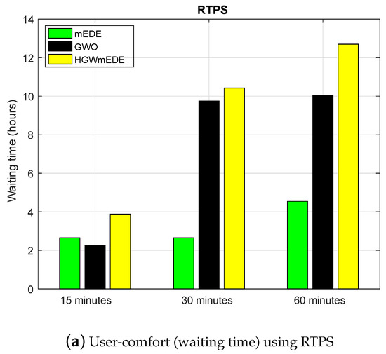
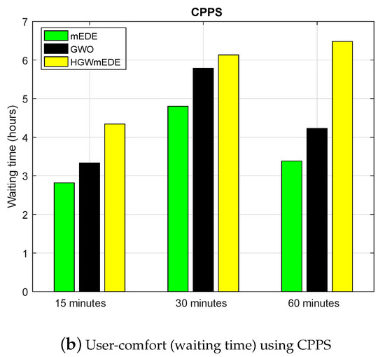
Figure 9.
User-comfort (waiting time) of the scheduled load based on the proposed HGWmEDE, mEDE, and GWO using RTPS and CPPS.
It is concluded from the above results and discussion that user frustration in terms of waiting time always reduces by keeping the OTI smaller. For example, for 15 min OTI, if the operational time of a toaster is 12 min, then HEMC will allocate 15 min timeslot to toaster; in this way, only 3 min of a timeslot is wasted because this slot is not allocated to other appliances. In contrast, in case of 60 min OTI, the HEMC will allocate 60 min timeslot to an electric kettle, which has the operational time of only 5 min, then rest of 55 min timeslots will be wasted. Thus, in larger OTI, the user frustration increase in terms of waiting time.
6.5.2. Smart Home Appliances Waiting Time Evaluation under CPPS
Waiting time of the proposed HGWmEDE and existing (mEDE and GWO) under CPPS is illustrated in Figure 9b. The recorded value of waiting time for mEDE, GWO, and the proposed HGWmEDE is as 3.39 h, 4.23 h, and 6.49 h, respectively. It is obvious that the load schedule return by HMEC based on HGWmEDE algorithm has more waiting time, which indicates that user-comfort is compromised for the purpose to reduce electricity cost. The statistical analysis of the proposed and existing algorithms in terms of waiting time for different OTI under RTPS and CPPS is listed in Table 5.
Table 5.
Comparative evaluation of the proposed HGWmEDE and existing (mEDE and GWO) algorithm in terms of waiting time under RTPS and CPPS for different OTI.
6.6. Convergence Evaluation of the Proposed HGWmEDE Algorithm-Based Fitness Function
The convergence evaluation of the fitness function of the proposed HGWDE algorithm is depicted in Figure 10. X-label of the plot is the number of iterations and Y-label is the value of the fitness function. Figure 10 illustrates that the solution converges after 100 iterations, which indicates that the global maximum is achieved. The proposed HGWmEDE algorithm converging behavior for each iteration is plotted. The value of cost is constantly decreasing from 0 to 10 iterations and after these iterations, the graph slight varies. The behavior of convergence of the proposed HGWDE algorithm iterations is observed for 100 iterations. Finally, a straight line is achieved, which means that the solution is converged, and this is the most optimal point.
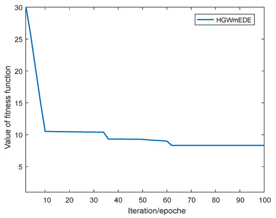
Figure 10.
Convergence evaluation of the fitness function.
6.7. Performance Trade-Off
The performance trade-off exists in various conflicting parameters of the system. In the proposed modular framework, a trade-off between electricity cost and user-comfort exist. When the residents wants to reduce their electricity cost, he must face frustration in the form of user discomfort. Residents frustration increasing when the difference between the resident preferred time and the HEMC scheduled time is more. It is observed in Figure 4a,b that the electricity cost is reduced by applying HGWmEDE for scheduling at the expense of maximum average waiting time.
7. Conclusions and Future Research Directions
In this paper, first a modular framework is introduced, and then an algorithm HGWmEDE is proposed, which with the help of forecasted price-incentive DR scheme schedule the household load to maximize the aggregate utility of both resident and power company. The proposed approach is beneficial for residents because it reduces the electricity bill with an affordable waiting time of smart home appliances. In addition, it is beneficial for the power company because it reduces peaks in demand, which smooth out the demand curve and increase the stability of the power system. The integration of the forecaster module to the home energy management framework provides optimal load schedule, which not only facilitates residents but also power companies. Simulation analysis validated the proposed approach by comparing with two other approaches, a system without HEMC and a system with HEMC based on GWO and mEDE algorithms. Surely, the proposed framework can be applied for DSM and reliable operation of the SG. The idea of this paper in the future can be extended to various directions:
- A system with renewable and non-renewable energy provider can be considered.
- A system with a deep neural network can be used to optimize home energy management.
- A system with multiple power companies and multiple homes and effect malicious residents can be considered.
- To implement fog and cloud concept for household load scheduling instead of using a HEMC.
- The same framework can be extended for other heuristics, deterministic, and stochastic techniques under RES.
Author Contributions
Conceptualization, G.H.; Formal analysis, S.A. and M.U.; Investigation, G.H.; Methodology, G.H. and K.S.A.; Software, G.H.; Supervision, K.S.A.; Validation, K.S.A., N.I. and A.A.; Writing—original draft, G.H.; Writing—review and editing, K.S.A., S.A., and M.U.
Funding
This research received no external funding.
Conflicts of Interest
The authors declare no conflicts of interest.
Nomenclature
| Acronym | Meaning |
| RTPS | Real-Time Pricing Scheme |
| TOUPS | Time of Use Pricing Scheme |
| CPPS | Critical Peak Pricing Scheme |
| FRPS | Flat-Rate Pricing Scheme |
| DAPS | Day-Ahead Pricing Scheme |
| HEMC | HEM controller |
| DSM | Demand-Side Management |
| HGWmEDE | Hybrid Gray Wolf-Modified Differential Evolution |
| RBM | Restricted Boltzmann Machine |
| LOT | Length of Operational Time |
| OTI | Operation Time Interval |
| GA | Genetic Algorithm |
| BPSOA | Binary-Particle Swarm Optimization Algorithm |
| DEA | Differential Evolution Algorithm |
| IDSS | Intelligent Decision Support System |
| WDO | Wind-Driven Optimization |
| K-WDO | Algorithm with Knapsack |
| ACOA | Ant Colony Optimization Algorithm |
| MOEA | Multi-Objective Evolutionary Algorithm |
| PS | Pareto Sets |
| GMI | Generalized Mutual Information |
| TLBOA | Teaching and Learning-Based Optimization Algorithm |
| SFL | Shuffled-Frog Leaping |
| ANN-GA | Artificial Neural Network |
| LP | Linear Programming |
| NLP | Non-LP |
| BFA | Bacterial Foraging Algorithm |
| DR | Demand Response |
| AMI | Advanced Metering Infrastructure |
| ICT | Information and Communication Technology |
| RERs | Renewable Energy Resources |
| SG | Smart Grid |
References
- Mhanna, S.; Chapman, A.C.; Verbi, G. A fast distributed algorithm for large-scale demand response aggregation. IEEE Trans. Smart Grid 2016, 7, 2094–2107. [Google Scholar] [CrossRef]
- Energy Reports. Available online: http://www.enerdata.net/enerdatauk/press-and-publication/ energy-features/enerfuture-2007.php (accessed on 10 January 2019).
- Logenthiran, T.; Srinivasan, D.; Shun, T.Z. Demand side management in smart grid using heuristic optimization. IEEE Trans. Smart Grid 2012, 3, 1244–1252. [Google Scholar] [CrossRef]
- Shirazi, E.; Jadid, S. Optimal residential appliance scheduling under dynamic pricing scheme via HEMDAS. Energy Build. 2015, 93, 40–49. [Google Scholar] [CrossRef]
- Bradac, Z.; Kaczmarczyk, V.; Fiedler, P. Optimal scheduling of domestic appliances via MILP. Energies 2014, 8, 217–232. [Google Scholar] [CrossRef]
- Katz, J.; Andersen, F.M.; Morthorst, P.E. Load-shift incentives for household demand response: Evaluation of hourly dynamic pricing and rebate schemes in a wind-based electricity system. Energy 2016, 115, 1602–1616. [Google Scholar] [CrossRef]
- Rabiya, K.; Javaid, N.; Rahim, M.H.; Aslam, S.; Sher, A. Fuzzy energy management controller and scheduler for smart homes. Sustain. Compu. Inf. Syst. 2019, 21, 103–118. [Google Scholar]
- Adika, O.C.; Wang, L. Autonomous appliance scheduling for household energy management. IEEE Trans. Smart Grid 2014, 5, 673–682. [Google Scholar] [CrossRef]
- Li, C.; Yu, X.; Yu, W.; Chen, G.; Wang, J. Efficient computation for sparse load shifting in demand side management. IEEE Trans. Smart Grid 2017, 8, 250–261. [Google Scholar] [CrossRef]
- Javaid, N.; Naseem, M.; Rasheed, M.B.; Mahmood, D.; Khan, S.A.; Alrajeh, N.; Iqbal, Z. A new heuristically optimized Home Energy Management controller for smart grid. Sustain. Cities Soc. 2017, 34, 211–227. [Google Scholar] [CrossRef]
- Bilal, H.; Javaid, N.; Hasan, Q.; Javaid, S.; Khan, A.; Malik, S. An inventive method for eco-efficient operation of home energy management systems. Energies 2018, 11, 3091. [Google Scholar]
- Huang, Y.; Wang, L.; Guo, W.; Kang, Q.; Wu, Q. Chance constrained optimization in a home energy management system. IEEE Trans. Smart Grid 2018, 9, 252–260. [Google Scholar] [CrossRef]
- Ogwumike, C.; Short, M.; Abugchem, F. Heuristic Optimization of Consumer Electricity Costs using a Generic Cost Model. Energies 2016, 9, 6. [Google Scholar] [CrossRef]
- Rasheed, M.B.; Javaid, N.; Ahmad, A.; Khan, Z.A.; Qasim, U.; Alrajeh, N. An efficient power scheduling scheme for residential load management in smart homes. Appl. Sci. 2015, 5, 1134–1163. [Google Scholar] [CrossRef]
- Tuaimah, F.M.; Abd, Y.N.; Hameed, F.A. Ant Colony Optimization based Optimal Power Flow Analysis for the Iraqi Super High Voltage Grid. Int. J. Comput. Appl. 2013, 67, 13–18. [Google Scholar]
- Logenthiran, T.; Srinivasan, D.; Vanessa, K.W.M. Demand side management of smart grid: Load shifting and incentives. J. Renew. Sustain. Energy 2014, 6, 033136. [Google Scholar] [CrossRef]
- Islam, S.M.; Das, S.; Ghosh, S.; Roy, S.; Suganthan, P.N. An adaptive differential evolution algorithm with novel mutation and crossover strategies for global numerical optimization. IEEE Trans. Syst. Man Cybern. Part B 2012, 42, 482–500. [Google Scholar] [CrossRef] [PubMed]
- Li, H.; Zhang, Q. Multiobjective optimization problems with complicated Pareto sets, MOEA/D and NSGA-II. IEEE Trans. Evol. Comput. 2009, 13, 284–302. [Google Scholar] [CrossRef]
- Setlhaolo, D.; Xia, X. Optimal scheduling of household appliances incorporating appliance coordination. Energy Proc. 2014, 61, 198–202. [Google Scholar] [CrossRef]
- Osório, G.J.; Matias, J.C.O.; Catalão, J.P.S. Electricity prices forecasting by a hybrid evolutionary-adaptive methodology. Energy Convers. Manag. 2014, 80, 363–373. [Google Scholar] [CrossRef]
- Shayeghi, H.; Ghasemi, A.; Moradzadeh, M.; Nooshyar, M. Simultaneous day-ahead forecasting of electricity price and load in smart grids. Energy Convers. Manag. 2015, 95, 371–384. [Google Scholar] [CrossRef]
- Derakhshan, G.; Shayanfar, H.A.; Kazemi, A. The optimization of demand response programs in smart grids. Energy Policy 2016, 94, 295–306. [Google Scholar] [CrossRef]
- Soares, J.; Ghazvini, M.A.F.; Vale, Z.; de Moura Oliveira, P.B. A multi-objective model for the day-ahead energy resource scheduling of a smart grid with high penetration of sensitive loads. Appl. Energy 2016, 162, 1074–1088. [Google Scholar] [CrossRef]
- Ghasemi, A.; Shayeghi, H.; Moradzadeh, M.; Nooshyar, M. A Novel hybrid algorithm for electricity price and load forecasting in smart grids with demand-side management. Appl. Energy 2016, 177, 40–59. [Google Scholar] [CrossRef]
- Jayabarathi, T.; Raghunathan, T.; Adarsh, B.R.; Suganthan, P.N. Economic dispatch using hybrid grey wolf optimizer. Energy 2016, 111, 630–641. [Google Scholar] [CrossRef]
- Asif, K.; Javaid, N.; Khan, M.I. Time and device based priority induced comfort management in smart home within the consumer budget limitation. Sustain. Cities Soc. 2018, 41, 538–555. [Google Scholar]
- Geem, Z.W.; Kim, J.H.; Loganathan, G.V. A new heuristic optimization algorithm: Harmony 578 search. Simulation 2001, 76, 60–68. [Google Scholar] [CrossRef]
- Storn, R.; Price, K. Differential Evolution—A Simple and Efficient Adaptive Scheme for Global 580 Optimization over Continuous Spaces; International Computer Science Institute: Berkeley, CA, USA, 1995. [Google Scholar]
- Vardakas, J.S.; Zorba, N.; Verikoukis, C.V. Performance evaluation of power demand scheduling scenarios in a smart grid environment. Appl. Energy 2015, 142, 164–178. [Google Scholar] [CrossRef]
- Awais, M.; Javaid, N.; Ullah, I.; Abdul, W.; Almogren, A.; Alamri, A. An intelligent hybrid heuristic scheme for smart metering based demand side management in smart homes. Energies 2017, 10, 1258. [Google Scholar]
- Yuce, B.; Rezgui, Y.; Mourshed, M. ANN–GA smart appliance scheduling for optimised energy management in the domestic sector. Energy Build. 2016, 111, 311–325. [Google Scholar] [CrossRef]
- Reka, S.S.; Ramesh, V. A demand response modeling for residential consumers in smart grid environment using game theory based energy scheduling algorithm. Ain Shams Eng. J. 2016, 7, 835–845. [Google Scholar] [CrossRef]
- Erdinc, O. Economic impacts of small-scale own generating and storage units, and electric vehicles under different demand response strategies for smart households. Appl. Energy 2014, 126, 142–150. [Google Scholar] [CrossRef]
- Agnetis, A.; de Pascale, G.; Detti, P.; Vicino, A. Load scheduling for household energy consumption optimization. IEEE Trans. Smart Grid 2013, 4, 2364–2373. [Google Scholar] [CrossRef]
- Setlhaolo, D.; Xia, X.; Zhang, J. Optimal scheduling of household appliances for demand response. Electr. Power Syst. Res. 2014, 116, 24–28. [Google Scholar] [CrossRef]
- Pradhan, M.; Roy, P.K.; Pal, T. Grey wolf optimization applied to economic load dispatch problems. Int. J. Electr. Power Energy Syst. 2016, 83, 325–334. [Google Scholar] [CrossRef]
- Vardakas, J.S.; Zorba, N.; Verikoukis, C.V. Power demand control scenarios for smart grid applications with finite number of appliances. Appl. Energy 2016, 162, 83–98. [Google Scholar] [CrossRef]
- Ogunjuyigbe, A.S.O.; Ayodele, T.R.; Akinola, O.A. User satisfaction-induced demand side load management in residential buildings with user budget constraint. Appl. Energy 2017, 187, 352–366. [Google Scholar] [CrossRef]
- Javaid, N.; Ullah, I.; Akbar, M.; Iqbal, Z.; Khan, F.A.; Alrajeh, N.; Alabed, M.S. An intelligent load management system with renewable energy integration for smart homes. IEEE Access 2017, 5, 13587–13600. [Google Scholar] [CrossRef]
- Yao, E.; Samadi, P.; Wong, V.W.S.; Schober, R. Residential demand side management under high penetration of rooftop photovoltaic units. IEEE Trans. Smart Grid 2016, 7, 1597–1608. [Google Scholar] [CrossRef]
- Nadeem, J.; Hafeez, G.; Iqbal, S.; Alrajeh, N.; Alabed, M.S.; Guizani, M. Energy efficient integration of renewable energy sources in the smart grid for demand side management. IEEE Access 2018, 6, 77077–77096. [Google Scholar]
- Ghulam, H.; Javaid, N.; Iqbal, S.; Khan, F. Optimal residential load scheduling under utility and rooftop photovoltaic units. Energies 2018, 11, 611. [Google Scholar]
- Ashfaq, A.; Javaid, N.; Guizani, M.; Alrajeh, N.; Khan, Z.A. An accurate and fast converging short-term load forecasting model for industrial applications in a smart grid. IEEE Trans. Ind. Inform. 2017, 13, 2587–2596. [Google Scholar]
- Muqaddas, N.; Iqbal, Z.; Javaid, N.; Khan, Z.; Abdul, W.; Almogren, A.; Alamri, A. Efficient power scheduling in smart homes using hybrid grey wolf differential evolution optimization technique with real time and critical peak pricing schemes. Energies 2018, 11, 384. [Google Scholar]
- Singh, N.; Singh, S.B. Hybrid Algorithm of Particle Swarm Optimization and Grey Wolf Optimizer for Improving Convergence Performance. J. Appl. Math. 2017, 2017, 2030489. [Google Scholar] [CrossRef]
- Waterloo North Hydro. Available online: https://www.wnhydro.com/en/your-home/time-of-use-rates.asp (accessed on 9 January 2019).
- Muralitharan, K.; Sakthivel, R.; Shi, Y. Multiobjective optimization technique for demand side management with load balancing approach in smart grid. Neurocomputing 2016, 177, 110–119. [Google Scholar] [CrossRef]
© 2019 by the authors. Licensee MDPI, Basel, Switzerland. This article is an open access article distributed under the terms and conditions of the Creative Commons Attribution (CC BY) license (http://creativecommons.org/licenses/by/4.0/).