Numerical and Analytical Investigation of an Unsteady Thin Film Nanofluid Flow over an Angular Surface
 ,
,  , ,
, ,
Abstract
1. Introduction
2. Problem Formulation
3. Solution Methodology
4. Results and Discussion
5. Conclusions
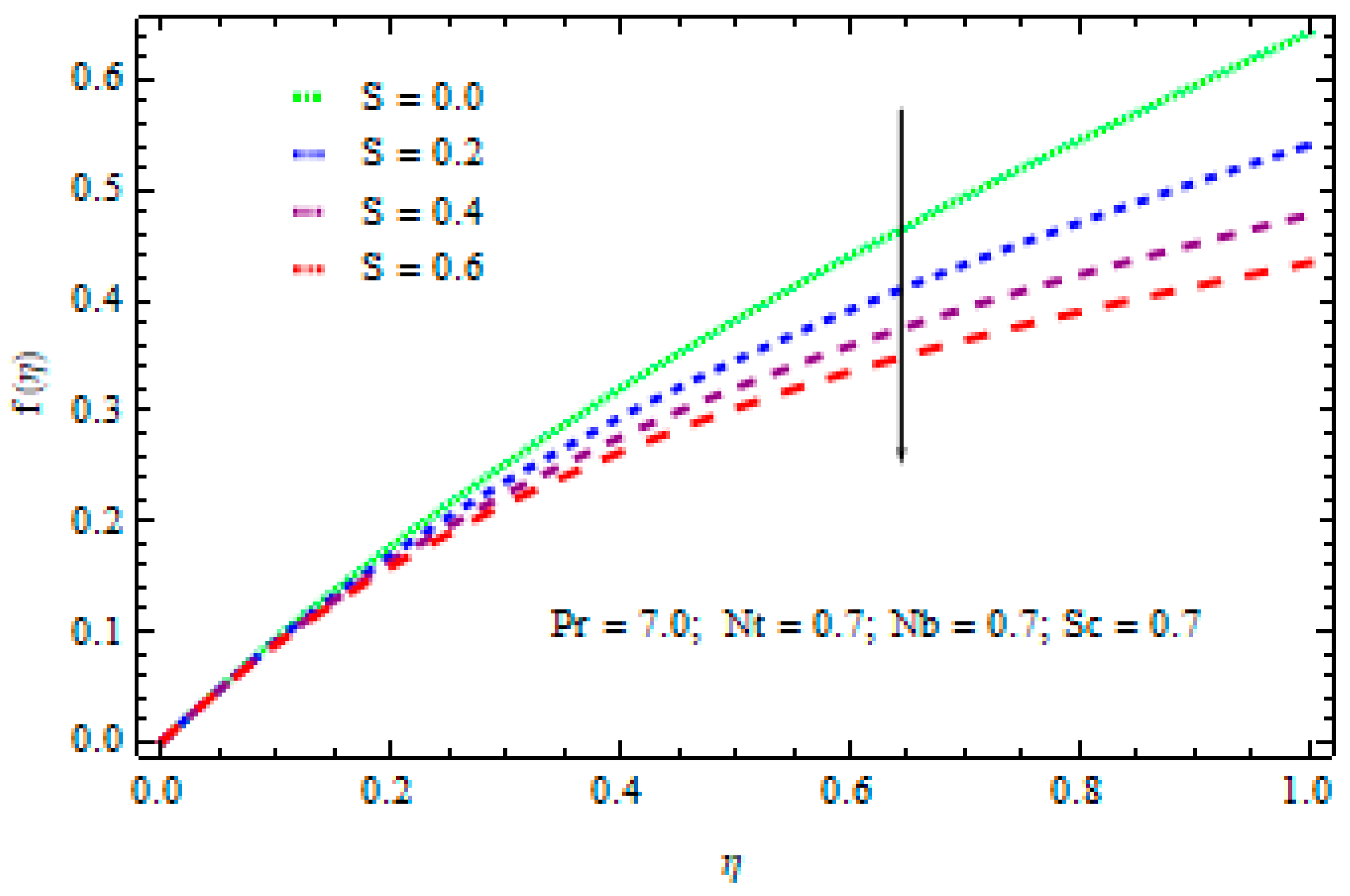
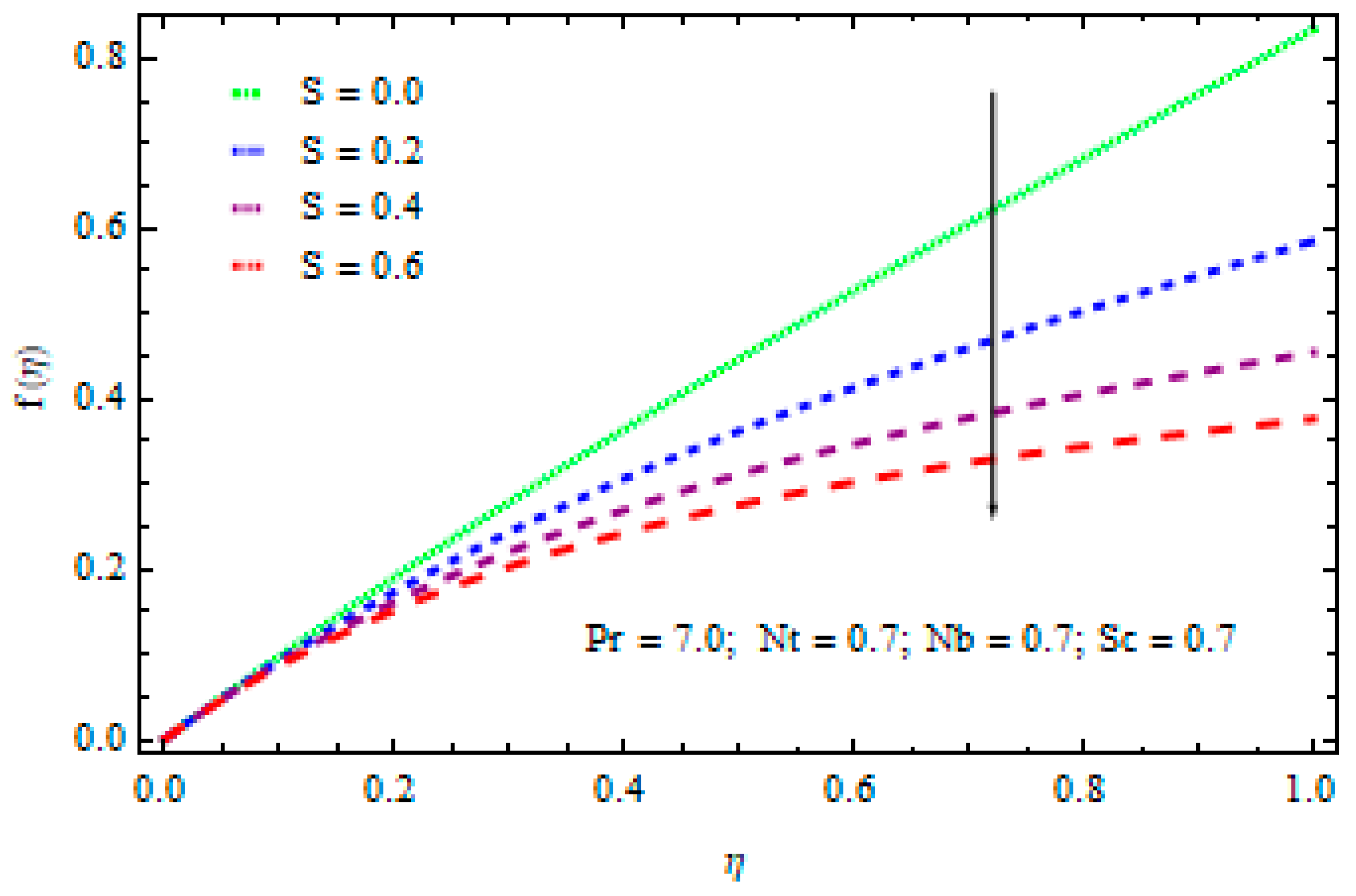
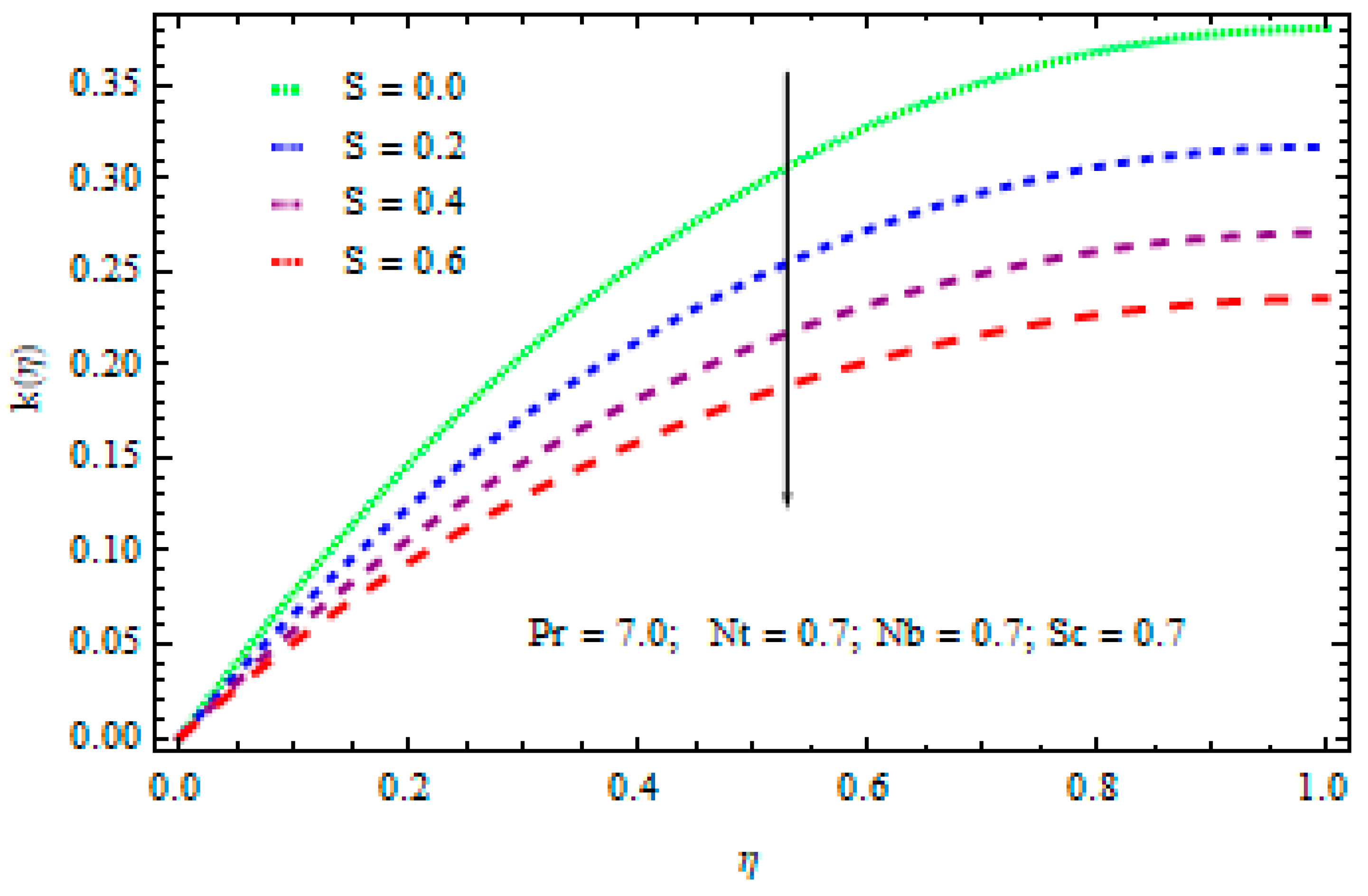
- The increase in unsteadiness factor S increases the thickness of the momentum boundary layer.
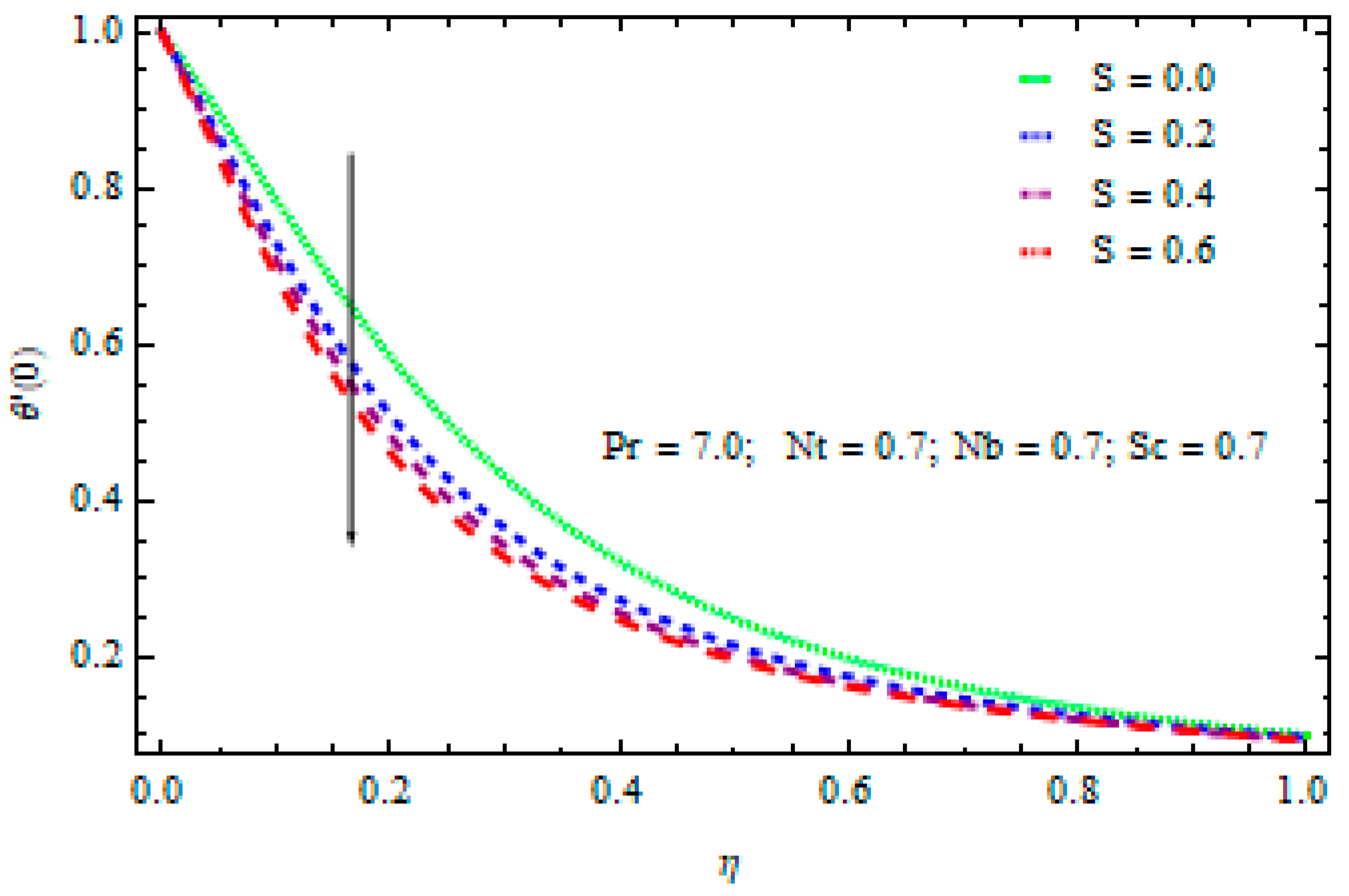
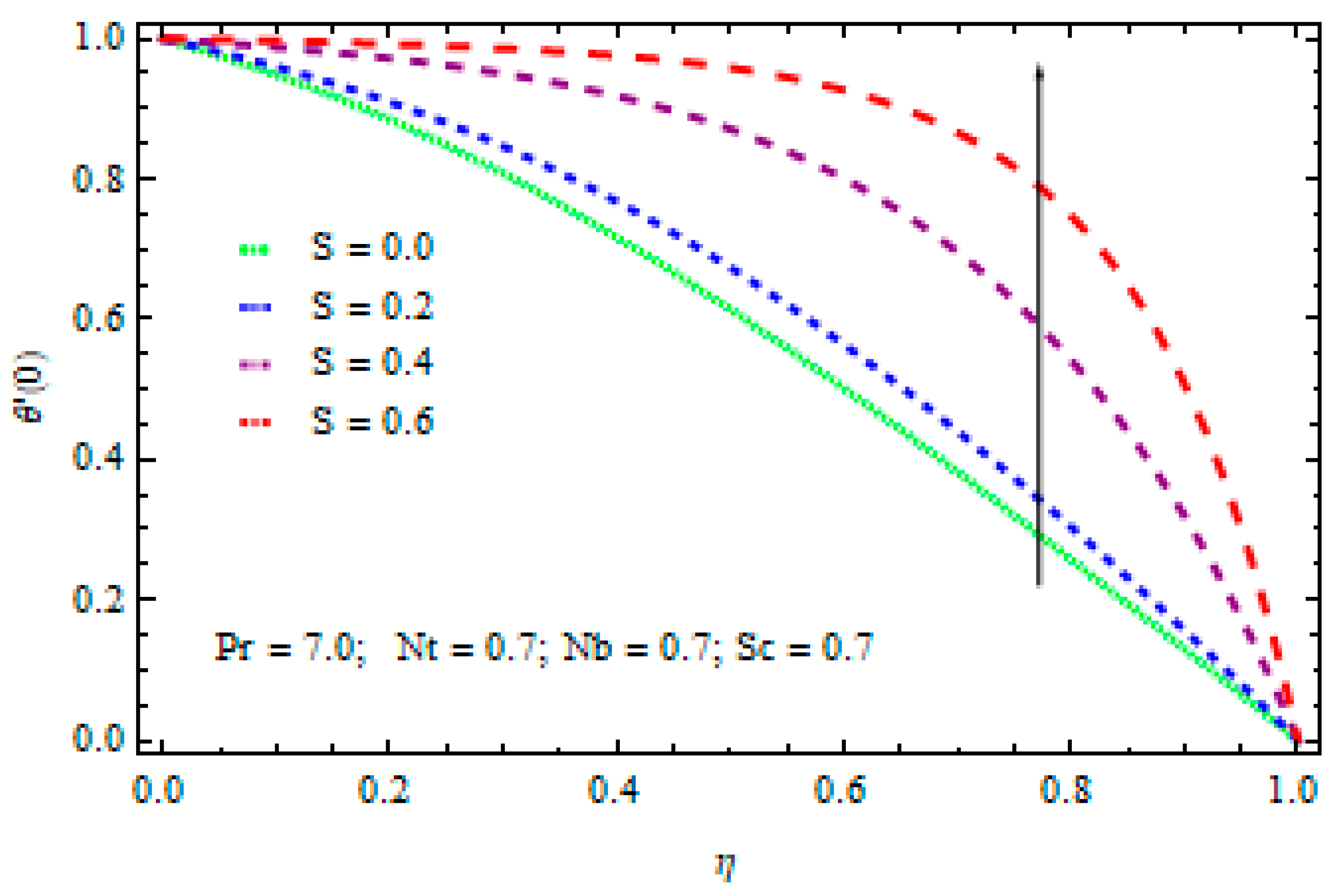
- The temperature values drop with the rise in factor S. The heat flow from sheet to fluid reduces with the rise in S and results in a cooling effect.
- The impact of the rise in the momentum boundary layer resulted from the rise in the unsteadiness parameter S.
- The rise in S decreases the temperature of the momentum boundary layer, increasing the Nusselt number. This cooling effect is delayed because of the collisions of the molecules.
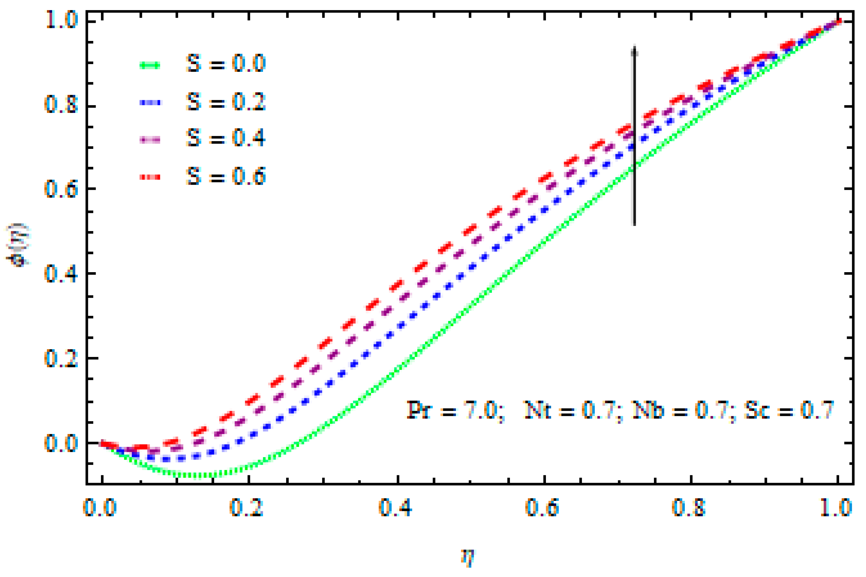
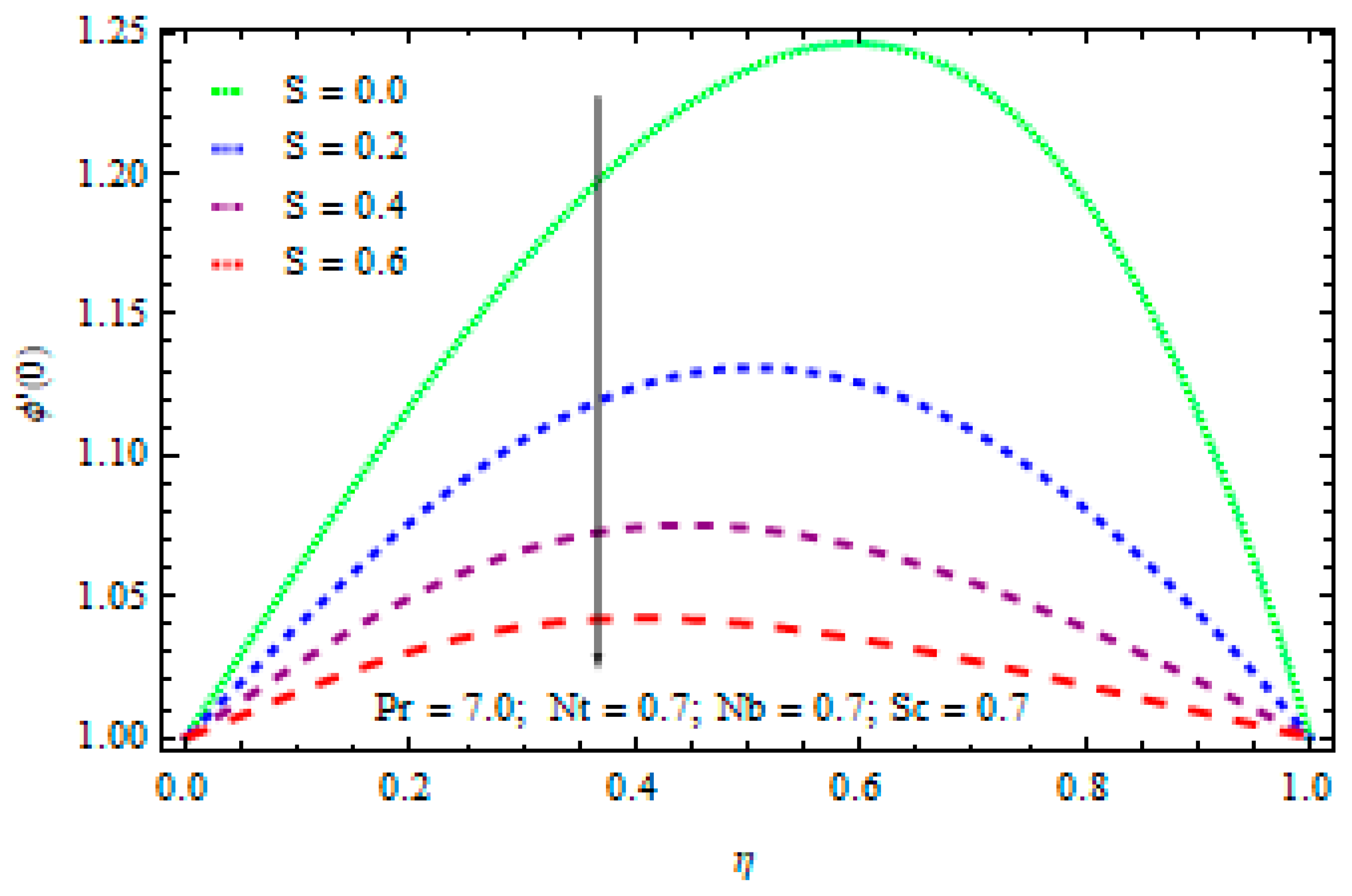
- The Sherwood number drops as the value of S increases.
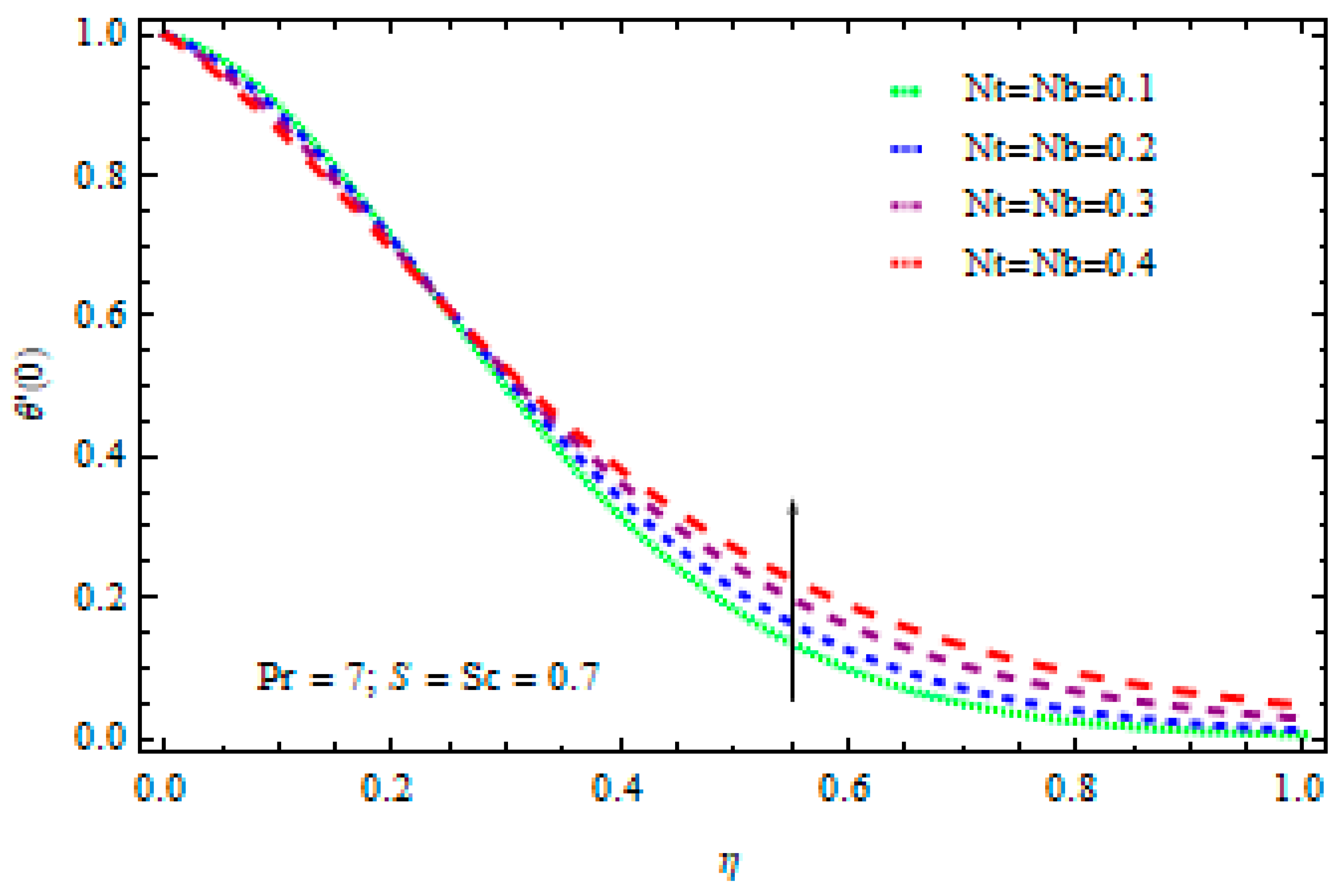
- The thickness of the thermal boundary layer increases with the increase in the Brownian motion Nb.
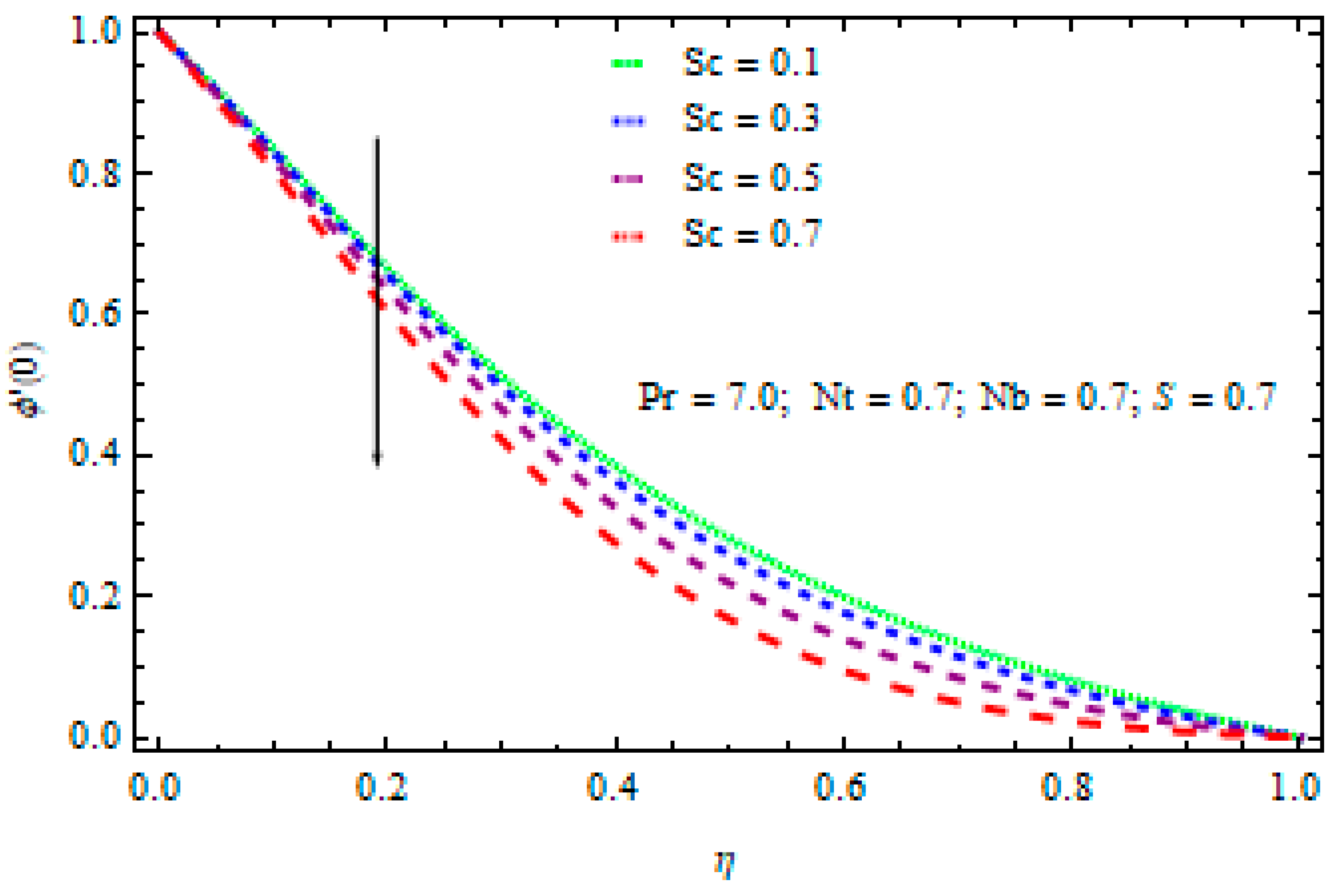
- Kinematic velocity is increased with the increase in the Schmidt number Sc. This reduces the Sherwood number because of the concentration of chemical species.
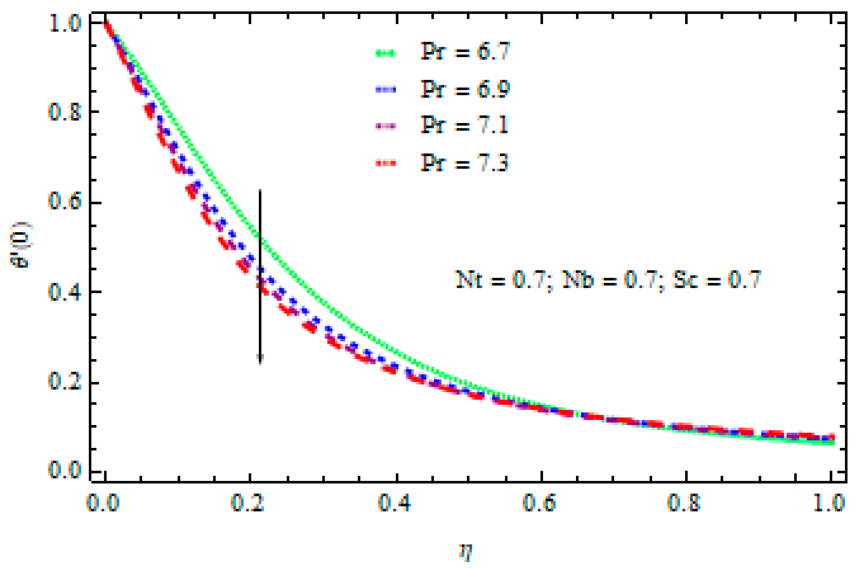
- Thickness of the thermal boundary layer increases with the increase in the Prandtl number Pr, hindering the cooling process resulting from transfer of heat.
Author Contributions
Acknowledgments
Conflicts of Interest
References
- Miladinova, S.; Lebon, G.; Toshev, E. Thin film flow of a power law liquid falling down an inclined plate. J. Non-Newton. Fluid Mech. 2004, 122, 69–78. [Google Scholar] [CrossRef]
- Gul, T.; Shah, R.A.; Islam, S.; Arif, M. MHD thin film flows of a third-grade fluid on a vertical belt with slip boundary conditions. J. Appl. Math. 2013, 2013, 707286. [Google Scholar] [CrossRef]
- Khaled, A.R.; Vafai, K. Hydrodynamic squeezed flow and heat transfer over a sensor surface. Int. J. Eng. Sci. 2004, 42, 509–519. [Google Scholar] [CrossRef]
- Siddiqui, A.M.; Ahmed, M.; Ghori, Q.K. Thin film flow of non-Newtonian fluid on a moving belt. Chaos Sol. Fract. 2007, 33, 1006–1016. [Google Scholar] [CrossRef]
- Siddiqui, A.M.; Mahmood, R.; Ghori, Q.K. Homotopy perturbation method for thin film flow of a fourth-grade fluid down a vertical cylinder. Phys. Lett. A 2006, 352, 404–410. [Google Scholar] [CrossRef]
- Costa, A.; Macedonio, G. Viscous heating in fluids with temperature dependent viscosity implications for magma flows. Nonlinear Proc. Geophys. 2003, 10, 545–555. [Google Scholar] [CrossRef]
- Nadeem, S.; Awais, M. Thin film flow of an unsteady shrinking sheet through porous medium with variable viscosity. Phys. Lett. A 2008, 372, 4965–4972. [Google Scholar] [CrossRef]
- Ellahi, R.; Riaz, A. Analytical solution for MHD flow in a third-grade fluid with variable viscosity. Math. Comput. Mod. 2010, 52, 1783–1793. [Google Scholar] [CrossRef]
- Aksoy, Y.; Pakdemirly, M. Approximate analytical solution for flow of a third-grade fluid through a parallel-plate channel filled with a porous medium. Transp. Porous 2010, 83, 375–395. [Google Scholar] [CrossRef]
- Sheikholeslami, M.; Hatami, M.; Ganji, D.D. Numerical investigation of nanofluid spraying on an inclined rotating disk for cooling process. J. Mol. Liq. 2015, 211, 577–583. [Google Scholar] [CrossRef]
- Vajravelu, K.; Sreenadh, S.; Saravana, R. Influence of velocity slip and temperature jump conditions on the peristaltic flow of a Jeffrey fluid in contact with a Newtonian fluid. Appl. Math. Nonlinear Sci. 2017, 2, 429–442. [Google Scholar] [CrossRef]
- Prasad, K.V.; Vaidya, H.; Vajravelu, K. MHD mixed convection heat transfer over a non-linear slender elastic sheet with variable fluid properties. Appl. Math. Nonlinear Sci. 2017, 2, 351–366. [Google Scholar] [CrossRef]
- Awati, V.B. Dirichlet series and analytical solutions of MHD viscous flow with suction/blowing. Appl. Math. Nonlinear Sci. 2017, 2, 341–350. [Google Scholar] [CrossRef]
- Attia, H.A. Unsteady MHD flow near a rotating porous disk with uniform suction or injection. Fluid Dyn. Res. 1998, 23, 283–290. [Google Scholar] [CrossRef]
- Freidoonimehr, N.; Rashidi, M.M.; Mahmud, S. Unsteady MHD free convective flow past a permeable stretching vertical surface in a nano-fluid. Int. J. Therm. Sci. 2015, 87, 136–145. [Google Scholar] [CrossRef]
- Makinde, O.D.; Mabood, F.; Khan, W.A.; Tshehla, M.S. MHD flow of a variable viscosity nanofluid over a radially stretching convective surface with radiative heat. J. Mol. Liq. 2016, 219, 624–630. [Google Scholar] [CrossRef]
- Akbar, T.; Batool, S.; Nawaz, R.; Zia, Q.M.Z. Magnetohydrodynamics flow of nanofluid due to stretching/shrinking surface with slip effect. Adv. Mech. Eng. 2017, 9. [Google Scholar] [CrossRef]
- Ramzan, M.; Chung, J.D.; Ullah, N. Partial slip effect in the flow of MHD micropolar nanofluid flow due to a rotating disk—A numerical approach. Results Phys. 2017, 7, 3557–3566. [Google Scholar] [CrossRef]
- Hilfer, R. Applications of Fractional Calculus in Physics; World Scientific Publishing Company: Singapore, 2000; pp. 87–130. [Google Scholar]
- Sabatelli, L.; Keating, S.; Dudley, J.; Richmond, P. Waiting time distributions in financial markets. Eur. Phys. J. B 2002, 27, 273–275. [Google Scholar] [CrossRef]
- Metler, R.; Klafter, J. The random walk’s guide to anomalous diffusion: A fractional dynamics approach. Phys. Rep. 2000, 339, 1–77. [Google Scholar] [CrossRef]
- Khan, Z.; Rasheed, H.; Tlili, I.; Khan, I.; Abbas, T. Runge-Kutta 4th-order method analysis for viscoelastic Oldroyd 8-constant fluid used as coating material for wire with temperature dependent viscosity. Sci. Rep. 2018. [Google Scholar] [CrossRef] [PubMed]
- Khan, Z.; Rasheed, H.; Ullah, M.; Gul, T.; Jan, A. Analytical and numerical solutions of Oldroyd 8-constant fluid in double-layer optical fiber coating. J. Coat. Technol. Res. 2019, 16, 235–248. [Google Scholar] [CrossRef]
- Khan, M.; Abbas, Q.; Duru, K. Magnetohydrodynamic flow of a Sisko fluid in annular pipe: A numerical study. Int. J. Numer. Meth. Fluids 2010, 62, 1169–1180. [Google Scholar] [CrossRef]
- Saeed, A.; Shah, Z.; Islam, S.; Jawad, M.; Ullah, A.; Gul, T.; Kumam, P. Three-Dimensional Casson Nanofluid Thin Film Flow over an Inclined Rotating Disk with the Impact of Heat Generation/Consumption and Thermal Radiation. Coatings 2019, 9, 248. [Google Scholar] [CrossRef]
- Binding, D.M.; Blythe, A.R.; Guster, S.; Mosquera, A.A.; Townsend, P.; Wester, M.P. Modelling polymer melt flows in wire coating process. J. Non-Newton. Fluid Mech. 1996, 64, 191–206. [Google Scholar] [CrossRef]
- Nayak, M.; Dash, G.C.; Singh, L.P. Steady MHD flow and heat transfer of a third grade fluid in a wire coating analysis with temperature dependent viscosity. Int. J. Heat Mass Transf. 2014, 79, 1087–1095. [Google Scholar] [CrossRef]
- Salem, A.M. Variable viscous and thermal conductivity effect on MHD flow and heat transfer in viscoelastic fluid over a stretching sheet. Phys. Lett. A 2007, 369, 315–322. [Google Scholar] [CrossRef]
- Bhukta, D.; Dash, G.C.; Mishra, S.R.; Baag, S. Dissipation effect on MHD mixed convection flow over a stretching sheet through porous medium with non-uniform heat source/sink. Ain Shams Eng. J. 2015, 8, 353–361. [Google Scholar] [CrossRef]
- Majeed, A.; Zeeshan, A.; Ellahi, R. Unsteady ferromagnetic liquid flow and heat transfer analysis over a stretching sheet with the effect of dipole and prescribed heat flux. J. Mol. Liq. 2016, 223, 528–533. [Google Scholar] [CrossRef]
- Liao, S.J. Beyond Perturbation: Introduction to Homotopy Analysis Method; Chapman and Hall, CRC Press: Boca Raton, FL, USA, 2003. [Google Scholar]
- Liao, S.J. Homotopy Analysis Method in Non-Linear Differential Equations; Springer and Higher Education Press: Heidelberg, Germany, 2012. [Google Scholar]
- Khan, Z.; Khan, M.A.; Siddiqui, N.; Ullah, M.; Shah, Q. Solution of magnetohydrodynamic flow and heat transfer of radiative viscoelastic fluid with temperature dependent viscosity in wire coating analysis. PLoS ONE 2018, 13, e0194196. [Google Scholar] [CrossRef] [PubMed]
- Khan, Z.; Rasheed, H.; Alkanhal, T.A.; Ullah, M.; Khan, I.; Tlili, I. Effect of magnetic field and heat source on Upper-convected-maxwell fluid in a porous channel. Open Phys. 2018, 16, 917–928. [Google Scholar] [CrossRef]


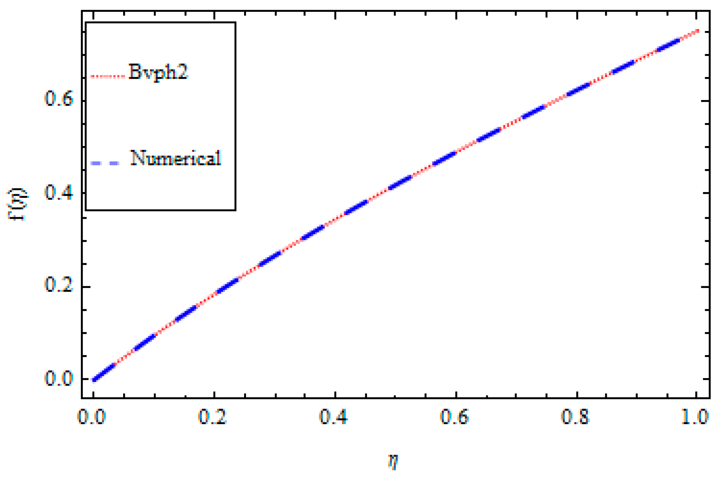
| f(η) | HAM Solution | Numerical Solution | Absolute Error |
|---|---|---|---|
| 0.0 | 0.000000 | −4.113240 × 10⁻⁹ | 4.113240 × 10⁻⁹ |
| 0.1 | 0.095967 | 0.095967 | 2.757140 × 10⁻⁹ |
| 0.2 | 0.184817 | 0.184817 | 2.395770 × 10⁻⁹ |
| 0.3 | 0.267754 | 0.267754 | 1.427160 × 10⁻⁹ |
| 0.4 | 0.345761 | 0.345761 | 9.250300 × 10⁻¹⁰ |
| 0.5 | 0.419668 | 0.419668 | 6.552510 × 10⁻¹⁰ |
| 0.6 | 0.490197 | 0.490197 | 2.840370 × 10⁻¹⁰ |
| 0.7 | 0.558005 | 0.558005 | 9.286170 × 10⁻¹⁰ |
| 0.8 | 0.623724 | 0.623724 | 1.115280 × 10⁻⁹ |
| 0.9 | 0.687991 | 0.687991 | 6.833170 × 10⁻¹⁰ |
| 1.0 | 0.751489 | 0.751489 | 2.694550 × 10⁻¹⁰ |
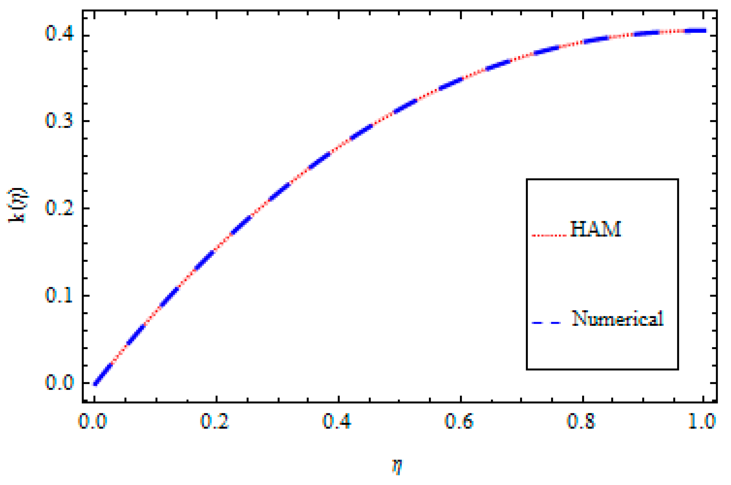
| k(η) | HAM Solution | Numerical Solution | Absolute Error |
|---|---|---|---|
| 0.0 | 0.000000 | 8.431700 × 10⁻¹¹ | 8.431700 × 10⁻¹¹ |
| 0.1 | 0.083047 | 0.083047 | 8.194100 × 10⁻¹⁰ |
| 0.2 | 0.156141 | 0.156141 | 1.507400 × 10⁻⁹ |
| 0.3 | 0.218995 | 0.218995 | 2.567920 × 10⁻⁹ |
| 0.4 | 0.271888 | 0.271888 | 3.456570 × 10⁻⁹ |
| 0.5 | 0.315142 | 0.315142 | 4.203450 × 10⁻⁹ |
| 0.6 | 0.349196 | 0.349196 | 4.967530 × 10⁻⁹ |
| 0.7 | 0.374581 | 0.374581 | 5.555180 × 10⁻⁹ |
| 0.8 | 0.391897 | 0.391897 | 5.900650 × 10⁻⁹ |
| 0.9 | 0.401789 | 0.401789 | 6.210250 × 10⁻⁹ |
| 1.0 | 0.404932 | 0.404932 | 1.059580 × 10⁻⁸ |
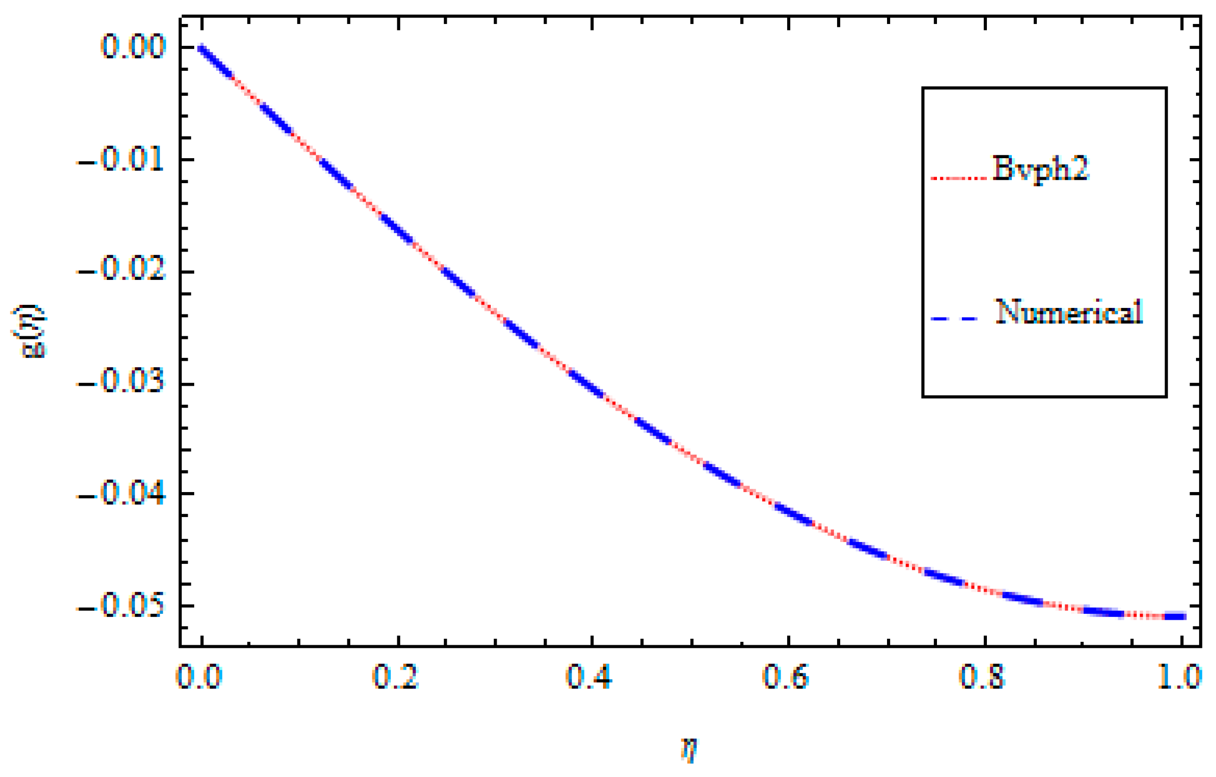
| g(η) | HAM Solution | Numerical Solution | Absolute Error |
|---|---|---|---|
| 0.0 | 0.000000 | −8.866030 × 10⁻¹¹ | 8.866030 × 10⁻¹⁰ |
| 0.1 | -0.008248 | −0.008248 | 1.092590 × 10⁻¹⁰ |
| 0.2 | -0.016231 | −0.016231 | 6.850590 × 10⁻¹⁰ |
| 0.3 | -0.023721 | −0.023721 | 1.199930 × 10⁻¹⁰ |
| 0.4 | -0.030534 | −0.030534 | 1.572520 × 10⁻¹⁰ |
| 0.5 | -0.036521 | −0.036521 | 1.944400 × 10⁻¹⁰ |
| 0.6 | -0.041566 | −0.041566 | 2.672430 × 10⁻¹⁰ |
| 0.7 | -0.045583 | −0.045583 | 3.628050 × 10⁻¹⁰ |
| 0.8 | -0.048506 | −0.048506 | 3.482500 × 10⁻¹⁰ |
| 0.9 | -0.050288 | −0.050288 | 3.068110 × 10⁻¹⁰ |
| 1.0 | -0.050890 | −0.050890 | 7.346430 × 10⁻¹⁰ |
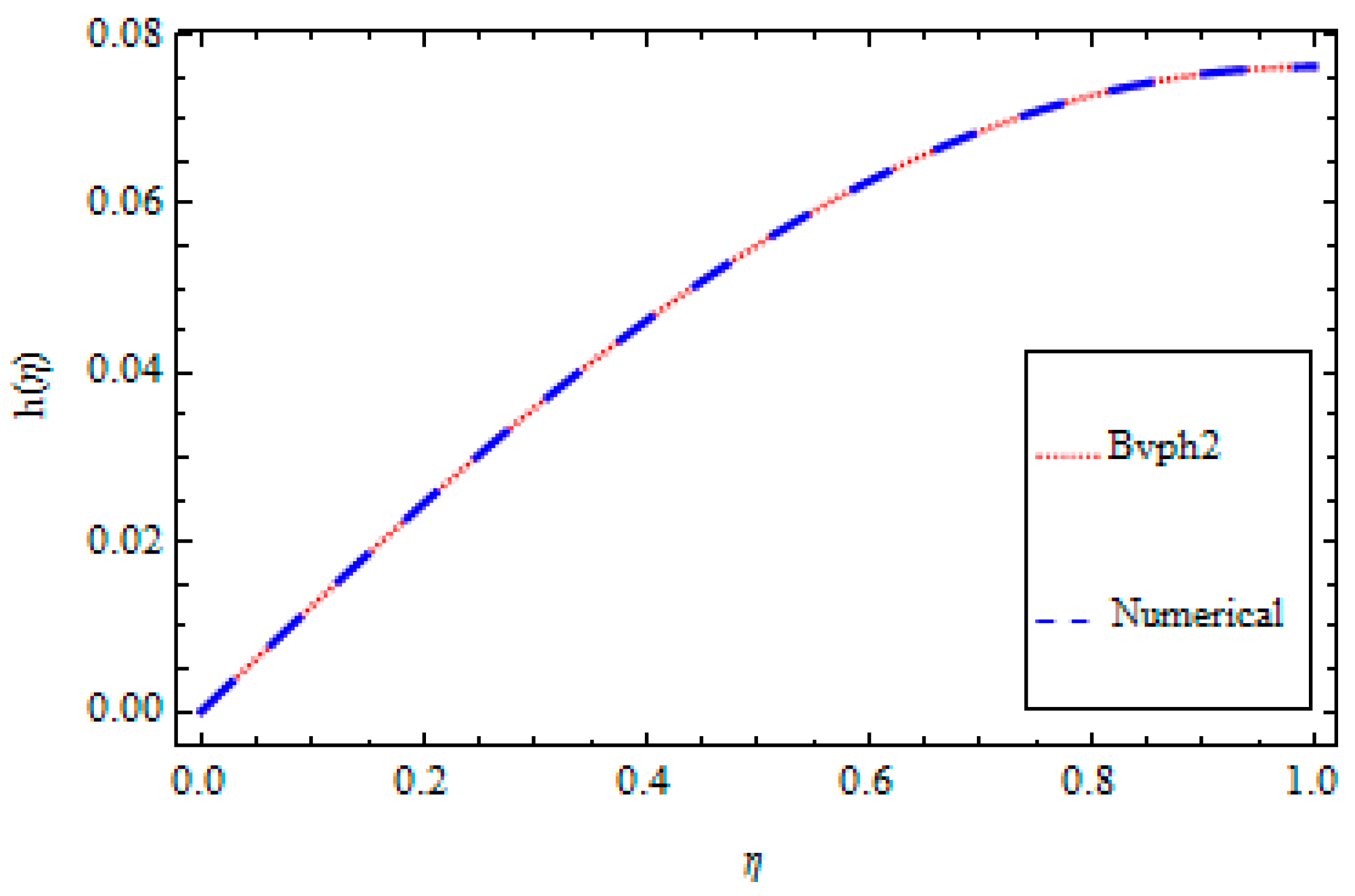
| h(η) | HAM Solution | Numerical Solution | Absolute Error |
|---|---|---|---|
| 0.0 | 0.000000 | −6.298860 × 10⁻¹¹ | 6.298860 × 10⁻¹¹ |
| 0.1 | 0.012496 | 0.012496 | 4.280720 × 10⁻¹¹ |
| 0.2 | 0.024589 | 0.024589 | 4.879770 × 10⁻¹¹ |
| 0.3 | 0.035923 | 0.035923 | 1.257860 × 10⁻¹¹ |
| 0.4 | 0.046200 | 0.046200 | 9.318280 × 10⁻¹¹ |
| 0.5 | 0.055181 | 0.055181 | 2.305180 × 10⁻¹⁰ |
| 0.6 | 0.062687 | 0.062687 | 3.234660 × 10⁻¹⁰ |
| 0.7 | 0.068598 | 0.068598 | 4.674580 × 10⁻¹⁰ |
| 0.8 | 0.072833 | 0.072833 | 6.805310 × 10⁻¹⁰ |
| 0.9 | 0.075371 | 0.075371 | 8.340060 × 10⁻¹⁰ |
| 1.0 | 0.076213 | 0.076213 | 2.122270 × 10⁻⁹ |
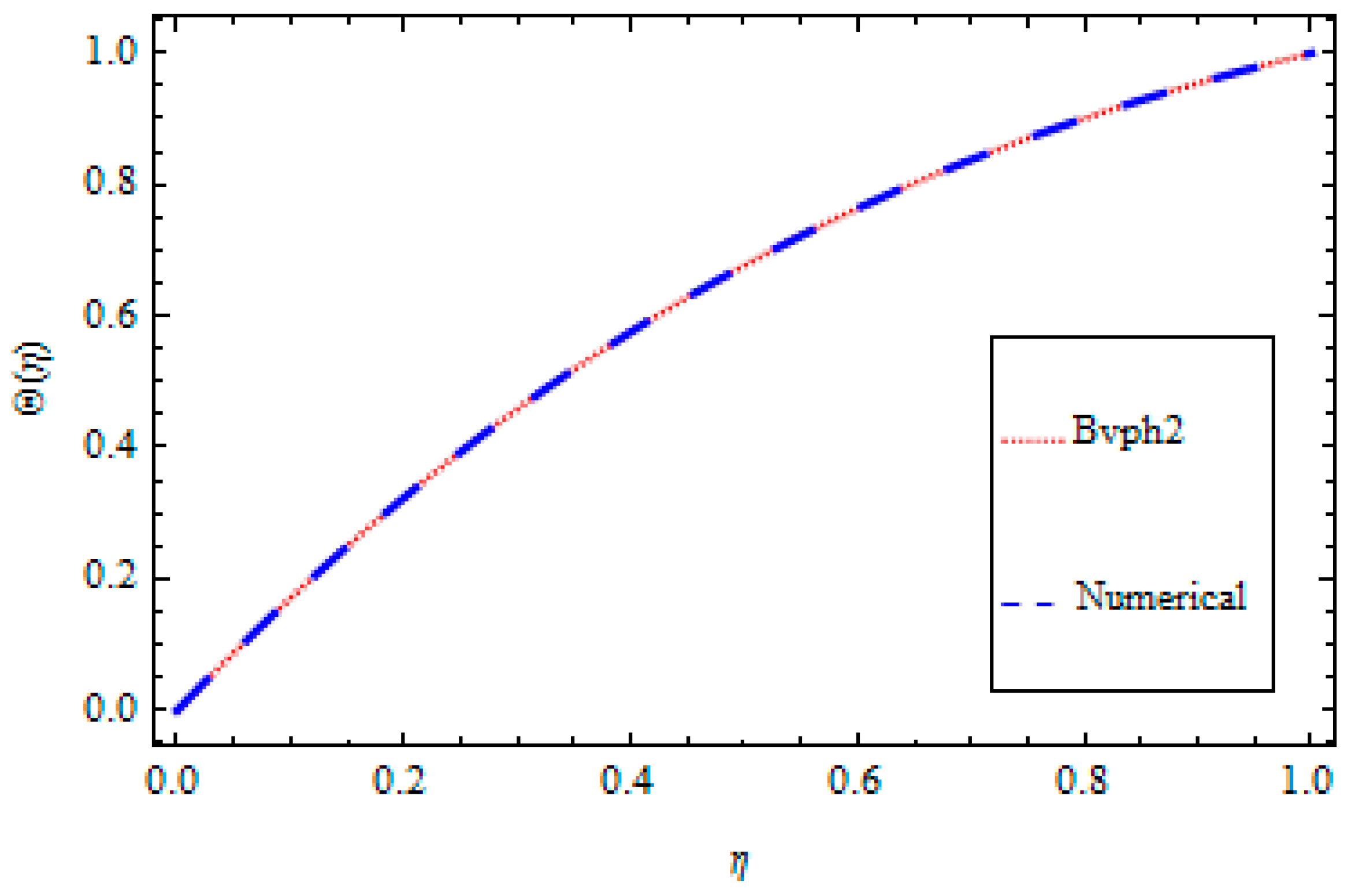
| θ(η) | HAM Solution | Numerical Solution | Absolute Error |
|---|---|---|---|
| 0.0 | 0.000000 | −8.964480 × 10⁻⁹ | 8.964480 × 10⁻⁹ |
| 0.1 | 0.171025 | 0.171025 | 7.561540 × 10⁻⁹ |
| 0.2 | 0.323916 | 0.323916 | 5.991460 × 10⁻⁹ |
| 0.3 | 0.458661 | 0.458661 | 1.565540 × 10⁻⁹ |
| 0.4 | 0.576014 | 0.576014 | 5.012150 × 10⁻⁹ |
| 0.5 | 0.677270 | 0.677270 | 4.974440 × 10⁻⁹ |
| 0.6 | 0.764037 | 0.764037 | 4.021380 × 10⁻⁹ |
| 0.7 | 0.838044 | 0.838044 | 2.454450 × 10⁻¹⁰ |
| 0.8 | 0.901001 | 0.901001 | 2.836300 × 10⁻⁹ |
| 0.9 | 0.954508 | 0.954508 | 4.201010 × 10⁻⁹ |
| 1.0 | 1.000000 | 1.000000 | 1.110220 × 10⁻¹⁶ |
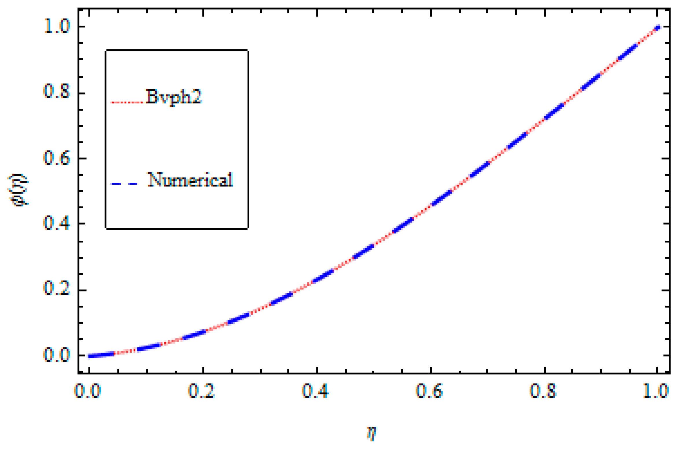
| ϕ(η) | HAM Solution | Numerical Solution | Absolute Error |
|---|---|---|---|
| 0.0 | 0.000000 | 2.528420 × 10⁻⁸ | 2.528420 × 10⁻⁸ |
| 0.1 | 0.025998 | 0.025998 | 2.009500 × 10⁻⁸ |
| 0.2 | 0.074274 | 0.074274 | 1.458960 × 10⁻⁸ |
| 0.3 | 0.144049 | 0.144049 | 5.628440 × 10⁻⁸ |
| 0.4 | 0.233238 | 0.233238 | 1.590860 × 10⁻⁸ |
| 0.5 | 0.338896 | 0.338896 | 1.758020 × 10⁻⁸ |
| 0.6 | 0.457662 | 0.457662 | 1.656760 × 10⁻⁸ |
| 0.7 | 0.586132 | 0.586132 | 8.921160 × 10⁻⁹ |
| 0.8 | 0.721129 | 0.721129 | 3.159840 × 10⁻⁹ |
| 0.9 | 0.589864 | 0.589864 | 1.324590 × 10⁻⁹ |
| 1.0 | 1.000000 | 1.000000 | 2.220450 × 10⁻¹⁶ |
© 2019 by the authors. Licensee MDPI, Basel, Switzerland. This article is an open access article distributed under the terms and conditions of the Creative Commons Attribution (CC BY) license (http://creativecommons.org/licenses/by/4.0/).
Share and Cite
Rasheed, H.U.; Khan, Z.; Khan, I.; Ching, D.L.C.; Nisar, K.S. Numerical and Analytical Investigation of an Unsteady Thin Film Nanofluid Flow over an Angular Surface. Processes 2019, 7, 486. https://doi.org/10.3390/pr7080486
Rasheed HU, Khan Z, Khan I, Ching DLC, Nisar KS. Numerical and Analytical Investigation of an Unsteady Thin Film Nanofluid Flow over an Angular Surface. Processes. 2019; 7(8):486. https://doi.org/10.3390/pr7080486
Chicago/Turabian StyleRasheed, Haroon Ur, Zeeshan Khan, Ilyas Khan, Dennis Ling Chuan Ching, and Kottakkaran Sooppy Nisar. 2019. "Numerical and Analytical Investigation of an Unsteady Thin Film Nanofluid Flow over an Angular Surface" Processes 7, no. 8: 486. https://doi.org/10.3390/pr7080486
APA StyleRasheed, H. U., Khan, Z., Khan, I., Ching, D. L. C., & Nisar, K. S. (2019). Numerical and Analytical Investigation of an Unsteady Thin Film Nanofluid Flow over an Angular Surface. Processes, 7(8), 486. https://doi.org/10.3390/pr7080486