Ear Detection and Localization with Convolutional Neural Networks in Natural Images and Videos

Abstract

The difficulty in precisely detecting and locating an ear within an image is the first step to tackle in an ear-based biometric recognition system, a challenge which increases in difficulty when working with variable photographic conditions. This is in part due to the irregular shapes of human ears, but also because of variable lighting conditions and the ever changing profile shape of an ear’s projection when photographed. An ear detection system involving multiple convolutional neural networks and a detection grouping algorithm is proposed to identify the presence and location of an ear in a given input image. The proposed method matches the performance of other methods when analyzed against clean and purpose-shot photographs, reaching an accuracy of upwards of 98%, but clearly outperforms them with a rate of over 86% when the system is subjected to non-cooperative natural images where the subject appears in challenging orientations and photographic conditions.

1. Introduction

The problem of people recognition by means of identifying them biometrically by their ear has received considerable attention in the literature. Forensic science has often used a person’s ear to establish someone’s identity, and considerable improvements are being made in this field to improve these systems—more so now that it starts to be implemented as a new method for biometric recognition [1]. However, for an ear recognition system to be accurate, the first and obvious step it must take is to properly detect the presence and location of an ear within an image frame. This seemingly simple task is often made more difficult because in practice, such images very commonly present the subject’s ear in poses which are much different to those a system is usually trained for. Furthermore, occlusion and partially visible ears is very common in natural images, and it presents a challenge which must be addressed.

The Convolutional Neural Network (CNN) [2] is considered today to be one of the broadest and most adaptable visual recognition systems, especially in the case where the imagery is highly variable in form, illumination, and even perspective. A standard CNN is made up two sequential parts, the first one is in charge of feature extraction and learning based on these features, while the second one is (usually) dedicated to classification and the final recognition of the object of interest. A gradient descent algorithm [3] can be used to train these two stages together, end-to-end, and it is precisely this characteristic which gives CNNs their power and flexiblity. This type of networks have, in recent years, come to almost entirely replace other machine learning systems. This is especially the case in image recognition tasks over large datasets [4]. These systems are even capable of performing better than humans can when manually classifying large image datasets [5]. In this work, we exploit the flexible architecture of CNNs to apply them in a custom-designed manner to the particular task of human ear recognition.

The article follows this outline: Section 2 presents a review on the existing methods for the detection of ears and describes the current state of the art. A brief review and explanation of typical CNN architectures is also given. Section 3 describes the methodology our proposed system follows; Section 4 discusses the results and compares them qualitatively to existing methods; and finally Section 5 gives our conclusions and discusses future lines of work that will follow from this research.

2. Background

2.1. Ear Detection State of the Art

Most systems that do ear detection rely on properties in the geometry and morphology of the ear, such as in specific features being visible, or patterns in frequency of low level features. Considerable progress has been made recently in the area of biometrics related to the human ear. One of the best known techniques for ear detection was given by Burge and Burger [6] who proposed a system that makes use of deforming contours, although it does need user input for initializing a contour. As a result, the localization process with this system is not truly automated. Hurley et al. [7] uses force fields, and in this process the location of the ear is not necessary as input in order to do the recognition; however, this technique is very sensitive to noise and requires a clean image of the ear to perform well. In [8], Yan and Bowyer uses a technique that requires two user defined lines to carry out the detection, which again is not fully automated—as one of the input lines must run along the boudnary between the ear and the face, and the second line must cross vertically through the ear, thereby providing a rough localization of the ear as input to the system.

Three additional techniques are given by Chen and Bhanu for the task of ear detection. First of all, they develop a classifying system that can recognize a varying shape indices [9]. This technique, however, only works on images of a side view of the face and is furthermore not very robust against variations in perspective or scale. They also proposed a system that analyzes individual image patches that exhibit a large amount of local curvature. This system makes use of “Step Edge Magnitude”, as the technique is called [10]. This system is template-based, requiring a stencil for the usual outline shape of the helix and anti-helix of the ear, this template is then fitted to line clusters. One final technique they propsed reduces the possible number of ear detection candidates by detecting patches of skin texture as an initial step before applying a similar helix stencil matching system to the local curvatures [11].

Another example for detection is described by Attrachi et al. [12] who use contour lines to detect the ear. They locate the outer contour by performing a search on the image for the longest single connected edge feature in the image. By selecting three keypoints for the top, bottom, and left of the localized region. Image alignment can then be done by forming a triangle, such that its barycenter can be used as alignment reference. A. Cummings et al. [13] propse a techinque based on image ray transform that finds the specific tubular shape of an ear. This system relies on the helical/elliptical shape of the ear for localizing it. Kumar et al. [14] created a technique that starts by segmenting the skin, then creates an edge map with which it can finally localize the ear within the input image. They then proceed to use active contours [15] to get a more precise location of each contour.

While there are many proposals attempting to solve the problem of ear detection, only a small portion of them has been described here. An overview is presented in

Table 1. Existing ear detection approaches.

Publication	Detection Approach	Database Size	Accuracy Rate (%)
Abaza et al. [17]	Cascaded Adaboost	940	$88.72$
Ansari and Gupta [18]	Edge Detection and Curvature Estimation	700	$93.34$
Alvarez et al. [19]	Ovoid Model	$N/A$	$N/A$
Arbab-Zavar & Nixon [20]	Hough Transform	942	91
Arbab-Zavar & Nixon [21]	Log-Gabor Filters and Wavelet Transform	252	$88.4$
Attarchi et al. [12]	Edge Detection and Line Tracing	308	$98.05$
Chen & Bhanu [9]	Template Matching with Shape Index Histograms	60	$91.5$
Cummings et al. [13]	Ray Transform	252	$98.4$
Islam et al. [22]	Adaboost	942	$99.89$
Jeges & Mate [23]	Edge Orientation Pattern	330	100
Kumar et al. [14]	Edge Clustering and Active Contours	700	$94.29$
Liu & Liu [24]	Adaboost and Skin Color Filtering	50	96
Prakash & Gupta [25]	Skin Color and Graph Matching	1780	$96.63$
Shih et al. [26]	Arc-Masking and AdaBoost	376	100
Yan & Bowyer [27]	Concha Detection and ActiveContours	415	$97.6$
Yuan & Mu [28]	CAMSHIFT and a Contour Fitting	$Video$	$N/A$

outlining the best known methods, along with their reported accuracy rates, when available. A deeper review is also given in [16].

An issue to consider is the great importance of robustness against pose variation and occlusion when an ear detection algorithm is put to practice. It is worthwhile to note that most of the detection systems listed above are not tested nor developed for difficult occlusion scenarios, such as partial occlusion by the hair, jewelry, or even hats and other accessories. The most likely reason is simply the lack of public datasets containing appropriately occluded images. Furthermore, to the best of our knowledge, there is no major research that has been performed on the effect of ear occlusion in natural images.

Additionally, there does not seem to exist any approaches for the specific task of ear detection based on CNNs. Not surprisingly, as CNNs have only started to become popular relatively recently, and the extent of biometric applications using this type of system has so far been limited to full face detection, for example [29].

2.2. Convolutional Neural Networks and Shared Maps

This work is based mainly on a neural network that does classification as its main task. This is a standard CNN with an architecture composed of convolutional and max-pooling layers in alternating order as part of the feature extractor stage. After this, a few fully connected linear layers make up the the final classification network stage.

The network’s first/input layer always consists of at one or more units that contain the input image data to be analyzed. For this task, the input consists of a single grayscale channel as input data to the system.

Data next travels to each of the feature extraction stages. The first part of every such stage is a convolutional layer, wherein each neuron linearly combines the convolution of one or more maps from the preceding layer, and then passes the output through a nonlinearity function such as $tanh\left(x\right)$. A convolutional layer is usually paired with a max-pooling layer which primarily reduces the dimensionality of the data. A neuron in this type of layer acts on a single map from the corresponding incoming convolutional neuron of the previous layer, and its task is to pool several adjacent values in the map for every sampling pixel in the neuron. The sampling function used takes the maximum value among the pooled region.

The information then travels to one or more additional feature extraction stages, each of which works in a very similar manner as that described above. The result of this is that every stage extracts more and more abstract features that can eventually be used to classify the input, a process done in the final stage of the network. This consists of linear layers which ultimately classify the extracted features on the previous layered stages through a linear combination similar to a traditional multi-layer perceptron.

At the end, the output of the final layer doing the classification finally selects the class that best matches the input data image, based on the predetermined annotation labels with which the system was trained. The output of the network is composed of multiple numeric values, each one giving a probability-like expectancy of the image belonging to the particular class associated with each corresponding estimate.

Recognition of images with dimensions bigger than the input data size with which a CNN was trained with can be achieved by using sliding windows. This is defined by two parameters: S is the size of the window to use, which is set to the network’s original input data size; T is the window stride, a value that specifies how far apart sequential windows are spaced. As a result, the stride parameter defines the number of individual windows that must be analyzed for a given input. It is therefore necessary to choose an optimal value for the stride, since this amount is inversely proportional to the classifier “resolution”, in other words the resolving power of fine featues in the image. The resolution, in turn, also determines the computing resources necessary to analyze the number of windows W, as more windows obviously require more computations. For an image of size $I_w\times I_h$, the number of windows is determined as follows:

$$W=\left(\frac{I_w-S}{T}+1\right)\left(\frac{I_h-S}{T}+1\right)\Rightarrow W\propto \frac{I_w{I}_h}{T^2}$$

(1)

As an example: Taking an input image that has been downsampled to $640\times 360$, individual windows can be defined, each one of size $S=64$. To simplify calculations, a stride value of $T=S/2=32$ can be used. In this case, a network would require 190 executions to fully analyze each extracted window at this scale. If a smaller stride is used, the computation requirement increases. For example reducing the stride to $T=S/8=8$, results in over 2700 individual CNN executions. Taking into account that a single CNN execution, due to its complex nature, can require several million floating point operations, it can be seen that a dense window stride value can increase exponentially the computing toll on the system.

This process can be greatly optimized by executing the network as Shared Maps, a detailed explanation of which is given in [30]. This allows executing the network for the entire image frame in parallel, thus requiring a single execution. Although, a shared map execution of the CNN is higher in computational cost than that of a single window, it can still save on the total computing resources required for the full image by not requiring to re-analyze overlapping regions of adjacent windows, resulting in speed-ups of up to 30x. This process is exploited at its fullest potential here, and its implications are taken into account when designing the structure of the network for this task, as will be described later in this work.

3. System Description

3.1. Datasets

The existence of ear-centric data is limited and sparse. There exist no standard datasets upon which a large body of work can be contrasted with. As a result, there is great difficulty in properly comparing the system we propose with those described in Section 2, as they primarily use private data.

In this work, however, we attempt to use a variety of datasets in order to establish some benchmarks upon which future works can be built upon. For this purpose, we use a total of four datasets in our experiments. Three of these are public and only one is private. Each of these datasets has a set of features which make them particularly useful for a particular task, and each one introduces new challenges. As such, we use them all to base a selection of real-world experiments on each.

Table 2. Details on the contents of the various datasets used in this work.

Dataset	Dataset Size	Subjects	Images per Subject	Resolution Size Pixels	Color Channels	Content	Source
AMI [31]	700	100	7	$492\times 702$	$Color$	Closeup ears, both sides	$Photo$
UND [32,33]	464	114	4	$1200\times 1600$	$Color$	Bust profile, right side only	$Photo$
Videos (Train)	950	5	190	$1920\times 1080$	$Color$	Head profile, both sides	$Video$
Videos (Test)	910	7	130	$1920\times 1080$	$Color$	Head profile, both sides	$Video$
UBEAR v1.0 [34] (Train)	4497	127	35	$1280\times 960$	$Grayscale$	Head profile, both sides, and masks	$Video$
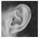
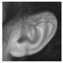
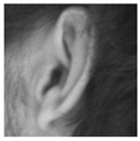
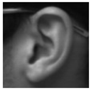
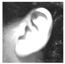
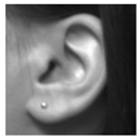
UBEAR v1.1 [34] (Test)	4624	115	40	$1280\times 960$	$Grayscale$	Head profile, both sides	$Video$

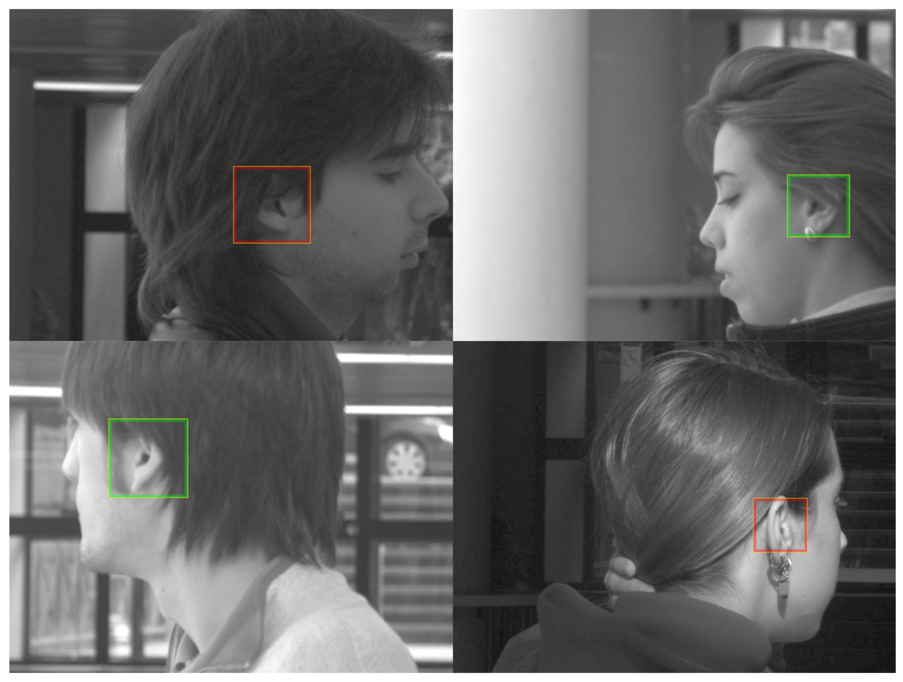
gives an overview of the content in each dataset, and Figure 1 displays some samples of each to qualitatively demonstrate their contents.

The first dataset is the AMI dataset [31], a collection of 700 closeup images of ears. These are all high quality images of ears perfectly aligned and centered in the image frame, as well as having high photographic quality, in good illumination conditions and all in good focus. This dataset is therefore exemplary in order to test the recognition sensitivity towards different ears, however, due to the closeup nature of the images, they are not really well suited for ear localization tasks.

The second dataset we use is the UND dataset [32,33]. A collection of photographs of multiple subjects in profile, where the ear covers only a small portion of the image. The photographic quality of these images is very high, and again all in constant and good illumination, and with none of the ears being occluded by hair or other objects. The poses of subjects varies very slightly in relation to the camera, but not so much as to introduce distracting effects due to head rotation and pose. As a result, these images are suitable in testing the specific task of localization among a large image frame, while avoiding the challenges of viewpoint and illumination variation.

The third dataset is the Video dataset. A private collection of 940 images composed of HD frames extracted from short video sequences of voluntary participants. There are 14 image sequences of 7 subjects—one for each person’s ear. Each sequence consists of 65 frames from a span of approximately 15 seconds in time extracted from a continuous video. The subjects were asked to rotate their heads in various natural poses following smooth and continuous motions throughout the sequence. The illumination and environment are relatively consistent across all videos, and subjects were asked to move any potential occlusion away from their ears. We use this dataset primarily to test the detector sensitivity only towards different relative rotations of the subject’s head in relation to the camera, while avoiding challenges due to variable illumination. The higher number of images per subject, combined with a low number of total subjects, are useful to also reduce the effect from using a large number of wildly variable ear shapes in the tests, and again, concentrate mainly on their pose. A variation of this dataset was created and set aside for training purposes. This comprised profile image frames from an additional 5 participants, different from the subjects in the test dataset.

The final and perhaps most important dataset we use is the UBEAR [34] dataset. This is a very large collection of images of subjects shot under a wide array of variations, which spans multiple dimensions—not only in pose and rotation, but also in illumination, occlusion, and even camera focus. These images, therefore, simulate to a very good degree the conditions of photographs in non-cooperative environments were natural images of people would be captured ad hoc and used to carry out such a detection. These images, although definitely being ear-centric, make no attempt at framing or capturing the ear under perfect conditions, and as such reflect a real-world test scenario. As our main interest in this work is the detection of ears in natural images, this then becomes our main dataset to test the fullest potential of the system we propose.

Table 3. Differences and challenges presented in the UBEAR dataset.

Angles
Exposure
Blur
Gender
Occlusion

gives a more in depth review on the different challenges found in this specific dataset.

It is also important to note that the UBEAR dataset comes in two versions, both of which consist of unique non-repeating images across both sets. The first of these versions, named 1.0, includes a ground truth mask outlining the exact location of the ear in each image. As will be described later, this inclusion was important for our training procedure. The other version, 1.1, does not include such masks, and is therefore reserved for testing and experimentation.

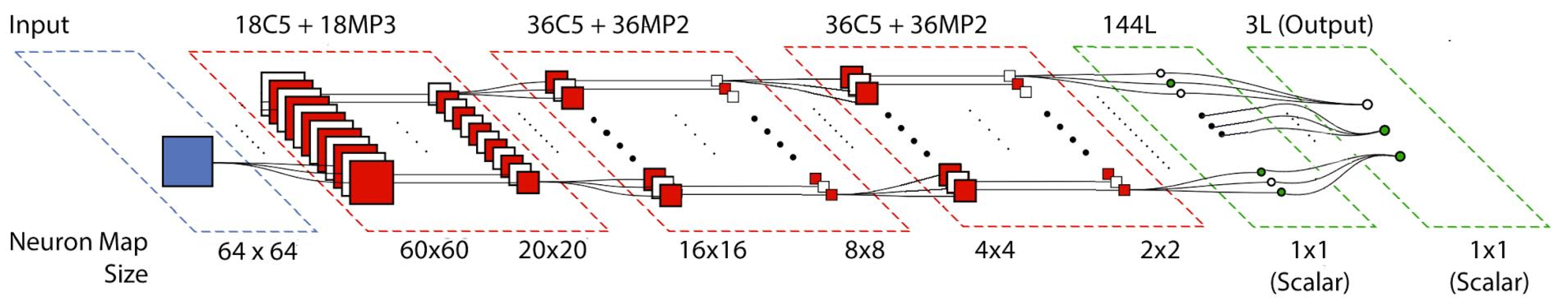
3.2. Convolutional Neural Network

The CNN used is based on a standard architecture with a few customizations made to the architecture which greatly help for the use case presented. The network architecture used is visually depicted in Figure 2.

The target use case of the system is to perform real time ear detection, especially with input video streams. For this, a system that can run quickly is a fundamental requirement. For this reason, an optimized architecture is needed. The target classes we seek to recognize with the neural network are only three: (i) Left Ear, (ii) Right Ear, and (iii) Background—referred to by their corresponding abbreviations: LE, RE, and BG in all the following descriptions of the system. As the data variability within each class is relatively low, with many training data samples having a similar set of characteristic ear features, the network can perform relatively well by learning only a small number of unique features (unlike the case of large modern CNNs). Therefore, a small neural network, with a low layer and neuron count is enough to learn the training data used by this system.

Furthermore, a size of 64×64 is selected for the input data of the network, as images at this size carry enough features and information to properly define the ear shape, while at the same time not being so large that the system would require large convolutional kernels to properly analyze the images.

Finally, as Shared Maps execution will be used to do the analysis over full images, the maximum accumulated pooling factor needs to be kept small. This ensures that the stride size on the final output map is still small for fine localization to take place. For this reason, 3 convolutional and pooling layers are decided as the base of the architecture.

Knowing these three constraints, for the input and output, and the maximum number of layers, through a process of iterative trial and error, a final architecture was decided upon as follows:

18C5:MP3 + 36C5:MP2 + 36C5:MP2 + 144L + 3L

where the notation $A(C,MP,L)B$ means a convolutional (C), max-pooling (MP) or linear (L) layer, of A neurons, and kernel size B. This architecture, when executed as Shared Maps, yields a minimum window stride size of $3\times 2\times 2=12$, which is quite efficient for purposes of detection over a half-HD image frame, as it allows analyzing the image at intervals as close as 12 pixels apart, or multiples thereof.

3.3. 3-CNN Inference

Training a single neural network and expecting it to be sufficient to properly tell apart ears from background noise in real-world imagery is quite the leap of faith.

In practice, a neural network of this type will be quite capable at properly recognizing the large majority of ear-shaped objects that are presented to it. Thus, when tested against a set of cut-out ear images specifically prepared for such a task of recognition, its true positive inference performance will be quite good. However, it will be prone to make many mistakes when presented with background images or noise. The network is trained with a BG class to help it learn the difference between an ear and background noise, but no matter how the training for this class is prepared, a CNN will always be prone to false detections simply due to the internal functionality of neural networks. There will always be patterns or combination of features that can be easily found on natural imagery which will randomly trigger internal neural paths and thus produce a large false positive rate as well—a type of artificial pareidolia. For real world purposes of image detection over large input image frames, this results in a large number of false hits.

Table 4. Single vs. 3-Convolutional Neural Network (CNN) inference performance, showing how both systems vary greatly when tested against different data types.

Dataset	Algorithm	True Positive	False Positive	False Negative	Ears Detected (%)	F1 Score (%)
AMI	Single CNN	698	0	2	99.70	99.86
	3-CNN	693	0	7	99.00	99.50
UBEAR	Single CNN	4326	11,935	280	93.90	41.46
	3-CNN	3814	605	661	82.80	85.77

describes this effect in more detail. A single CNN will very often detect the ear correctly (Ears Detected metric), both in close up images as in the AMI dataset (99.70%), but also in the more challenging full image frames of the UBEAR dataset (93.90%). However, this metric disregards the effect of false positives. The F1 metric is useful to uncover the great performance disparity that occurs in reality. While, in the AMI dataset, the F1 value remains high (99.86%), in the UBEAR dataset it drops abysmally (41.46%) due to the very large number of false positives introduced.

This problem can usually be addressed by creating ensemble systems consisting of multiple classifiers, each one different in a specific manner. They all analyze the same data input, and their different outputs are then combined to create a final result whose accuracy will usually be larger than that of any single classifier running by itself [4].

We apply a variation on this idea, in that we do not process all classifiers in the ensemble with the exact same input data, but rather we present different data to each component of the ensemble. Therefore, each of the classifiers must then be trained to specialize in the kind of data which will be presented to it. The different data inputs are carefully constructed so that each one carries meaning specific to that component according to its own specialization.

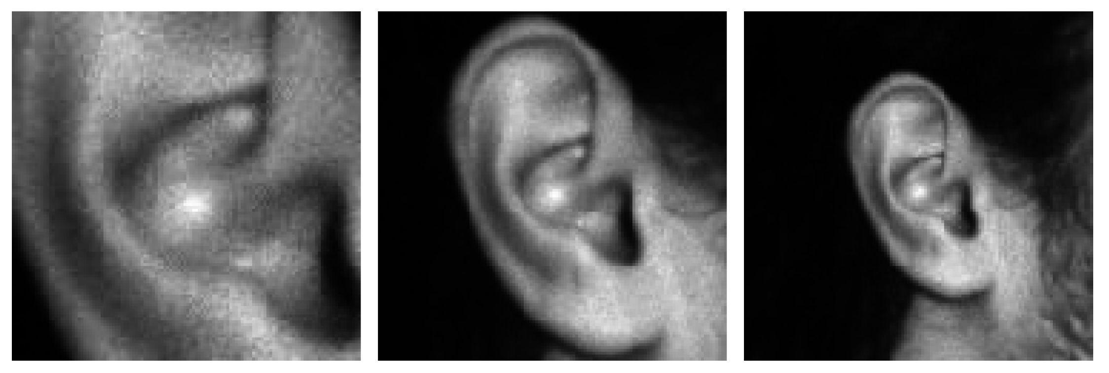
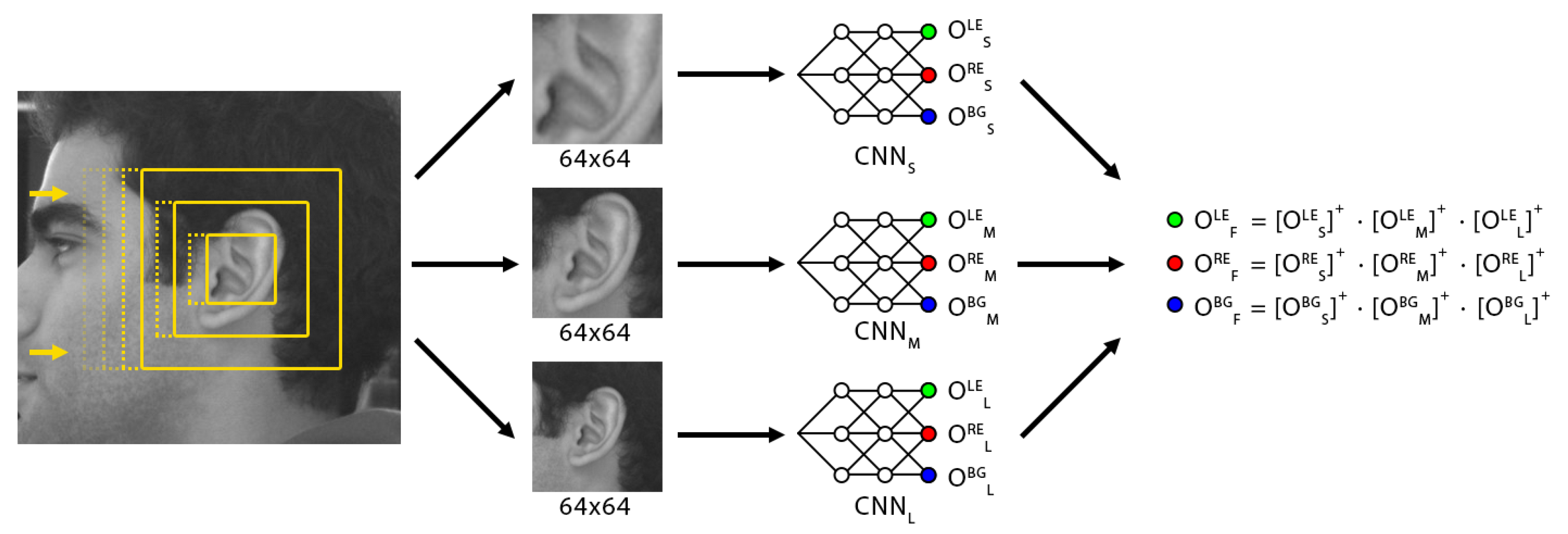
The main idea then is to feed to three neural networks three different images, each one corresponding to the same image region being analyzed but at different cropping scales. Figure 3 depicts the three different scales which are ingested by the triple classifier ensemble. We appropriately label each of the three networks used to analyze these as S, M, and L (for their corresponding size abbreviations).

The purpose of the three scales is mainly to train specialized networks for the specific purposes of (i) recognizing the tubular features of the inner ear, (ii) framing the correct coordinates of the ear, and (iii) inferring ear context within a surrounding head region. Training a network with any single one of these scales would specialize it in that particular data, but the network would be oblivious to other natural image data with similar structure but not really belonging to a true ear, and thus leading it to produce a large number of false positives which would end up affecting the overall detection accuracy. However, the three networks working together as a committee of classifiers produces a much more robust result that is far more resilient against noise, as a true positive hit will require the activation of all three networks, simply by integrating contextual information into the system.

Each of the three neural networks produces three output values, which correspond to the likelihood of each target class having been perceived in that network’s input. We denote the output values as $O_A^K$, where $A\in \{S,M,L\}$ represents the network index denoted by its size, and $K\in \{LE,RE,BG\}$ represents the output class index of each network, for each of the possible detection outcomes. Each of these outputs will lie in the $[-1,+1]$ range as the neural networks have been trained with those ideal values.

To combine the outputs of all three networks as a unified ensemble, we filter each class output with the corresponding values across all three networks, after each one has been linearly rectified. The final outputs of the ensemble are defined by:

$$\begin{array}{cc}\hfill O_F^{LE}& ={\lceil O_S^{LE}\rceil }^{+}·{\lceil O_M^{LE}\rceil }^{+}·{\lceil O_L^{LE}\rceil }^{+}\hfill \end{array}$$

(2)

$$\begin{array}{cc}\hfill O_F^{RE}& ={\lceil O_S^{RE}\rceil }^{+}·{\lceil O_M^{RE}\rceil }^{+}·{\lceil O_L^{RE}\rceil }^{+}\hfill \end{array}$$

(3)

$$\begin{array}{cc}\hfill O_F^{BG}& ={\lceil O_S^{BG}\rceil }^{+}·{\lceil O_M^{BG}\rceil }^{+}·{\lceil O_L^{BG}\rceil }^{+}\hfill \end{array}$$

(4)

where ${\lceil x\rceil }^{+}\equiv max(0,x)$, is a linear rectification operation. By passing through only the positive values of each interim output, we avoid interference from multiple negative values, any of which then has the effect of zeroing the final output. Figure 4 depicts the process visually.

The net effect of this process, then, is to have all three networks work in tandem, where only the regions for which all three networks are in full agreement will survive. Furthermore, the final output will be weighed by the individual network certainty, and thus regions where all three networks have a high likelihood output will outweigh regions where the output distribution is more disparate.

3.4. Training Data

As the system will comprise three individual neural networks, we already know beforehand that the training data will need to be gathered in accordance to the requirements for each of the individual networks.

It was previously discussed that each network will essentially analyze three different crop sizes of each region, so the data for all three can be prepared simultaneously by simply starting with one dataset, and extending it by cropping and scaling accordingly to generate the data for the two other sizes.

Existing image datasets consisting of segmented ear photographs are very scarce and small in volume. Creating sufficiently large amounts of training data, therefore, required a lot of manual labor in image manipulation. The datset UBEAR v1.0 was particularly helpful, as described in Section 3.1, in that it includes for each of its images a ground truth mask. This mask outlines the exact location of the ear in each image, and this aided in cropping out the corresponding bounding boxes for each ear. Not all patches from this dataset could be used, however, as many were extremely blurry and not appropriate for training. In the end, approximately 3000 images were used from this set for training data.

Furthermore, we supplemented the training data with additional samples that were manually cropped from video frames. These originate from the Videos (Train) dataset described in Section 3.1. With this addition, the training dataset now consisted of roughly 4000 images.

To increase the dataset size even more, the data was augmented in two ways: (i) images were randomly modified by adding small translations, rotations and rescales; and (ii) images were horizontally flipped, and the resulting image was assigned to the opposite ear dataset. This artificial augmentation boosted the training data size tenfold. It now consisted of approximately 40,000 images, or 20,000 for each ear.

In order to prepare for the training of our final 3-CNN architecture, we processed the images for each ear side into three separate sets, for each of the 3-CNN scales: S, M, and L. This was done by simply cropping and rescaling each sample appropriately.

The process was repeated for both sides, thus producing six separate image collections for left and right ears, at each of the three scales. Finally, one more background noise dataset was also created, of the same size as the others, and consisting of randomly cropped patches from a large flickr photo database and from non-ear regions of the UBEAR and Videos training sets.

In total, we ended up with seven distinct collections for training purposes, each one consisting of roughly 20,000 images. Figure 5 shows an example of these.

3.5. Network Training

Our final neural network classifier was trained with the three-scale collection described above. Each of the three networks used a 3-class training dataset compiled from left and right ears at the corresponding network scale, and a copy of the background image collection.

The structure of all three networks was exactly the same, and is the one described in Section 3.2. The input consists of a single grayscale channel image resized to a square of size $64\times 64$. The input images are then passed through a pre-processing step which consists of a Spatial Contrastive Normalization (SCN) process, which helps to enhance image edges and redistribute the mean value and data range, something which greatly aids in the training of CNNs.

Each network is trained with its corresponding small, medium or large datasets. A standard SGD approach was used for training, and ran for a duration of approximately 24 iterations until no further improvement could be made on the test-fold of the data. Ideal targets for each of the output labels were assigned in the $\left[-1,+1\right]$ range, where active labels are positive, and inactive labels are negative. This distribution was chosen in this manner (as opposed to the more traditional $\left[0,1\right]$ range) to aid with the 3-CNN inference as explained in Section 3.3.

All datasets are divided into training and testing folds, at an 80% to 20% ratio as per standard machine learning training practices. The final results of training over these two sets are summarized in

Table 5. Final confusion matrix of the training data fold.

Classified As/Real Class	Left Ear	Right Ear	Background	Total in Class	Accuracy (%)
Left Ear	16,040	56	88	16,184	$99.11$
Right Ear	46	16,064	74	16,184	$99.26$
Background	63	194	15,927	16,184	$98.41$
			Total	48,552	$98.93$

and

Table 6. Final confusion matrix of the testing data fold.

Classified As/Real Class	Left Ear	Right Ear	Background	Total in Class	Accuracy (%)
Left Ear	3964	34	49	4047	$97.95$
Right Ear	14	4002	31	4047	$98.89$
Background	8	42	3997	4047	$98.77$
			Total	12,141	$98.54$

.

3.6. Detection

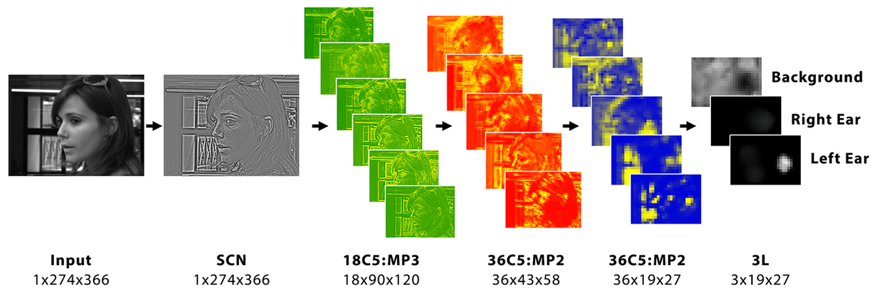
Runtime operation of the network is performed through Shared Map execution of CNNs. This allows for an optimized method of inferring detection predictions from a full image frame in a manner that is much more efficient than the traditional sliding window approach.

The process requires the input image to be first prepared as a multi-scale pyramid. This is simply to be able to detect ears in all possible sizes relative to the image frame, so as to be able to properly carry out the detection, regardless of the subject’s relative distance to the camera.

Each of these pyramid levels will be given to each of the three networks to be analyzed independently. Each network, thus, creates three output maps per level, corresponding to each of the target classes trained, LE, RE, and BG. Figure 6 depicts the shared map execution of one of the networks for a particular pyramid level of size $274\times 366$.

Every pixel in each of these output maps corresponds to that class’ predicted likelihood at a window whose location can be traced back to the input image according to the shared map’s alignment and position configuration. Figure 7 shows how windows can be re-constructed from these shared maps and they correspond precisely to the multiple detections that a traditional sliding window approach would produce, but at a fraction of the computing time.

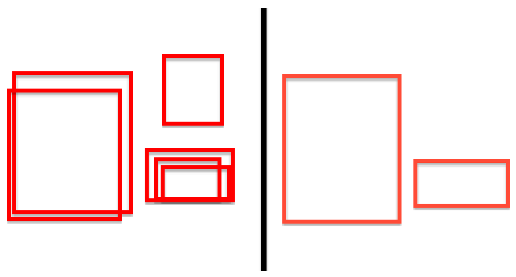
In order to collapse these multiple detections into a single final result, a partitioning algorithm based on Disjoint-set data structures is used. This is very similar to the groupRectangles and partition functions of OpenCV [35], but customized in a few particular ways. This algorithm allows the grouping of similarly positioned and scaled windows as all belonging to a single object detection. Figure 8 shows a diagram of how the grouping algorithm would behave on various sample window clusters.

This is a very common practice taken as a post-processing cleanup procedure in many computer vision tasks. For this particular work, however, a special grouping rule is created in order to weigh the grouping allowance.

For each of the two positive classes, LE and RE, the following procedure is performed:

Every window i has a value assigned to it corresponding to the neural network output prediction value at that window, denoted by $O_i$. This window weighs its own value by squaring itself. Therefore, windows with a low prediction value have their overall importance reduced, whereas windows with a large output value to begin with, maintain their standing in the grouping.

For a potential grouping cluster j composed of N multiple windows, each with a weighed output value $O_i^2$, the final output value $G_j$ for the group is then given by:

$$G_j=\sqrt{\frac{{\sum }_i^N{O}_i^2}{N}}$$

(5)

This corresponds to an RMS of all composing window output values in that cluster. The end result of this is that the process favors those clusters that are composed of windows with large significant confidence outputs, where as windows with low confidence (such as in the case of false positives) end up with a lower value.

As each cluster has a single final numerical value assigned to it corresponding to its overall significance, a thresholding operation can be passed through all final clusters in order to reject those with low confidence.

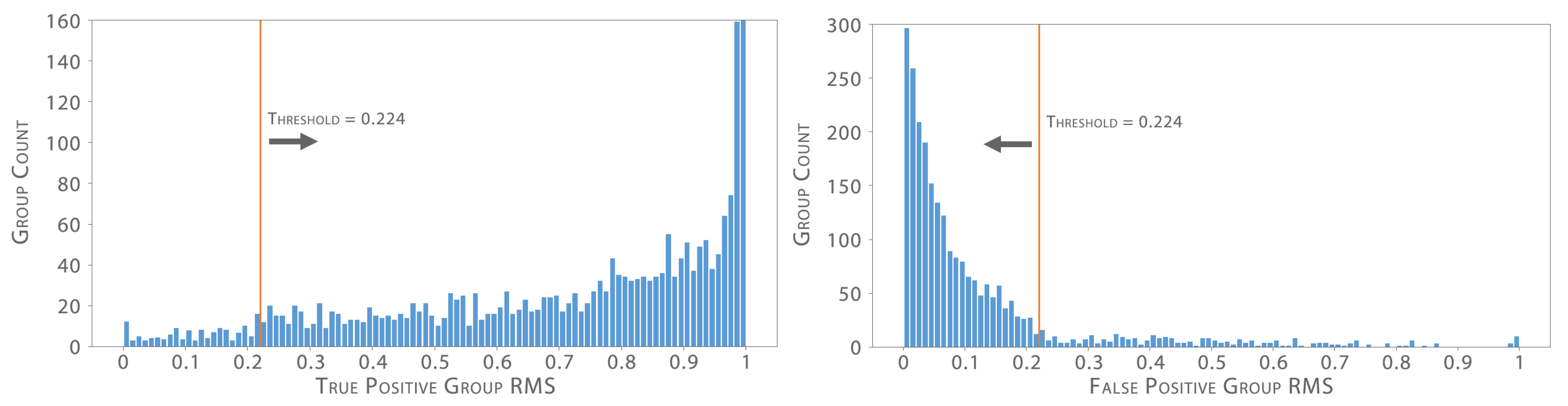
In order to find a suitable threshold value, an experiment was performed over the full UBEAR test dataset. All final clusters generated in this process were then manually classified as either True Positive or False Positive. Figure 9 shows the distribution of True Positive cluster output values and that of clusters classified as False Positives. After analyzing these distributions, it can be seen that the chosen threshold value of 0.224 most optimally separates it, where a balance can be achieved in rejecting the largest majority of false positive hits, while keeping as many true positives as possible above the threshold.

Note that this process, although similar to traditional Non-Maximum Suppression (NMS), has the added advantage of providing a better filtering mechanism of detections that are likely to be false positives. NMS simply clusters boxes together and keeps the box with highest confidence per cluster, regardless of the distribution of confidence values in the remaining boxes. The proposed method, by comparison, takes into account a weighted distribution of all contributing detections in order to make a more informed decision on the filtering, as this method requires all contributing detections in each clustered set to have a higher confidence value.

A summary of this whole process, starting from the inference, continuing through the grouping, and ending in the thresholding operations, is listed in Algorithm 1:

Algorithm 1 The proposed process including steps for inference, grouping, and applying the threshold.

for all$Z\in \left\{PyramidScales\right\}$do     for all$A\in \{L,M,S\}$do         $O_A^{LE},O_A^{RE},O_A^{BG}\leftarrow SharedMap(Imag{e}_Z,Networ{k}_A)$     end for     for all$K\in \{LE,RE,BG\}$do         $O_{F,Z}^K\leftarrow Ensemble(O_S^K,O_M^K,O_L^K)$     end for end for for all$K\in \{LE,RE\}$do     $G^K\leftarrow Group\left(O_{F,Z}^K\right)$     if$G^K>Threshold$then         $Keep\left(G^K\right)$     else         $Discard\left(G^K\right)$     end if end for

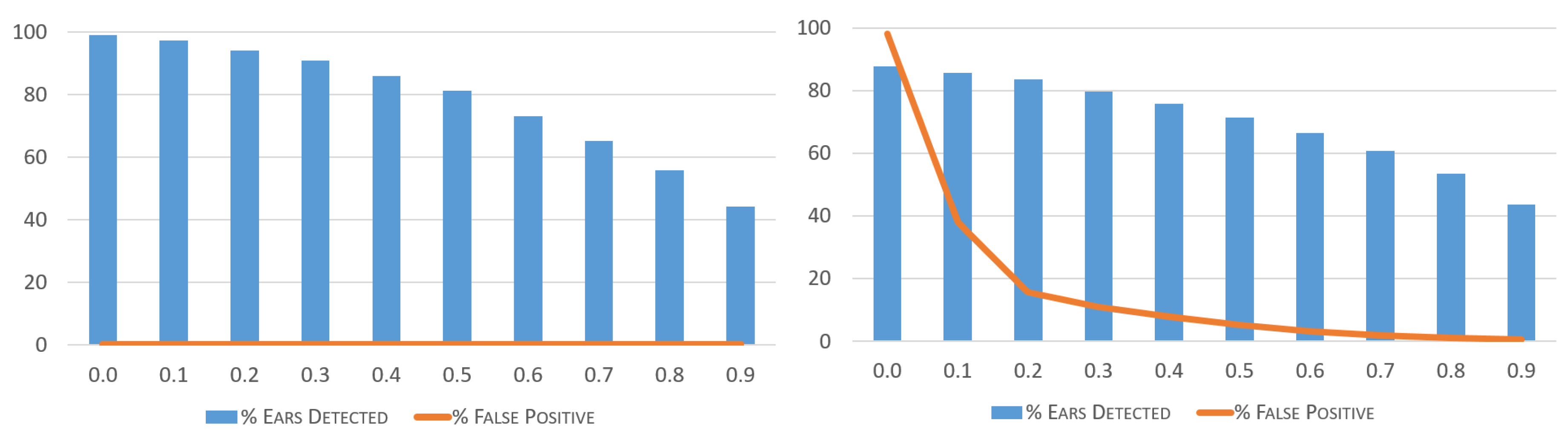
The correct threshold to use should be carefully decided upon depending on the type of data being analyzed. In the case of the AMI database, where images are already prepared as cropped ears, the system detects no False Positives whatsoever, and thus the threshold value decision does not affect the False Positive rate in any way. In this case, a very low (or zero) threshold can be chosen in order to maximize the number of correctly detected ears. This can be seen in the results shown in Figure 10, where the accuracy rate of varying threshold amounts is depicted.

In the case of natural images in non-cooperative environments as with the UBEAR dataset, the effect of false positives is much more important, as can be seen in Figure 10, where small variations in the threshold value lead to a drastic drop in the false positive rate, while not significantly affecting the accuracy of detected ears.

4. Experiments

4.1. Test Methodology

Multiple experiments were conducted with the various datasets in order to evaluate the system’s accuracy in different scenarios. For all tests, the experiment was carried out with the 3-CNN method proposed in this work. To contrast the results, the same tests were also performed with a standard Haar Cascade Classifier trained on similar data as implemented in OpenCV [35], and executed with a similar sliding window configuration while post-processing them with the same window grouping algorithm.

In all cases, the results reported are defined as follows:

• True Positive: Detection groups which successfully enclose the bounding box of an ear within the image.
• False Positive: Detection groups which mis-classify the side of the ear detected, or which erroneously detect noise in the image that does not correspond to an actual ear.
• False Negative: Ears in an image which failed to be detected by the network entirely, or whose final detection group confidence value was below the selected threshold.
• True Negative: This value would usually describe the rate at which non-ear noise is successfully ignored by the classifier. However, in the case of full image frames, this would greatly offset the result bias by greatly increasing the overall classification accuracy needlessly. We avoid recording this on purpose such that the results given represent the true nature of correctly classified ears only.

The performance metrics reported for all cases are the precision which measures the exactness of the classifier; the recall which measures its completeness; and the F1 metric which provides a balance between precision and recall, and is therefore a more objective comparison of the performance of two classifiers. Furthermore, the traditional accuracy rate is also reported, in order to provide a basic performance metric.

4.2. Comparison with State of the Art

Due to varied nature of the state of the art in this field, it is very difficult to make a comparative study on performance of our proposed method with all of the existing methods in the literature. In part, this is due to there not being a standard dataset by which all of these algorithms have be benchmarked, but rather every method so far examined in Section 2.1 tends to use their own private data. Similarly, testing existing methods on the same data we use is difficult as most existing implementations remain private and their source code is not readily available for implementation.

Therefore, we can only contribute to Table 1 with our own accuracy results on datasets such as UND and AMI, which are images of similar qualities as the data used in those studies, consisting of ready made images made for this exact purpose. In the case of closeup cropped images such as AMI, our 3-CNN system reaches an accuracy of 99.0% and an F1 metric of 99.50%. On full frame images, such as UND, where localization also plays a part, our system reaches an accuracy of 95.25% and an F1 metric of 97.57%. Full details on these results are found in Section 4.6.

4.3. Video Analysis

Additionally, we also test the detection accuracy on individual video frames. An experiment was carried out with the Video dataset as described in Section 3.1. The purpose of this test is to ensure that both ears can be correctly classified as either left or right, while working with data of variable head poses.

Results of these tests is presented in

Table 7. Results of testing over the Videos dataset.

		Haar					3-CNN
	Subset Size	Precision (%)	Recall (%)	Accuracy (%)	F1 Score (%)		Precision (%)	Recall (%)	Accuracy (%)	F1 Score (%)
Middle	470	97.60	97.60	95.32	97.60		$99.57$	$99.79$	$99.36$	$99.68$
Upwards	162	100	69.75	69.75	82.18		$95.95$	$91.03$	$87.65$	$93.42$
Downwards	284	98.77	57.09	56.69	72.36		$94.83$	$95.19$	$90.49$	$95.01$
Left Ear	455	97.85	71.21	70.11	82.43		$97.07$	$97.29$	$94.51$	$97.18$
Right Ear	461	98.53	88.57	87.42	93.29		$97.98$	$96.46$	$94.58$	$97.21$
Complete Dataset	916	99.05	80.07	79.45	88.55		97.59	96.95	94.68	97.27

, where it can be seen that our system greatly outperforms Haar in this particular task.

The significance of this test is in the ability to continuously detect the same ear on a moving image sequence, regardless of head orientation. The high detection rate ensures that the ear is consistently detected during the majority of each video’s duration, except for a few odd frames where detection might fail from time to time. However, a few frames later, the ear is found again and detection continues as normal. This result rate would therefore allow for a tracking mechanism to be successfully implemented in such video streams.

4.4. Image Resolution

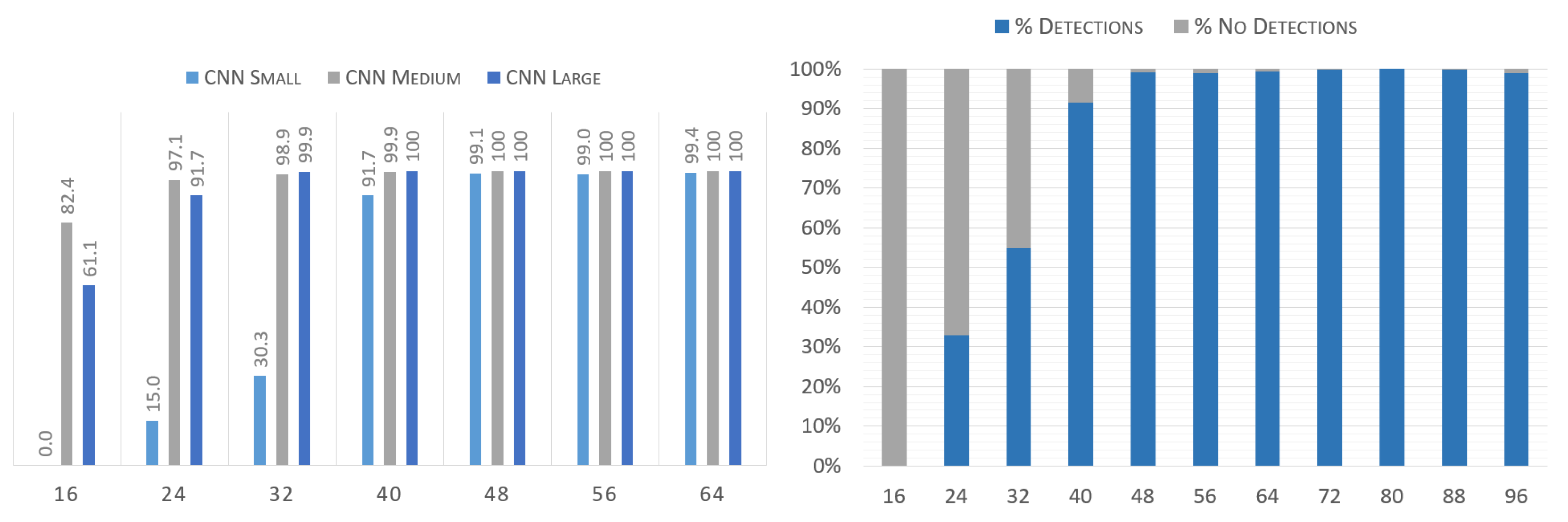
Detecting images of subjects at a great distance from the camera is usually problematic. To quantitatively measure the performance of the system in cases where the relative size of the image is very small, various tests were performed on the AMI dataset with the ears previously resized at different scales, ranging from $16\times 16$ up to $96\times 96$. The results of both the combined 3-CNN system as well as that of the individual S, M, and L CNNs are displayed in Figure 11.

This shows that even ears which are found at scales much lower than the networks’ input size of $64\times 64$ can still be successfully detected, albeit at a lower rate depending on the actual size.

Figure 11, in particular, explains the dropoff in resolving power at smaller scales. The S CNN is the first one to fail at diminishing scales, as could be expected due to the nature of the data this network analyzes. Meanwhile, the other two CNNs continue to detect with sufficient accuracy at even the smallest scales. Arguably, it could be said that a system without the S scale might do better for this particular purpose, as the dropoff exhibited by the S CNN is the main reason behind the 3-CNN difficulty in detecting smaller sized ears. However, the S CNN has been shown before to be essential for noise differentiation, and as such, this side effect is an acceptable tradeoff.

4.5. Non-Cooperative Natural Images

Traditional computer vision approaches usually require the ear to be perfectly aligned, or at the very least in the same plane as the photograph projection, thus imposing restrictions that are very restrictive when analyzing real world imagery. Due to the ability of CNNs to learn multiple representations of the same object, and given the pose variety used in the training data, the final trained system is capable of detecting ears at very different angles with respect to the camera.

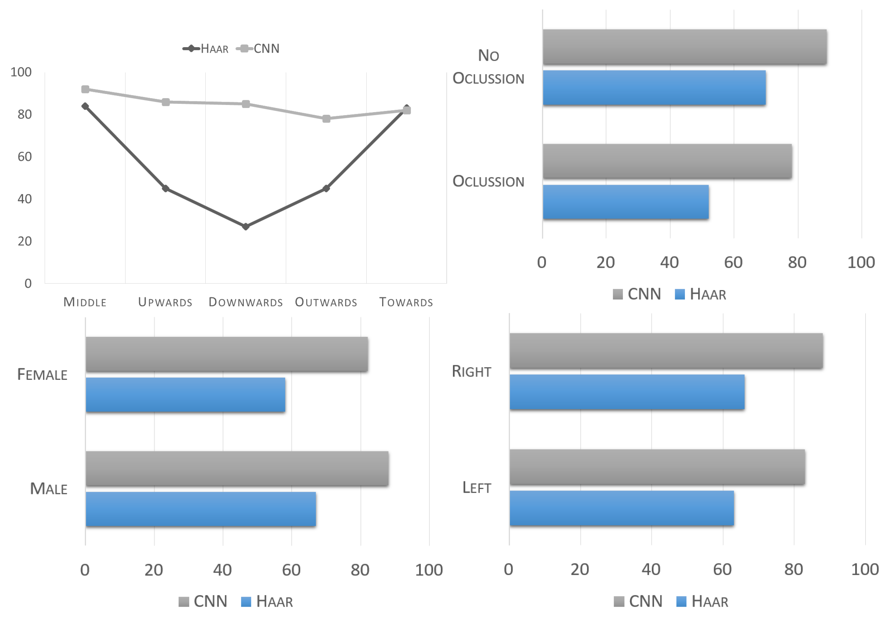
The UBEAR dataset contains labels for each image which facilitates its partitioning according to the relative pose of the subject in relation to the camera. Tests were run over the full dataset and the results were divided according to the angle of the subject’s gaze. These results are depicted in Figure 12 and summarized in

Table 8. Detection performance of our 3-CNN system vs. Haar on the different data folds of the UBEAR dataset.

		Haar					3-CNN
	Subset Size	Precision (%)	Recall (%)	Accuracy (%)	F1 Score (%)		Precision (%)	Recall (%)	Accuracy (%)	F1 Score (%)
Middle	1392	95.90	74.31	72.03	83.74		$89.89$	$93.92$	$84.95$	$91.86$
Upwards	813	85.87	30.42	28.97	44.93		$87.47$	$84.94$	$75.73$	$86.19$
Downwards	784	88.65	16.23	15.90	27.44		$85.68$	$84.57$	$74.09$	$85.12$
Outwards	789	89.96	30.34	29.35	45.37		$85.92$	$71.26$	$63.81$	$77.91$
Towards	829	95.10	73.24	70.57	82.75		$79.70$	$84.40$	$69.47$	$81.99$
Male	3403	94.17	51.58	49.99	66.65		$86.10$	$87.84$	$76.93$	$86.96$
Female	1204	91.06	42.47	40.77	57.92		$86.99$	$77.83$	$69.71$	$82.15$
Left Ear	2289	93.49	47.33	45.82	62.84		$83.64$	$83.11$	$71.48$	$83.37$
Right Ear	2318	93.42	51.07	49.30	66.04		$88.97$	$87.32$	$78.79$	$88.14$
Occlusion	1491	89.70	36.49	35.03	51.88		$85.01$	$71.63$	$63.60$	$77.75$
No Occlusion	3116	94.70	55.24	53.59	69.78		$86.79$	$91.53$	$80.34$	$89.10$
Complete Dataset	4607	93.45	49.22	47.58	64.48		86.31	85.23	75.08	85.77

.

The common trend of our 3-CNN outperforming Haar continues to be seen here. However, the real significance behind these results is that Haar, not unlike most traditional computer vision approaches, is highly dependent on viewpoint, and its performance largely drops off as the angle varies from the more normal “Middle” and “Towards” angles. Meanwhile, our 3-CNN system maintains a very similar and stable performance rating regardless of the angle at which the ear is presented.

Further UBEAR labels can be used to split the data into additional folds, such as ear sidedness. As expected, the system works mostly the same for either left or right side ears. The small differences in the results might just be due to a random variation in the images, and not to a real side preference of the classifier.

Finally, we tested the system on images which were marked to have occlusion against those that did not. Occlusion is not a defined label in the UBEAR dataset, therefore, for this study, we manually defined this data fold based on a subjective decision of which images could be considered as occluded. This is because degrees of occlusion can vary from merely a few small strands of hair or a small earring, to very large accessories or full sections of hair covering well over half of the ear. The final occlusion threshold decision was made to mark only those ears which had their outline covered at least 25%. This resulted in approximately one third of the images to be marked as occluded.

Not surprisingly, the 3-CNN system performs better when no occlusion is present. However, it is worth noting that even when analyzing occluded ears, the 3-CNN system outperforms Haar when it analyzes clearly visible, and non-occluded ears.

Furthermore, analyzing the literature of existing ear detection systems, such as those described in Table 1, it is obvious that most of the systems which seemingly have very high reported accuracy rates on clearly defined ear images, would drastically fail when the ear is occluded in any way—especially those systems which rely on shape analysis and detection of the tubular or helix properties of an ear.

A final study was performed on gender sensitivity of the detector. The classifiers are not necessarily sensitive to the different shapes of male and female ears. However, a visible disparity can be seen, simply due to the fact that female ears are far more likely to be occluded by longer hair or more prevalent accessories such as large earrings. Thus, gender sensitivity results closely resemble those of occlusion sensitivity.

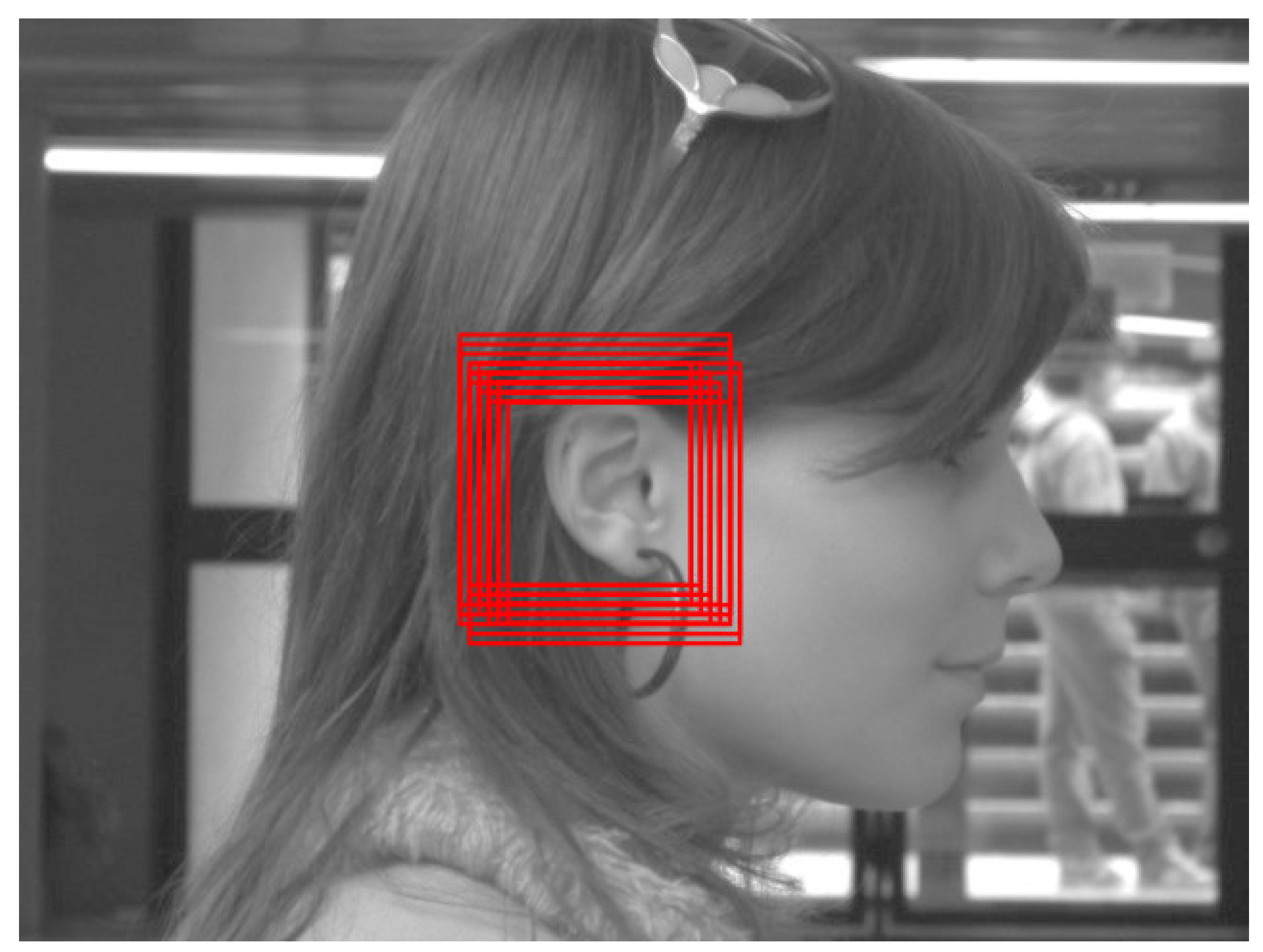
Figure 13 shows a few selected samples of the 3-CNN and its detection in particularly challenging images, due to either occlusion or extreme viewpoint perspectives.

4.6. Summary

To conclude,

Table 9. Summary of the total results over all four datasets contrasting the Haar and 3-CNN algorithms.

Dataset	Algorithm		Positive	Negative	Precision (%)	Recall (%)	Accuracy (%)	F1 Score (%)
UND [32,33]	3-CNN	Positive	461	20	95.84	99.35	95.25	97.57
		Negative	3	0
	Haar	Positive	270	7	97.47	58.44	57.57	73.07
		Negative	192	0
Videos	3-CNN	Positive	890	22	97.59	96.95	94.68	97.27
		Negative	28	0
	Haar	Positive	727	7	99.05	80.07	77.47	87.31
		Negative	181	0
AMI [31]	3-CNN	Positive	693	0	100.00	99.00	99.00	99.50
		Negative	7	0
	Haar	Positive	382	7	98.20	55.12	54.57	70.61
		Negative	311	0
UBEAR [34]	3-CNN	Positive	3814	605	86.31	85.23	75.08	85.77
		Negative	661	0
	Haar	Positive	2227	156	93.45	49.22	47.58	64.48
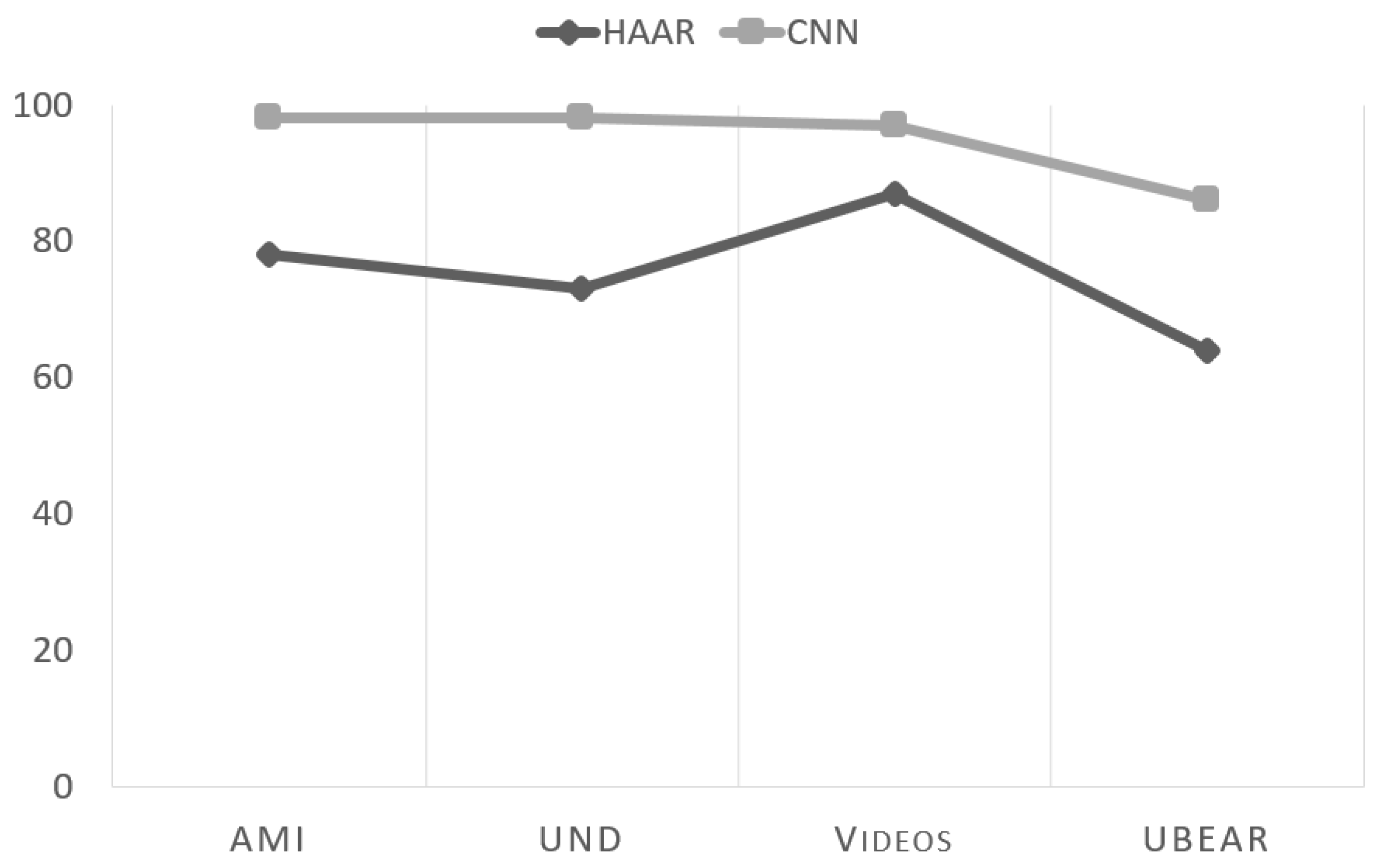
		Negative	2298	0

lists a summary of all total results across all four datasets while comparing our 3-CNN system with the well known Haar Cascade Classifier algorithm.

As can be seen, the CNN based system always outperforms the Haar algorithms in all sets, by an amount ranging between 10% to 29% in the F1 metric. This is particularly so in the UBEAR dataset, since the Haar classifier is incapable of modelling the higher variety of internal representations required to properly classify images in that dataset.

Figure 14 shows a summary of these results. It is important to remark that that our proposed system has stable performance figures across the first three datasets, all of which consist of perfect purpose-made ear photography. The results only slightly drop when presented with natural images due to the challenges already described. This is in contrast to the Haar classifier, which has wildly disparate results, demonstrating the large dependency of this system on the particular conditions of one dataset or another.

5. Conclusions

We propose a new technique based on CNNs to carry out ear detection on natural images. As opposed to traditional computer vision approaches that are based on hand-crafted features, Convolutional neural networks perform image and shape perception, which is far more robust against variable perspective, occlusion and illumination conditions. These difficult conditions are very common in natural images, compared to synthetic photographs taken in strictly controlled photographic and illumination conditions.

All previously proposed systems usually fail in one important way or another. Some require the ear to be properly aligned. Others require the full ear to be visible. Most commonly, they are highly sensitive to illumination and require images shot in the exact same conditions as the training data, or they may even fail when the images are not fully in focus or when the relative size of the ear in the image is not sufficiently large.

Up to now, we have not seen a robust all-encompassing system capable of detecting ears under all possible conditions in natural images, and we are glad to introduce this new alternative. Granted, our system still has some important failures which we must address in future versions of the system, primarily to decrease the false positive rate, which would allow decreasing the threshold and thus improve the overall performance. However, the results so far are very encouraging, and having such a robust detector is the first important step towards building an ear recognition system, something which obviously is a future line of research to be conducted presently.

Further future lines of research include the implementation of this system in an even more optimized manner in order to deploy it on low power mobile or embedded devices for practical biometric applications.

Finally, it is important to note that although this work was aimed mainly towards ear detection, it presents an end-to-end object recognition framework which can be adapted very similarly to other computer vision tasks requiring a comparable type of classification executed over natural imagery for real-time detection and tracking. Convolutional neural networks have been shown time and time again to be extremely powerful image classifiers, especially when they are used as ensemble systems, and this work has presented one more way in which they can be applied to this kind of task.