Wind Energy Generation Assessment at Specific Sites in a Peninsula in Malaysia Based on Reliability Indices


1
Center for Advanced Power and Energy Research, Faculty of Engineering, University Putra Malaysia, Selangor 43400, Malaysia
2
Advanced Lightning, Power and Energy Research, Faculty of Engineering, University Putra Malaysia, Selangor 43400, Malaysia
3
Faculty of Electronics Information Engineering, Huaiyin Institute of Technology, Huai’an 223003, China
*
Author to whom correspondence should be addressed.
Processes 2019, 7(7), 399; https://doi.org/10.3390/pr7070399
Submission received: 12 April 2019
/
Revised: 18 May 2019
/
Accepted: 22 May 2019
/
Published: 27 June 2019
(This article belongs to the Special Issue Advances in Theoretical and Computational Energy Optimization Processes)
Abstract
:This paper presents a statistical analysis of wind speed data that can be extremely useful for installing a wind generation as a stand-alone system. The main objective is to define the wind power capacity’s contribution to the adequacy of generation systems for the purpose of selecting wind farm locations at specific sites in Malaysia. The combined Sequential Monte Carlo simulation (SMCS) technique and the Weibull distribution models are employed to demonstrate the impact of wind power in power system reliability. To study this, the Roy Billinton Test System (RBTS) is considered and tested using wind data from two sites in Peninsular Malaysia, Mersing and Kuala Terengganu, and one site, Kudat, in Sabah. The results showed that Mersing and Kudat were best suitable for wind sites. In addition, the reliability indices are compared prior to the addition of the two wind farms to the considered RBTS system. The results reveal that the reliability indices are slightly improved for the RBTS system with wind power generation from both the potential sites.
1. Introduction
Recent environmental impacts and the depletion of fossil fuel reserves are the main concerns that have stimulated the integration of renewable energy power plants using solar power, wind power, biomass, biogas, etc. as alternative sources of electrical generation. This has inspired global concerns in energy balance, sustainability, security, and environmental preservation [1].
Wind energy is non-depletable, free, environmentally friendly, and almost available globally [2]. It is intermittent, though very reliable from a long-term energy policy viewpoint [3]. In the measure of adequacy, wind energy is regarded as a better choice compared with other energies.
Electric power systems continue to witness the penetration of high-level wind power into the system as a global phenomenon [4], due to the problems associated with power system planning and operation. This makes the assessment of wind power generation system capacities, and their impacts on reliability in the system by appropriate planning, in line with their power utilization and environmental benefits. Thus, high penetration of intermittent wind energy resources into the electric power system requires the need to investigate the system reliability while adding a large amount of varying wind power generation to the system [5].
Owing to the industrial development and growth in the economy, an increase in the demand for electricity is one of the major challenges faced by both developed and developing countries like Malaysia. This has precipitated the Malaysian electrical utility to integrate wind generation based renewable energy into the grid. Many studies have been carried out by researchers to identify the potential location of wind energy systems in Malaysia. This process has been encouraged by both public and private institutions, with the aim of producing green energy [6,7]. In addition, the extraction of power from wind energy is optimized, even in location with average wind speed, by the proper design of wind turbine models that can effectively trap power due to the advancement in technologies [8].
In general, Malaysia experiences low wind speeds, but some particular regions experience strong winds in specific periods of the year [9]. Locations like Mersing experience higher wind speed variations throughout the year, with average wind speeds ranging from 2 m/s to 5 m/s [10]. According to the literature, the wind in Malaysia could be able to generate a great quantity of electric energy despite its lower average wind speeds, especially at the eastern coastal areas or its remote islands [11]. Researchers in [12] applied the Weibull function to investigate the characteristics of wind speed and subsequently evaluated the wind energy generation potential at Chuping and Kangar in Perlis, Malaysia. Furthermore, small capacity wind turbine plants (5–100 kW) have been installed by the Ministry of Rural and Regional development in Sabah and Sarawak [11]. Researchers in [13] stated that ten units of wind turbines with three different rated powers (6, 10, and 15 kW) were used in energy calculation for the area in the north part of Kudat. As the wind turbine units are principally dependent on wind velocity and location, wind speed forecast is essential for siting a new wind generating turbine in a prospective location [14], as the study in Kudat location reveals. Moreover, another study was performed by a research group of the University of Malaysia (UM) using the Weibull distribution function for the analyses of wind energy potential at the sites in Kudat and Labuan in the Sabah region in Malaysia [6]. The outcome of this research demonstrated that Kudat and Labuan are suitable for sitting small-scale wind generating units [15].
The question to ask here is whether it is probable to harness small-scale wind generating units at selected locations in Malaysia for the purpose of electricity generation. So far, studies on wind power characteristics in Malaysia are limited and wind speed depends on geographical and meteorological factors. This study discusses the effect of potential wind power from various locations in Malaysia for adequately reliable power systems. Analysis of the wind speed data characteristics and wind power potential assessment at three given locations in Malaysia was done. The main objective of the paper is to examine the capacity contribution of wind power in generating system adequacy and its impact on generation system reliability. The Sequential Monte Carlo simulation (SMCS) technique and Weibull models are employed to demonstrate the impact of wind power in power system reliability. Also, the results presented in the paper could serve as preliminary data for the establishment of a wind energy map for Malaysia.
This paper is structured in six sections. The introduction includes a brief introduction of the concept for the wind energy potential in Malaysia. The next section describes related work adapted to enable estimation of the wind power potential of the region. Section 3 shows the fundamental reliability indices evaluated in this work, which are used by assessment policy makers to exploit the wind power potential of the region. Section 4 describes the wind speed data analysis at specific sites in Malaysia. Section 5 shows the obtained results of the simulation in the case study, which are also discussed. Finally, Section 6 summarizes the main conclusions of the study.
2. Related Work
2.1. Weibull Distribution for the Estimation of Wind Power and Energy Density
The Weibull distribution is the most well recognized mathematical description of wind speed frequency distribution. The value of the scale parameter c of the Weibull distribution is close to the mean wind speed in actual wind speed data, and because of that, the Weibull distribution is a reasonable fit for the data. Consequently, using the two parameters (shape parameter k and scale parameter c), the Weibull distribution can be used with acceptable accuracy to present the wind speed frequency distribution and to predict wind power output from wind energy conversion system (WECS) [16].
Many numerical methods are employed to estimate the values of the shape parameter k and scale c. The Empirical Method (EM) is used in this paper for calculating the Weibull parameters. The EM can be calculated by employing mean wind speed and the standard deviation, where the Weibull parameters c and k are given by the following equations [17].
where is standard deviation, is the mean wind speed, is the gamma function, and k can be determined easily from the values of and , which are computed from the wind speed data set provided with the following formulation [18].
where is the mean wind speed (m/s), n is the number of measured data, is wind speed of the observed data in the form of time series of wind speed (m/s), and is standard deviation. Once k is obtained from the solution of the above numerical expression (1), the scale factor c can be calculated by the above Equation (2).
Wind power density is a beneficial way of evaluating wind source availability at a potential height. It indicates the quantity of energy that can be used for conversion by a wind turbine [19]. The power that is available in the wind flowing at mean speed, , through a wind rotor blade with sweep area, An (m2), at any particular site can be projected as
The monthly or annual mean wind power density per unit area of any site on the basis of a Weibull probability density function can be displayed in [20] as follows:
where p(v) is the wind power (Watts), PD(w) is the mean wind power density (Watts/m2), ρ is the air density at the site (1.225 kg/m3), A is the sweep area of the rotor blades (m2), and (x) is the gamma function.
The extractible mean energy density over a time period (T) is calculated as
where the time period (T) is expressed a daily, monthly or annual.
2.2. Estimation of Wind Turbine Output Power and Capacity Factor
The performance of how a wind machine located in a site performs can be assessed as mean power output Pe,ave over a specific time frame and capacity factor, Cf, of the wind machine. Pe,ave determines the total energy production and total income, whereas Cf is a ratio of the mean power output to the rated electrical power Prated of the chosen wind turbine model [21]. Depending on the Weibull distribution parameters, the Pe,ave and capacity factor Cf of a wind machine are computed according to the following equations.
where Vc is cut-in wind speed and Vr is the rated wind speed of the wind turbine generator (WTG). For an economical and viable investment in wind power, it is advisable that the capacity factor should exceed 25% and be maintained in the range of 25–45% [22].
2.3. Extrapolation of Wind Speed at Different Heights
Indirect wind speed estimation methods consist of measuring wind speed at a lower height and applying an extrapolation model to estimate the wind speed characterization at different elevations. The most commonly used model is the power law [23].
Wind speed increases significantly with the height above ground level, depending on the roughness of the terrain. Therefore, correct wind speed measurements must consider the hub height (H) for the WTG and the roughness of the terrain of the wind site. If measurements are difficult at high elevations, the standard wind speed height extrapolation formula, as in the power law Equation (9) [24], can be used to estimate wind speed at high elevations by using wind speed measured at a lower reference elevation, typically 10 m [25].
where v is the wind speed estimated at desired height, H; vo is the wind speed reference hub height Ho, and (n) is the ground surface friction coefficient. The exponent (n) is dependent on factors such as surface roughness and atmospheric stability. Numerically, it ranges from (0.05–0.5) [26]. The normal value of ground surface for every station is approximated 1/7 or 0.143, as suggested by [27] for neutral stability conditions.
3. Reliability Assessment for Generation Systems
3.1. Fundamental Reliability Indices
The Load and generation models are conjoined to produce the risk model of the system. Indices that evaluate system reliability and adequacy can be used to forecast the reliability of the power generating system.
The fundamental reliability indices evaluated in this work are adapted to enable the estimation of the reliability level of the power generating systems, comprised of Loss of Load Frequency (LOLF), Loss of Energy Expectation (LOEE), Loss of Load Duration (LOLD), and Loss of Load Expectation (LOLE).
At present, LOLE represents the reliability index of the electrical power systems used in many countries [3]. The standard level of LOLE is one-day-in ten years or less. This does not mean a full day of shortages once every ten years; rather, it refers to the total accumulated time of shortages, which should not exceed one day in ten years. Therefore, the level of LOLE in this study is used as a reliability index of the generation systems.
The combined Sequential Monte Carlo simulation (SMCS) method (or the Monte Carlo simulation method cooperate with Frequency and Duration method) in [28] enables accurate evaluation of reliability indices. To accurately evaluate the reliability assessment for the overall reliability of generating systems adequacy containing wind energy, an SMCS method was used alongside the Weibull distribution model to generate and repeat the wind speed. The Roy Billinton Test System (RBTS) is an essential reliability test system produced by the University of Saskatchewan (Canada) for educational and research purposes. The RBTS has 11 conventional generating units, each having a power capacity ranging of around 5–40 MW, with an installed capacity of 240 MW and a peak load of 185 MW. Figure 1 shows the single line diagram for the RBTS, and the detailed reliability data for the generating units in the test system are shown in Appendix A. The load model is generally represented as chronological Load Duration Curve (LDC), which is used along with different search techniques. The LDC will generate values for each hour, so there will be 8736 individual values recorded for each year. The chronological LDC hourly load model shown in Figure 2 was utilized, and the system peak load is 185 MW. Besides the traditional generators, the wind farm was comprised of 53 identical WTG units with a rated power of 35 kW, each of which was considered in the current study. A peak load of 1% penetrated wind energy in the RBTS system, which has a peak load of 185 MW.
3.2. Proposed Methodology
The basic simulation procedures for applying the SMCS with the Weibull model in calculating reliability indices for the electrical power generating systems with wind energy penetration are based on the following steps.
Step 1: The generation of the yearly synthetic wind power time series employs a Weibull model, as follows:
- Set the Weibull distribution parameters k and c.
- Generate a uniformly distributed random number U between (0,1).
- Determined the artificial wind speed v with Equation (10).
- Set the WTG’s Vci, Vr, and Vco wind speeds.
- Determine the constants A, Bx, and Cx with the equations below.
- Calculate the WTG output power using Equation (11),where ws = wind speed (m/s), Vci = WTG cut-in speed (m/s), Vco = WTG cut-out speed (m/s), Vr = WTG rated speed (m/s), and Pr = WTG rated power output (MW). The constants A, Bx, and Cx have previously been calculated by [3].
Step 2: Create the total available capacity generation by a combination of the synthetic generated wind power time series with a conventional chronological generating system model by employing SMCS, as follows:
- Define the maximum number of years (N) to be simulated and set the simulation time (h), (usually one year) to run with SMCS.
- Generate uniform random numbers for the operation cycle (up-down-up) for each of the conventional units in the system by using the unit’s annual MTTR (mean time to repair) and λ (failure rate) values.
- The component’s sequential state transition processes within the time of all components are then added to create the sequential system state.
- Define the system capacity by aggregating the available capacities of all system components by combining the operating cycles of generating units and the operating cycles with the WTG available hourly wind at a given load level.
- Superimpose the available system capacity curve on the sequential hourly load curve to obtain the available system margin. A positive margin denotes sufficient system generation to meet the system load whereas a negative margin suggests system load shedding.
- The reliability indices for a number of sample years (N) can be obtained using Equations (12)–(18).where i = 1, 2… N, N = number of years simulated, Ф(sji) = index function analogous to jth occurrence within the year i, j = 1, 2…, nj(s), nj(s) is the number of system state occurrences of (sj) in the year i, sj = ssuccess ᴜ sfailure is the set of all possible states (sj) (i.e., the state-space), and the content of two subspaces ssucess of the success state and sfailure of the failure states.where ΔPj×T is the amount of curtailing energy in the failed state (sji).Δλj, is the sum of the transition rates between sj and all the ssuccess states attained from sj in one transition.
- If (N) is equal to the maximum number of years, stop the simulation; otherwise, set (N = N + 1), (h = 0), then return to move 2 and repeat the attempt.
Step 3: Evaluate and update the outcome of the test function for the reliability indices evaluation. The above procedure is detailed in the form of flowchart, as represented in Figure 3.
4. Wind Speed Data Analysis at Specific Sites in Malaysia
To estimate the possible potential wind energy site in Malaysia, the analysis, correlation, and prediction of wind data from the location need to be done. It has been often recommended in the literature that making use of the wind data available from meteorological stations increases the vicinity of the proposed candidate site by preliminary estimates of the wind resource potential of the site. Meteorological data that are recorded for long periods need to be extrapolated to obtain an estimation of the wind profile of the site. In this study, wind speed data from Mersing, Kudat, and Kuala Terengganu have been statistically analyzed to propose the wind energy characteristics for these sites. The data for this study were gathered from the Malaysia Meteorological Department (MMD). The data recorded comprise three years of hourly mean surface wind speeds from 2013 to 2015 at three locations in Malaysia. The mean of the wind speed form the simulated process for each hour is calculated based on Weibull parameters. The hourly mean wind speed is then used in the sequential simulation process. Figure 4 shows the locations of MMD stations in Peninsular Malaysia. This map was drawn by using the Arc Graphical Information System (AGIS) software and depicts the strength of the wind speed distribution in Mersing, Kudat, and Kuala Terengganu. The area that showed the highest wind speed value is in red and orange, while other areas show moderate wind speeds. Table 1 presents a description of the selected regions in Malaysia, which consist of the latitude, longitude, and elevation of the anemometer.
4.1. Estimation of Average Wind Speed with Different Height
In this study, the scale parameter (c) of Weibull distribution was applied to test the generated wind speed data from the Weibull model at the Mersing, Kudat, and Kuala Terengganu sites. The monthly average wind speed data for the three sites within the three year period, with a scale parameter, are presented in Figure 5. It is clear from the figures that for the entire three years of the wind speed data and scale parameter c of the Weibull distribution they showed similar variations during one year.
Wind speed is typically measured at standard heights, such as 10 m, but there is the need to obtain wind speed values at a high level in cases where the electricity is generated by the mean power of a wind turbine [29]. The wind power law has been acknowledged to be a beneficial tool and is frequently employed in assessing the wind power where wind speed data at different elevations must be adjusted to a standard height before use. In this study, the exponent n of the power law is set to 0.143 for the Kudat and Kuala Terengganu sites, as suggested by [13]. Meanwhile, for the Mersing site, the exponent n of the power law is set to 0.5, according to the nature of the ground. Wind data taken from the MMD station were measured at a level height of 43.6 m for Mersing. However, wind data of the Kudat and Kuala Terengganu sites require the data to be converted at a height of 10 m above hub height, because the wind turbine always runs at elevations above 10 m height.
Figure 6 shows both monthly and annual mean wind speeds at the sites (Mersing, Kudat, and Kuala Terengganu) for the average years of 2013–2015; these results were extrapolated to a different height. In this study, the wind speed was extrapolated for various heights (mean wind observation station, 60 m, and 100 m) in the wind observation stations at Kudat, Kuala Terengganu, and Mersing (extrapolated). The obtained results are presented in Table 2.
All the tabulated values reveal that the wind speed increases with an increase in elevation. For Mersing, the annual average wind speed was 2.82 m/s, 3.31 m/s, and 4.27 m/s at wind observation station elevations of 60 m, and 100 m, respectively. Furthermore, the annual average wind speeds in Kudat and Kuala Terengganu were 2.45 m/s, 3.68 m/s, and 3.95 m/s; and 2.03 m/s, 2.89 m/s, and 3.10 m/s at wind observation station elevations of 60 m, and 100 m, respectively.
4.2. Estimation of Wind Power Density and Energy Density at Different Heights
The observed wind speed data at the station were converted to 100 m height wind speed data using Equation (9), and then the converted data were used to determine the wind potential. The scale c and shape k Weibull parameters were estimated using the EM. The wind power and energy density were measured, respectively, by Equations (5) and (6) at heights of (43.6 m) and (100 m) in Mersing, as shown in Table 3. The rest of the calculations for wind power and energy density at heights of 3.5 and 100 m and 5.2 and 100 m in Kudat and Kuala Terengganu, respectively, can be found in Appendix B.
From Table 3, it is observed that the maximum power density from the actual wind speed of Mersing, Kudat, and Kuala Terengganu was found to be 52 W/m2, 19 W/m2, and 20 W/m2, respectively. However, the maximum power density of Mersing, Kudat, and Kuala Terengganu, when the actual wind speed data was converted to 100 m height, was calculated to be 180 W/m2, 80 W/m2, and 72 W/m2, respectively. Here, it is evident that the Mersing site has a higher mean monthly power density compared to Kudat and Kala Terengganu under various heights.
The annual mean power density of Mersing, Kudat, and Kuala Terengganu varies between 84.59 W/m2, 79.28 W/m2, and 33.36 W/m2 at a height of 100 m. The annual power density is also less than 100 W/m2 for all the locations, and, therefore, these locations can be categorized as a class 1 wind energy resource. This wind energy resource class, in general, is inappropriate for large-scale wind turbine applications. Nevertheless, the generation of small-scale wind energy at a turbine height of 100 m [6] is viable. However, for small-scale applications, and in the long-term with the development of wind turbine technology, the use of wind energy continues to hold great promise.
4.3. Estimation of the Suitable Wind Turbine Units at Malaysia Sites
The selection of the wind turbine should be made with a rated wind speed that corresponds to the maximum energy wind speed in order to maximize energy output. For the annual energy output, the selected wind turbine will have the maximum capacity factor, defined by the ratio of the actual power generated to the rated power output [30]. The average power output values, Pe,ave, and Cf, are crucial performance factors of the wind energy conversion system (WECS).
The technical data of six differently sized wind turbines are summarized in Table 4. The summarized information in Table 4 is obtained from [13,19]. The cut-in wind speed, or the speed at which the turbine commences power production, is 2.7 m/s for four of the six turbines, while for the other two turbines, the cut-in wind speed values are 2 and 3.5 m/s, respectively. The cut-out wind speed of 25 m/s applies to all the turbines. Table 4 represents the information pertaining to the rated speed, rated output power, hub height, and rotor diameter of the wind turbines analyzed.
Depending on the turbine’s characteristics in Table 4, and the Weibull parameters derived from applying EM using the Matlab toolbox, the electrical output of the wind turbines can be made available by using the formulation earlier defined in Equation (7).
Knowing the output power of the wind turbines, it is then possible to obtain a computation of the average output power value of each wind turbine. As the capacity factor of a wind turbine is the ratio of its average output power to its rated power, the energy output data are employed in calculating the capacity factor of the wind turbines, which are of sizes 20, 22, 25, 35, 50, and 100 kW. A comparison of the capacity factors computed for various wind turbines at different heights is presented in Figure 7.
From Figure 7, it can be seen that the capacity factor goes up as the hub height increases. Moreover, the capacity factor increases for wind turbines of a size of 35 kW. In Mersing, the maximum capacity factor is achieved as about 23.66% for the Endurance America model of the G-3120 kW wind turbine, whereas in Kuala Terengganu, the lowest capacity factor is achieved as approximately 7.82% for the Endurance America model of the G-3120 kW wind turbine. Kudat, with about 19.21%, ranks second in terms of capacity factors compared to the regions.
The G-3120 (35 kW) wind turbine has the highest capacity factors of 23.66%, 19.21%, and 7.82%, at suggested heights of 100 m for Mersing, Kudat, and Kuala Terengganu, respectively, among the models considered. Therefore, the reliability analysis was carried out only for Mersing and Kudat, which have high capacity factors, whereas Kuala Terengganu was not considered as it has low capacity factors.
5. Results and Discussion
In this section, the reliability indices evaluation of generating systems for wind power generation using a sequential Monte Carlo simulation (SMCS) is presented. In addition, the strategies for wind farm operation at Malaysian sites (Mersing and Kudat) are presented and compared by assessing the reliability of wind energy generation when adding to the RBTS test system [31].
5.1. Case Studies
As reported in the literature, two wind generating stations suggested at the specific sites in Malaysia, Mersing and Kudatas, have low wind speed and thus require small-scale rated power wind turbines of around 35 kW for installation in two selected locations for reliability analysis.
Reliability analysis using the simulation technique suggested in this paper is applied to the RBTS, which contains the WECS. The hourly wind data obtained from the two locations—Mersing and Kudat—atre used for studying the hourly wind speed of the Weibull model considered for the simulation. Then, the Weibull parameters c and the k are obtained by the empirical method. The obtained values were used to generate hourly wind speed data for deducing the available wind power from the wind turbine generators (WTG) chosen for both of the sites for reliability assessment.
The values of c are around 4.88 and 4.46 m/s, and the values of k for wind speed distribution are 2.25 and 1.84 for Mersing and Kudat at the proposed height of 100 m, respectively; these values were obtained by simulation. The WTG unit that is selected for installation in the farm has the following specifications: Vci = 3.5 m/s, Vr = 8 m/s, and Vco = 25 m/s, and the rated power output of every WTG unit is Pr = 35 kW [19]. Figure 8 and Figure 9 show the simulated output power with 35 kW for each WTG in the sampling year, and the simulation of the farm with output power is 1.85 MW for 53 WTG units in Mersing.
The RBTS was simulated for 600 trials using the SMCS method. The simulation proceeded in chronological order from one hour to the next, repeatedly, using yearly samples until the specified convergence criteria were met. Figure 10 shows the available capacity for the power system containing wind power generation from the wind farm in Mersing during the simulated process for yearly samples and the superimposition of the available capacity with the chronological load model. It can be seen from this state of the system that the available capacity of the power generating system is not sufficient to meet the load demands. Thus, there are some intersections that are seen in the diagram. Figure 11 represents the reliability indices for simulation with (600) sampling years. The values of LOLE, the amount of the LOEE, and the frequency of losing a load during the simulation process are depicted in Figure 11 for wind power in the Mersing site.
5.2. Calculated Reliability Indices for RBTS Including Wind Power Generation
To evaluate the contribution of wind energy to the overall reliability of the generating systems, Table 5 compares the reliability indices before and after adding the 53 WTGs and 106 WTGs to the conventional units of RBTS. The results obtained were compared with the results obtained from the SMCS method reported in [32]. The simulation process was terminated after a set number of samples (600 times) had been achieved. The results show that the reliability indices demonstrate a distinguished and slightly improved reliability of RBTS, including wind power from both locations (Mersing and Kudat) by the addition of 1.85 MW and 3.71 MW from the proposed wind farms. The LOLE and LOEE indices are typically employed to gauge the extent of benefits in assessing the wind energy of generating systems. Therefore, after adding the wind generating 1.85 MW to the system, the LOLE index was reduced to 1.115 and 1.131 h/year for Mersing and Kudat, respectively, when compared with the results from the base case, which shows the reliability assessment of the power generation system. Additionally, after adding the wind generating 3.71 MW to the system, the LOLE index wass reduced to 0.987 and 1.128 h/year for Mersing and Kudat, respectively, when compared with the results from the base case, which shows the reliability assessment of the power generation system.
Further, it can be observed that this study was done with a small percentage of peak load reduction at around 1% and a small number of wind turbines, to demonstrate the primary effect of wind energy penetration from selected locations in Malaysia in the reliability of the generation system for the RBTS.
6. Conclusions
In this paper, analyses of the wind speed data characteristics and wind power potential assessment at three given locations in Malaysia were done. In addition, this study tests the effects of the potential wind power from different locations. An SMCS technique is used to show the effects of wind energy for the RBTS test system by a set of reliability indices. The results reveal that the wind power connected to the RBTS test system is only from two locations in Malaysia. Further, the reliability indices are compared prior to and after the addition of the two farms to the considered system. The results show that the reliability indices are slightly improved for RBTS, including wind power from both locations, as suggested. Moreover, the wind resources at specific sites in Malaysia are more suitable for small-scale standalone energy conversion systems and could also be hybrid energy systems.
Recommendations for future studies include extending the statistical analysis model used for different sites in Malaysia to include more relevant factors for wind farms and evaluating their impact on wind power potential for these sites, such as wind speeds at the installation site, types of wind turbine offshore and onshore, and numbers of wind turbines installed, according to the size of the farm.
Author Contributions
This work was part of the Ph.D. research carried out by A.A.K. The research is supervised by N.I.A.W. and A.N.A. The project administration and funding acquisition by University Putra Malaysia.
Funding
The authors are grateful for financial support from the University Putra Malaysia (UPM), Malaysia, under Grant No. GP-IPB-9630000.
Conflicts of Interest
The authors declare no conflict of interest.
Appendix A.

Table A1.
The RBTS generating unit ratings and reliability data.
| Units No. | Unit Size (MW) | FOR | MTTF (Hours) | MTTR (Hours) |
|---|---|---|---|---|
| 1 | 5 | 0.01 | 4380 | 45 |
| 2 | 5 | 0.01 | 4380 | 45 |
| 3 | 10 | 0.02 | 2190 | 45 |
| 4 | 20 | 0.02 | 3650 | 55 |
| 5 | 20 | 0.02 | 3650 | 55 |
| 6 | 20 | 0.02 | 3650 | 55 |
| 7 | 20 | 0.02 | 3650 | 55 |
| 8 | 20 | 0.03 | 1752 | 45 |
| 9 | 40 | 0.02 | 2920 | 60 |
| 10 | 40 | 0.03 | 1460 | 45 |
| 11 | 40 | 0.03 | 1460 | 45 |
Forced outage rate (FOR); Mean time to failure (MTTF); Mean time to repair (MTTR).
Appendix B.
Table A2.
Wind power and energy density characteristics at heights of 3.5 m and 100 m in Kudat.
| A height of 3.5 m | A height of 100 m | |||||||||||
|---|---|---|---|---|---|---|---|---|---|---|---|---|
| Months/Year | ⊽ | k | c | PD (w/m2) | Hours | ED (kWh/m2) | ⊽ | k | c | PD (w/m2) | Hours | ED (kWh/m2) |
| January | 2.65 | 3.77 | 2.931 | 14.347 | 747 | 10.717 | 4.28 | 3.77 | 4.734 | 60.450 | 747 | 45.156 |
| February | 2.94 | 4.00 | 3.244 | 19.217 | 675 | 12.972 | 4.75 | 4.00 | 5.239 | 80.946 | 675 | 54.639 |
| March | 2.84 | 3.55 | 3.158 | 18.213 | 747 | 13.605 | 4.59 | 3.55 | 5.100 | 76.709 | 747 | 57.301 |
| April | 2.31 | 2.87 | 2.594 | 10.905 | 723 | 7.884 | 3.73 | 2.87 | 4.190 | 45.957 | 723 | 33.227 |
| May | 2.07 | 2.48 | 2.339 | 8.682 | 747 | 6.485 | 3.35 | 2.48 | 3.777 | 36.555 | 747 | 27.307 |
| June | 2.05 | 1.99 | 2.314 | 10.142 | 723 | 7.333 | 3.31 | 1.99 | 3.738 | 42.753 | 723 | 30.911 |
| July | 2.66 | 2.43 | 3.004 | 18.648 | 747 | 13.930 | 4.30 | 2.43 | 4.851 | 78.528 | 747 | 58.660 |
| August | 2.27 | 2.12 | 2.562 | 12.922 | 747 | 9.653 | 3.66 | 2.12 | 4.137 | 54.406 | 747 | 40.641 |
| September | 2.39 | 2.16 | 2.698 | 14.835 | 723 | 10.725 | 3.86 | 2.16 | 4.356 | 62.433 | 723 | 45.139 |
| October | 2.74 | 2.86 | 3.077 | 17.015 | 747 | 12.710 | 4.43 | 2.86 | 4.969 | 76.777 | 747 | 57.353 |
| November | 2.05 | 2.80 | 2.303 | 7.723 | 723 | 5.584 | 3.31 | 2.80 | 3.719 | 32.524 | 723 | 23.515 |
| December | 2.43 | 3.27 | 2.708 | 11.772 | 747 | 8.794 | 3.92 | 3.27 | 4.373 | 49.574 | 747 | 37.032 |
| Annual | 2.45 | 1.84 | 2.759 | 18.819 | - | 13.738 | 3.95 | 1.84 | 4.456 | 79.284 | - | 57.877 |
Table A3.
Wind power and energy density characteristics at height of 5.2 m and 100 m in Kuala Terengganu.
Table A3.
Wind power and energy density characteristics at height of 5.2 m and 100 m in Kuala Terengganu.
| A Height of 5.2 m | A Height of 100 m | |||||||||||
|---|---|---|---|---|---|---|---|---|---|---|---|---|
| Months/Year | ⊽ | k | c | PD (w/m2) | Hours | ED (kWh/m2) | ⊽ | k | c | PD (w/m2) | Hours | ED (kWh/m2) |
| January | 2.6097 | 3.24 | 2.912 | 14.685 | 747 | 10.969 | 3.98 | 3.24 | 4.443 | 52.157 | 747 | 38.961 |
| February | 2.3543 | 3.10 | 2.632 | 11.020 | 675 | 7.439 | 3.59 | 3.10 | 4.017 | 39.177 | 675 | 26.445 |
| March | 2.0300 | 2.54 | 2.287 | 7.991 | 747 | 5.969 | 3.10 | 2.54 | 3.490 | 28.396 | 747 | 21.212 |
| April | 1.9203 | 2.63 | 2.161 | 6.601 | 723 | 4.772 | 2.93 | 2.63 | 3.298 | 23.463 | 723 | 16.964 |
| May | 1.9381 | 3.16 | 2.165 | 6.089 | 747 | 4.548 | 2.96 | 3.16 | 3.303 | 21.622 | 747 | 16.152 |
| June | 1.7760 | 2.68 | 1.997 | 5.154 | 723 | 3.726 | 2.71 | 2.68 | 3.048 | 18.324 | 723 | 13.248 |
| July | 1.7277 | 3.14 | 1.930 | 4.324 | 747 | 3.230 | 2.64 | 3.14 | 2.946 | 15.378 | 747 | 11.487 |
| August | 1.8242 | 3.61 | 2.024 | 4.774 | 747 | 3.566 | 2.78 | 3.61 | 3.088 | 16.954 | 747 | 12.664 |
| September | 1.7642 | 3.16 | 1.971 | 4.594 | 723 | 3.322 | 2.69 | 3.16 | 3.007 | 16.314 | 723 | 11.795 |
| October | 1.7993 | 2.81 | 2.020 | 5.202 | 747 | 3.886 | 2.75 | 2.81 | 3.083 | 18.496 | 747 | 13.816 |
| November | 1.8165 | 2.87 | 2.038 | 5.288 | 723 | 3.823 | 2.77 | 2.87 | 3.110 | 18.793 | 723 | 13.587 |
| December | 2.8554 | 2.88 | 3.203 | 20.496 | 747 | 15.310 | 4.36 | 2.88 | 4.887 | 72.799 | 747 | 54.381 |
| Annual | 2.0338 | 2.09 | 2.293 | 9.390 | - | 6.854 | 3.10 | 2.09 | 3.499 | 33.366 | - | 24.356 |
References
- Ouammi, A.; Dagdougui, H.; Sacile, R.; Mimet, A. Monthly and seasonal of wind energy characteristics at four monitored locationals in Liguria region (Italy). Renew. Sustain. Energy Rev. 2010, 14, 1959–1968. [Google Scholar] [CrossRef]
- Chaiamarit, K.; Nuchprayoon, S. Modeling of renewable energy resources for generation reliability evaluation. Renew. Sustain. Energy Rev. 2013, 26, 34–41. [Google Scholar] [CrossRef]
- Shi, S.; Lo, K.L. An Overview of Wind Energy Development and Associated Power System Reliability Evaluation Methods. In Proceedings of the 2013 48th International Universities Power Engineering Conference (UPEC), Dublin, Ireland, 2–5 September 2013; pp. 1–6.
- Benidris, M.; Mitra, J. Composite Power System Reliability Assessment Using Maximum Capacity Flow and Directed Binary Particle Swarm Optimization. In Proceedings of the IEEE Conference, Manhattan, KS, USA, 22–24 September 2013; pp. 1–6. [Google Scholar]
- Padma, L.M.; Harshavardham, R.P.; Janardhana, N.P. Generation Reliability Evaluation of Wind Energy Penetrated Power System. In Proceedings of the International Conference on High Performance Computing and Applications (ICHPCA), Odisha, India, 22–24 December 2014; pp. 1–4. [Google Scholar]
- Islam, M.R.; Saidur, R.; Rahim, N.A. Assessment of wind energy potentiality at Kudat and Labuan, Malaysia using Weibull distribution function. Energy 2011, 36, 985–992. [Google Scholar] [CrossRef]
- Taylor, P.; Khatib, T.; Sopian, K.; Ibrahim, M.Z. Assessment of electricity generation by wind power in nine costal sites in Malaysia. Int. J. Ambient Energy 2013, 37–41. [Google Scholar] [CrossRef]
- Gebrelibanos, K.G. Feasibility Study of Small Scale Standalone Wind Turbine for Urban Area: Case Study: KTH Main Campus; KTH School of Industrial Engineering and Management, Energy Technology EGI: Stockholm, Sweden, 2013. [Google Scholar]
- Siti, M.R.S.; Norizah, M.; Syafrudin, M. The Evaluation of Wind Energy Potential in Peninsular Malaysia. Int. J. Chem. Environ. Eng. 2011, 2, 284–291. [Google Scholar]
- Kadhem, A.A.; Abdul, W.N.I.; Aris, I.; Jasni, J.; Abdalla, A.N. Advanced Wind Speed Prediction Model Based on Combination of Weibull Distribution and Artificial Neural Network. Energies 2017, 10, 1744. [Google Scholar] [CrossRef]
- Borhanazad, H.; Mekhilef, S.; Saidur, R.; Boroumandjazi, G. Potential application of renewable energy for rural electrification in Malaysia. Renew. Energy 2013, 59, 210–219. [Google Scholar] [CrossRef]
- Irwanto, M.; Gomesh, N.; Mamat, M.R.; Yusoff, Y.M. Assessment of wind power generation potential in Perlis, Malaysia. Renew. Sustain. Energy Rev. 2014, 38, 296–308. [Google Scholar] [CrossRef]
- Albani, A.; Ibrahim, M.Z.; Yong, K.H. Wind Energy Investigation in Northern Part of Kudat, Malaysia. Int. J. Eng. Appl. Sci. 2013, 2, 14–22. [Google Scholar]
- Goh, H.H.; Lee, S.W.; Chua, Q.S.; Teo, K.T.K. Wind energy assessment considering wind speed correlation in Malaysia. Renew. Sustain. Energy Rev. 2016, 54, 1389–1400. [Google Scholar] [CrossRef] [Green Version]
- Hwang, G.H.; Lin, N.S.; Ching, K.B.; Wei, L.S. Wind Farm Allocation In Malaysia Based On Multi-Criteria Decision Making Method. In Proceedings of the National Postgraduate Conference (NPC), Seri Iskandar, Malaysia, 19–20 September 2011; pp. 1–6. [Google Scholar]
- Chang, T.P. Performance comparison of six numerical methods in estimating Weibull parameters for wind energy application. Appl. Energy 2011, 88, 272–282. [Google Scholar] [CrossRef]
- Kaoga, D.K.; Serge, D.Y.; Raidandi, D.; Djongyang, N. Performance Assessment of Two-parameter Weibull Distribution Methods for Wind Energy Applications in the District of Maroua in Cameroon. Int. J. Sci. Basic Appl. Res. 2014, 17, 39–59. [Google Scholar]
- Kidmo, D.K.; Danwe, R.; Doka, S.Y.; Djongyang, N. Statistical analysis of wind speed distribution based on six Weibull Methods for wind power evaluation in Garoua, Cameroon. Rev. Des. Energ. Renouv. 2015, 18, 105–125. [Google Scholar]
- Adaramola, M.S.; Oyewola, O.M.; Ohunakin, O.S.; Akinnawonu, O.O. Performance evaluation of wind turbines for energy generation in Niger. Sustain. Energy Technol. Assess. 2014, 6, 75–85. [Google Scholar] [CrossRef]
- Ohunakin, O.S.; Adaramola, M.S.; Oyewola, O.M. Wind energy evaluation for electricity generation using WECS in seven selected locations in Nigeria. Appl. Energy 2011, 88, 3197–3206. [Google Scholar] [CrossRef]
- Oyedepo, S.O.; Adaramola, M.S.; Paul, S.S. Analysis of wind speed data and wind energy potential in three selected locations in south-east Nigeria. Int. J. Energy Environ. Eng. 2012, 3, 1–11. [Google Scholar] [CrossRef]
- Anurag, C.; Saini, R.P. Statistical Analysis of Wind Speed Data Using Weibull Distribution Parameters. In Proceedings of the 1st International Conference on Non-Conventional Energy (ICONCE 2014), Kalyani, India, 16–17 January 2014; pp. 160–163. [Google Scholar]
- Molina-García, A.; Fernández-Guillamón, A.; Gómez-Lázaro, E.; Honrubia-Escribano, A.; Bueso, M.C. Vertical Wind Profile Characterization and Identification of Patterns Based on a Shape Clustering Algorithm; IEEE: New York, NY, USA, 2019; Volume 7, pp. 30890–30904. [Google Scholar]
- Ahmed, A.S. Wind energy as a potential generation source at Ras Benas, Egypt. Renew. Sustain. Energy Rev. 2010, 14, 2167–2173. [Google Scholar] [CrossRef]
- Hussain, M.Z.; Roy, D.K.; Khan, S.; Sharma, P.K.; Talukdar, R. Wind Energy Potential at Different Cities of Assam Using Statistical Models. Int. J. Adv. Res. Innov. 2018, 6, 38–43. [Google Scholar]
- Ayodele, T.R.; Ogunjuyigbe, A.S.O.; Amusan, T.O. Wind power utilization assessment and economic analysis of wind turbines across fifteen locations in the six geographical zones of Nigeria. J. Clean. Prod. 2016, 129, 341–349. [Google Scholar] [CrossRef]
- Chandel, S.S.; Ramasamy, P.; Murthy, K.S.R. Wind power potential assessment of 12 locations in western Himalayan region of India. Renew. Sustain. Energy Rev. 2014, 39, 530–545. [Google Scholar] [CrossRef]
- Shi, S. Operation and Assessment of Wind Energy on Power System Reliability Evaluation. Ph.D. Thesis, Department of Electronic and Electrical Engineering, University of Strathclyde, Glasgow, Scotland, 2014. [Google Scholar]
- Dursun, B.; Alboyaci, B. An Evaluation of Wind Energy Characteristics for Four Different Locations in Balikesir. Energy Sour. Part A: Recovery Util. Environ. Eff. 2011, 33, 1086–1103. [Google Scholar] [CrossRef]
- Ayodele, T.R.; Jimoh, A.A.; Munda, J.L.; AgeeWind, J.T. distribution and capacity factor estimation for wind turbines in the coastal region of South Africa. Energy Convers Manag. 2012, 64, 614–625. [Google Scholar] [CrossRef]
- Heshmati, A.; Najafi, H.R.; Aghaebrahimi, M.R.; Mehdizadeh, M. Wind Farm Modeling For Reliability Assessment from the Viewpoint of Interconnected Systems. Electr. Power Compon. Syst. 2012, 40, 257–272. [Google Scholar] [CrossRef]
- Kadhem, A.A.; Abdul Wahab, N.I.; Aris, I.; Jasni, J.; Abdalla, A.N. Computational techniques for assessing the reliability and sustainability of electrical power systems: A review. Renew. Sustain. Energy Rev. 2017, 80, 1175–1186. [Google Scholar] [CrossRef] [Green Version]
Figure 1.
Single line diagrams of the Roy Billinton Test System (RBTS).

Figure 2.
Chronological hourly load (Load Duration Curve (LDC)) model for the RBTS.

Figure 3.
Flow chart showing reliability assessment for a generation system including wind generating sources.
Figure 3.
Flow chart showing reliability assessment for a generation system including wind generating sources.

Figure 4.
Wind speed distribution maps for station sites used in this study in Malaysia.
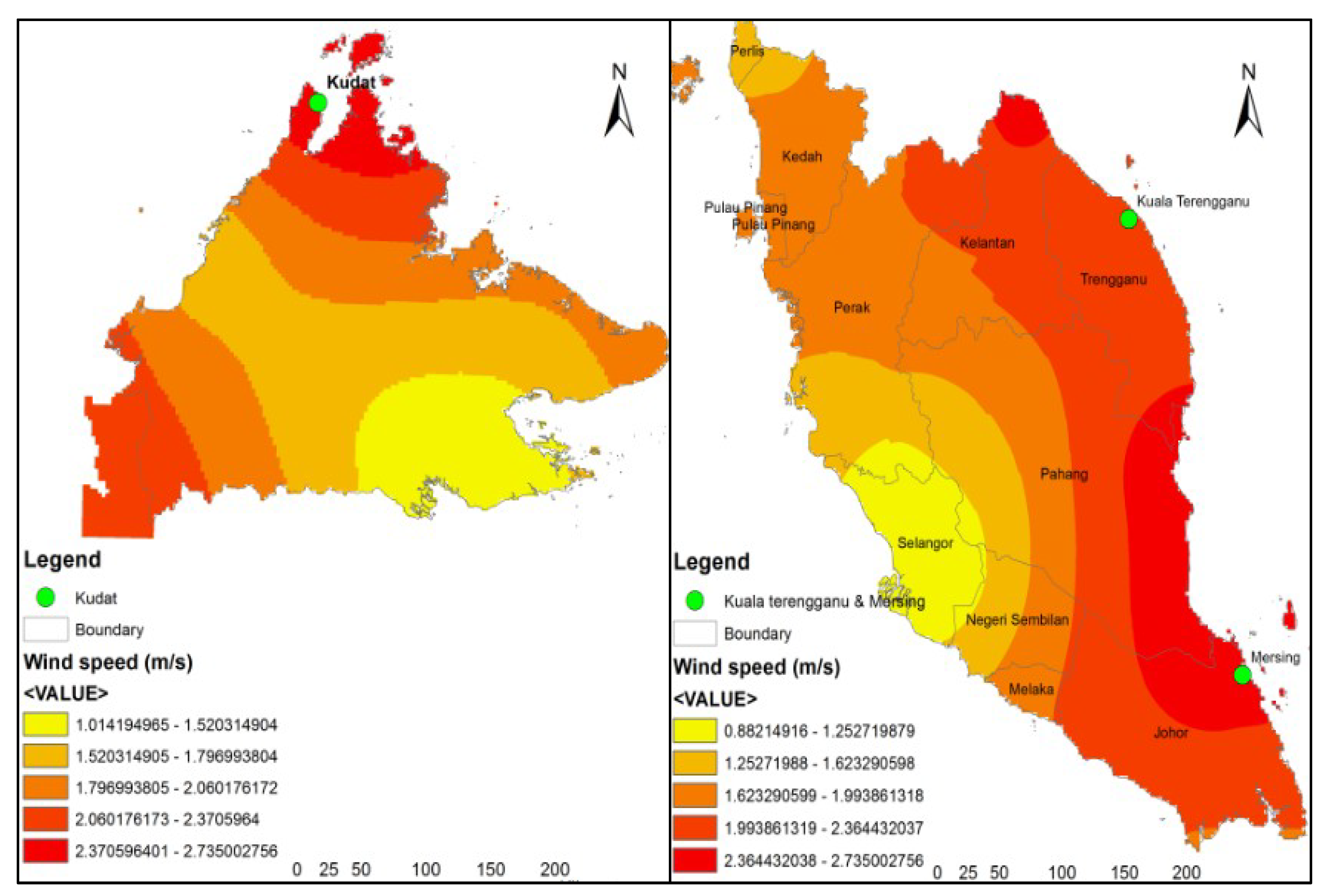
Figure 5.
Comparison between monthly mean wind speed data and the scale parameter (c) over 3 years period at sites (a) Mersing, (b) Kudat, and (c) Kuala Terengganu.
Figure 5.
Comparison between monthly mean wind speed data and the scale parameter (c) over 3 years period at sites (a) Mersing, (b) Kudat, and (c) Kuala Terengganu.
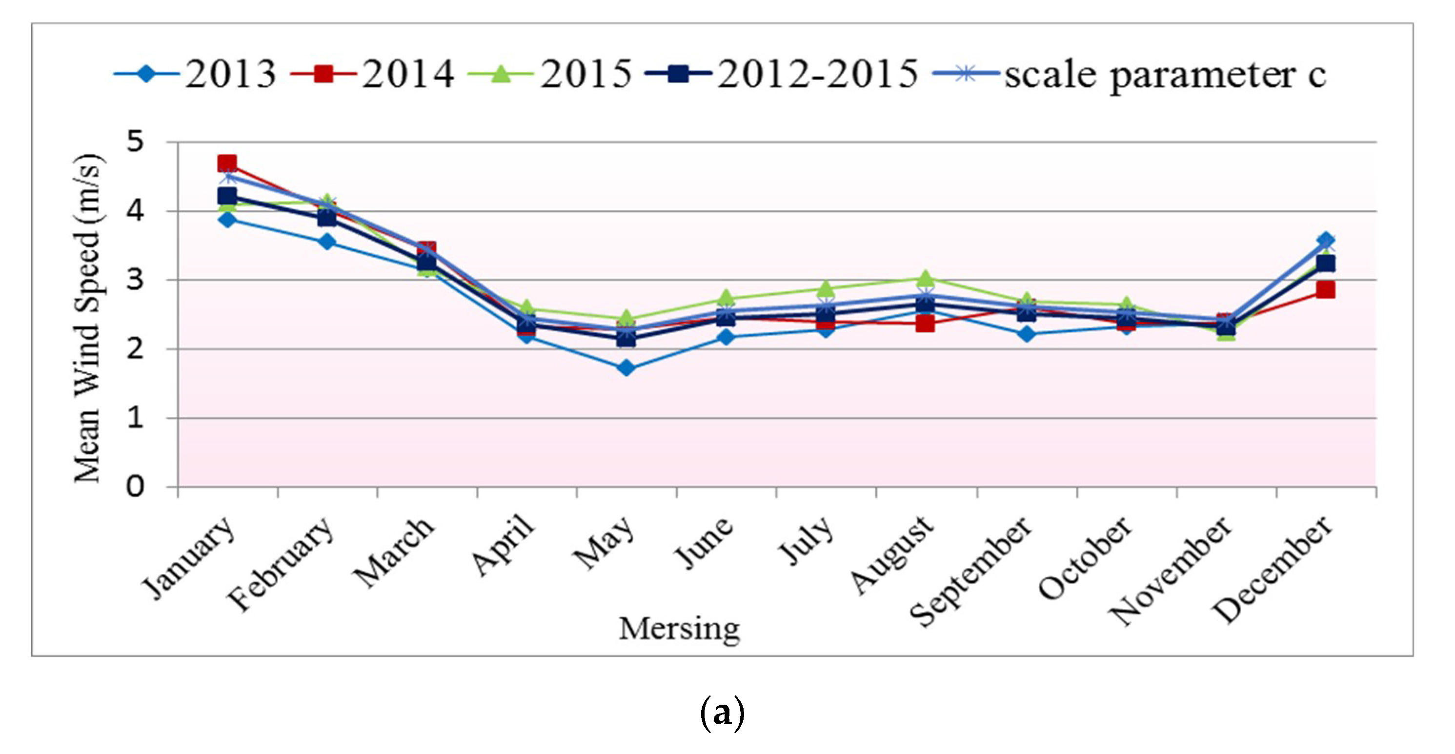
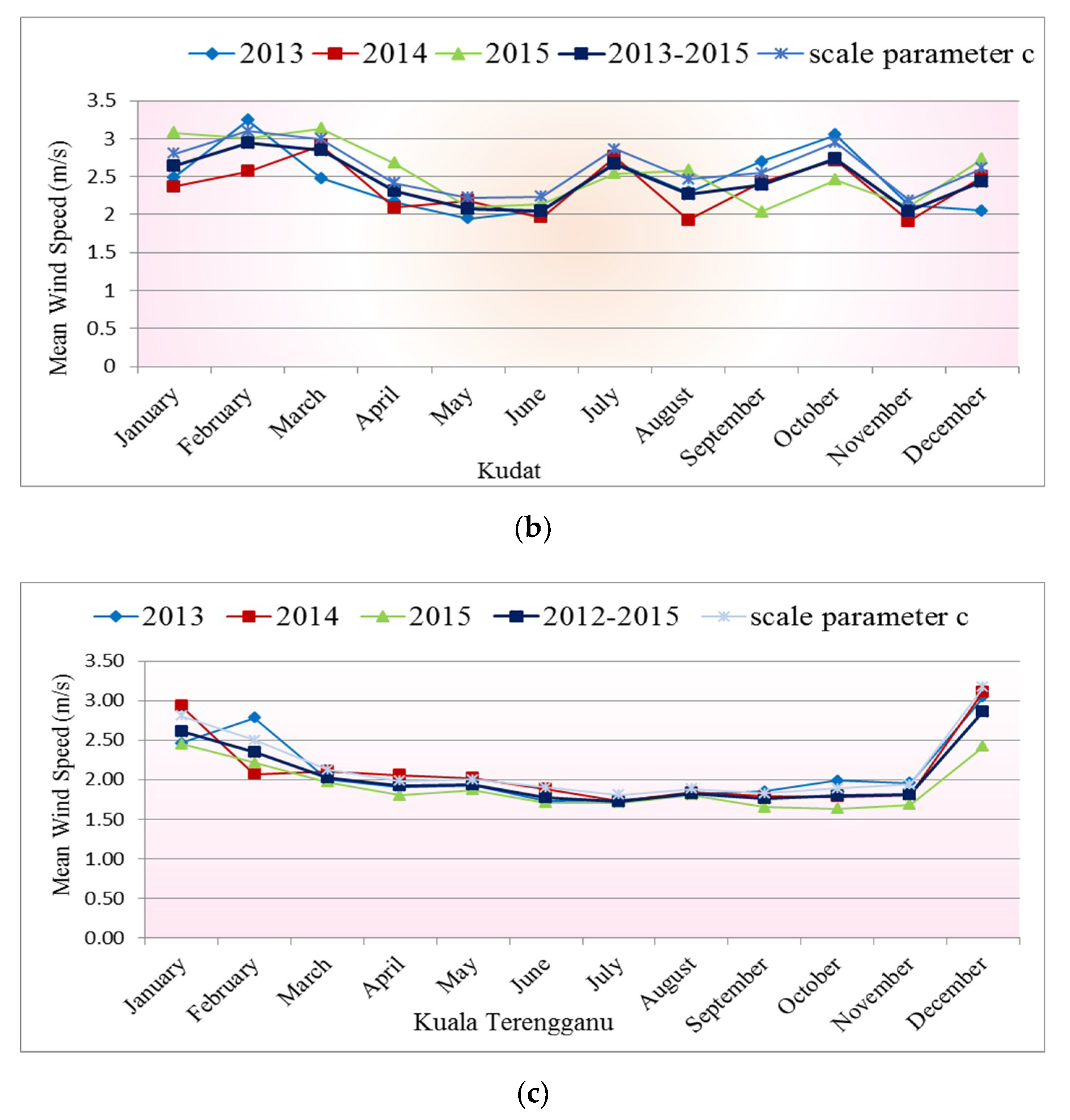
Figure 6.
Monthly and annual mean wind speeds at sites (a) Mersing, (b) Kudat, and (c) Kuala Terengganu.
Figure 6.
Monthly and annual mean wind speeds at sites (a) Mersing, (b) Kudat, and (c) Kuala Terengganu.
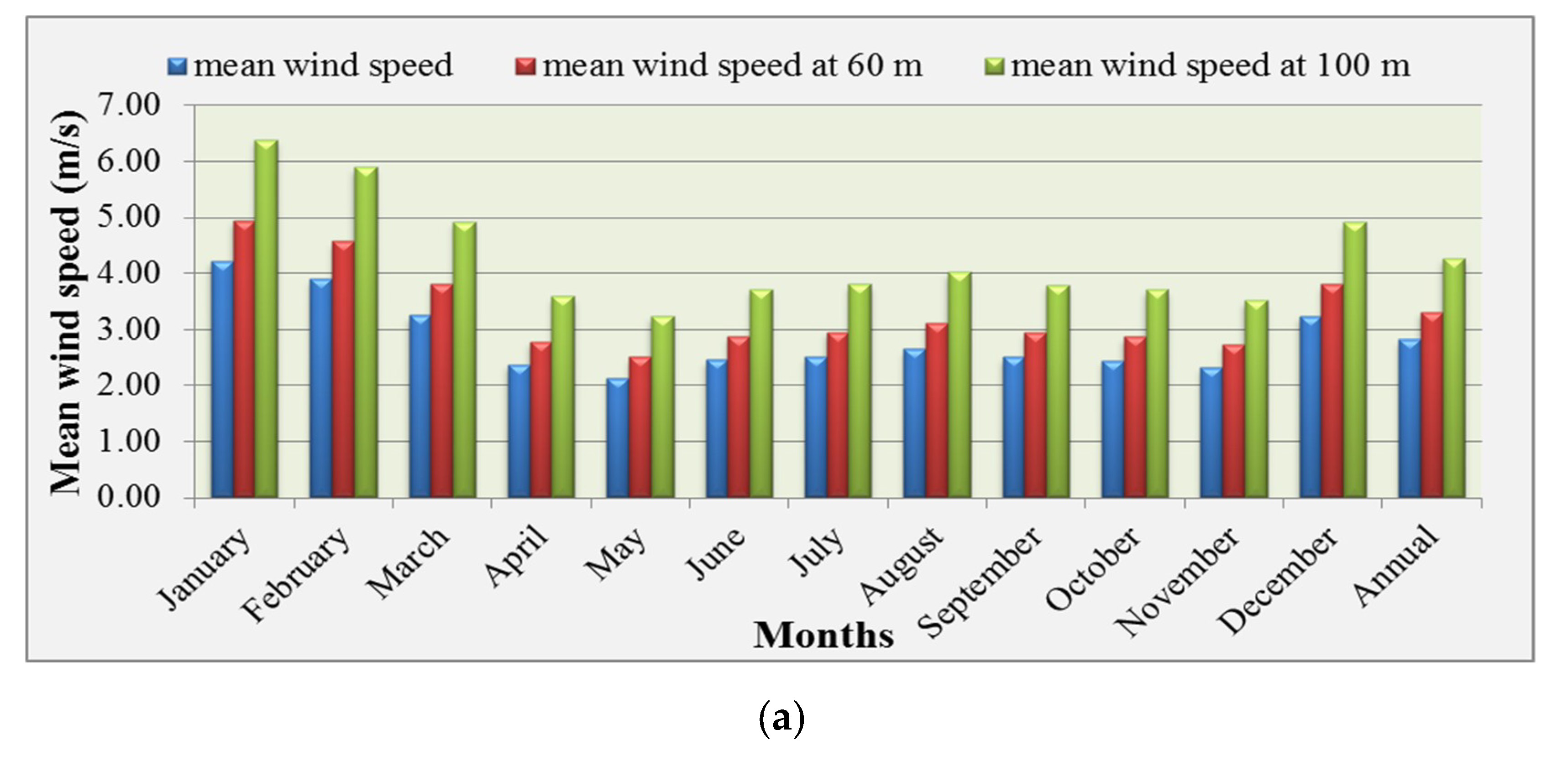
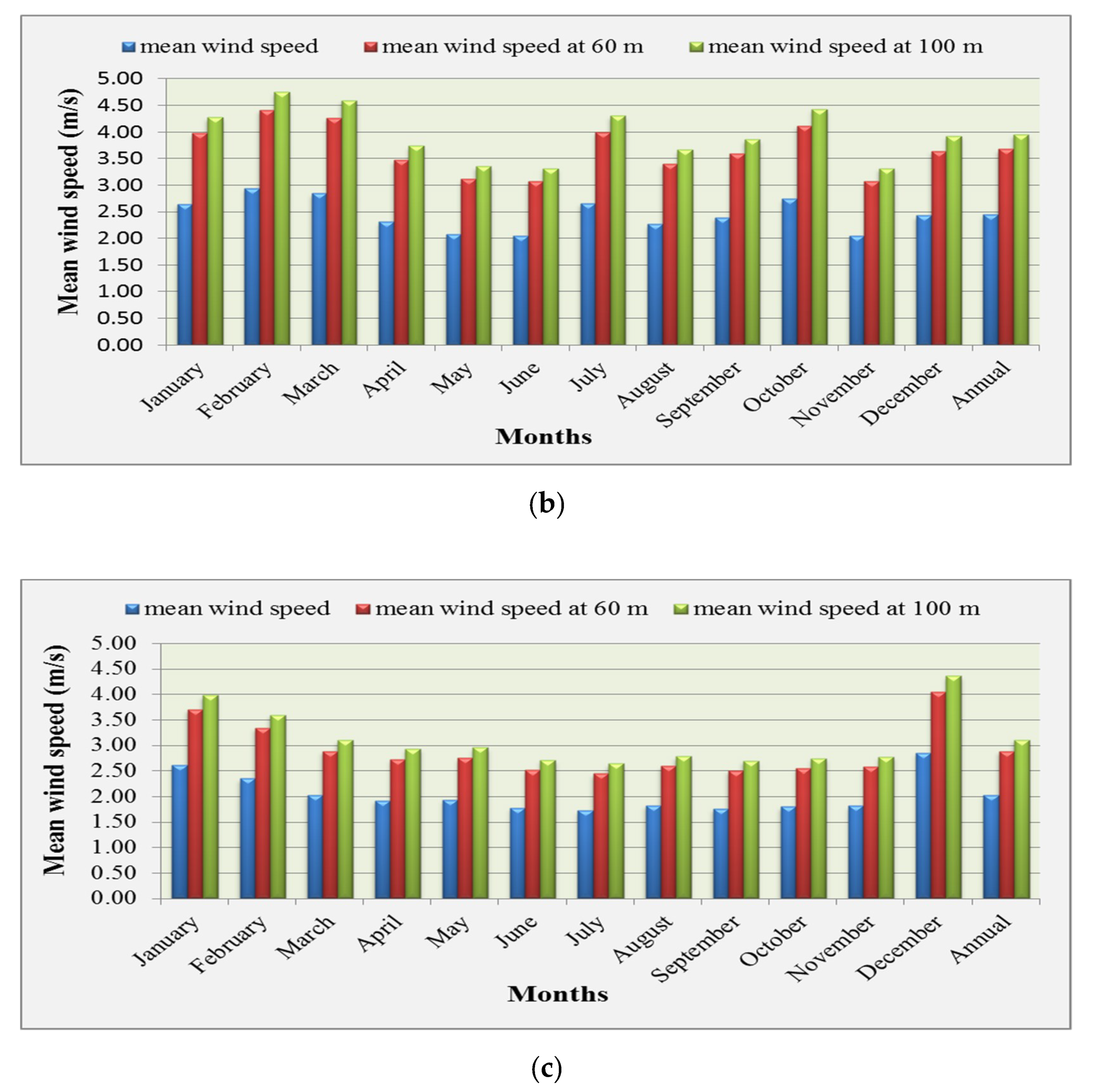
Figure 7.
Comparison of the capacity factors obtained for different wind turbines at various heights for sites (a) Mersing, (b) Kudat, and (c) Kuala Terengganu.
Figure 7.
Comparison of the capacity factors obtained for different wind turbines at various heights for sites (a) Mersing, (b) Kudat, and (c) Kuala Terengganu.

Figure 8.
Simulation of the output power from WTG for the sampling year.

Figure 9.
Simulation of the output power from wind farm for the sampling year.

Figure 10.
The available capacity of the generation system which is superimposed with the chronologically available load model.
Figure 10.
The available capacity of the generation system which is superimposed with the chronologically available load model.
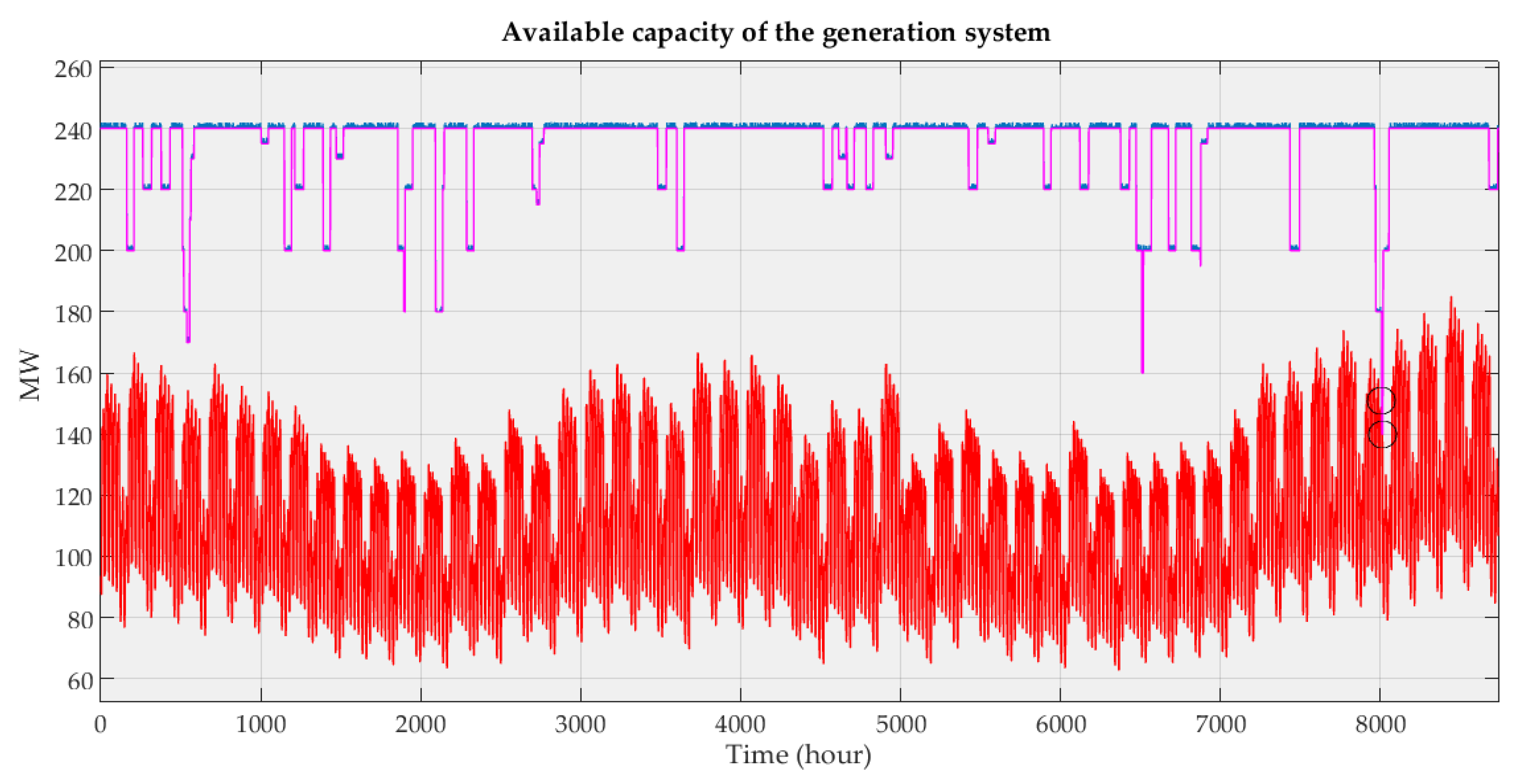
Figure 11.
Simulation of reliability indices with (600) sampling years.

Table 1.
Description of the wind speed stations at selected regions in Malaysia.
| Station | Latitude | Longitude | Altitude (m) |
|---|---|---|---|
| Mersing | 2°27′ N | 103°50′ E | 43.6 |
| Kuala Terengganu | 5°23′ N | 103°06′ E | 5.2 |
| Kudat | 6°55′ N | 116°50′ E | 3.5 |
Table 2.
Monthly and annual mean wind speed (m/s) in Mersing, Kudat, and Kuala Terengganu at different heights above ground level.
Table 2.
Monthly and annual mean wind speed (m/s) in Mersing, Kudat, and Kuala Terengganu at different heights above ground level.
| Wind Observation Station | Months/Year | Annual Mean | |||||||||||
|---|---|---|---|---|---|---|---|---|---|---|---|---|---|
| Jan. | Feb. | Mar. | Apr. | May | Jun. | Jul. | Aug. | Sep. | Oct. | Nov. | Dec. | ||
| Mersing | |||||||||||||
| mean wind speed | 4.22 | 3.89 | 3.24 | 2.36 | 2.13 | 2.45 | 2.51 | 2.65 | 2.50 | 2.44 | 2.32 | 3.24 | 2.82 |
| 60 m | 4.94 | 4.57 | 3.81 | 2.77 | 2.50 | 2.87 | 2.95 | 3.11 | 2.94 | 2.87 | 2.73 | 3.80 | 3.31 |
| 100 m | 6.38 | 5.89 | 4.91 | 3.58 | 3.23 | 3.71 | 3.80 | 4.01 | 3.79 | 3.70 | 3.52 | 4.91 | 4.27 |
| Kudat | |||||||||||||
| mean wind speed | 2.65 | 2.94 | 2.84 | 2.31 | 2.07 | 2.05 | 2.66 | 2.27 | 2.39 | 2.74 | 2.05 | 2.43 | 2.45 |
| 60 m | 3.97 | 4.41 | 4.27 | 3.47 | 3.11 | 3.08 | 4.00 | 3.41 | 3.59 | 4.12 | 3.08 | 3.64 | 3.68 |
| 100 m | 4.28 | 4.75 | 4.59 | 3.73 | 3.35 | 3.31 | 4.30 | 3.66 | 3.86 | 4.43 | 3.31 | 3.92 | 3.95 |
| Kuala Terengganu | |||||||||||||
| mean wind speed | 2.61 | 2.35 | 2.03 | 1.92 | 1.94 | 1.78 | 1.73 | 1.82 | 1.76 | 1.80 | 1.82 | 2.86 | 2.03 |
| 60 m | 3.70 | 3.34 | 2.88 | 2.72 | 2.75 | 2.52 | 2.45 | 2.59 | 2.50 | 2.55 | 2.58 | 4.05 | 2.89 |
| 100 m | 3.98 | 3.59 | 3.10 | 2.93 | 2.96 | 2.71 | 2.64 | 2.78 | 2.69 | 2.75 | 2.77 | 4.36 | 3.10 |
Table 3.
Wind power and energy density characteristics at heights of 43.6 m and 100 m in Mersing.
| A Height of 43.6 m | A Height of 100 m | |||||||||||
|---|---|---|---|---|---|---|---|---|---|---|---|---|
| Months/Year | ⊽ | k | c | PD (w/m2) | Hours | ED (kWh/m2) | ⊽ | k | c | PD (w/m2) | Hours | ED (kWh/m2) |
| January | 4.22 | 5.37 | 4.572 | 52.070 | 747 | 38.896 | 6.38 | 5.37 | 6.922 | 180.702 | 747 | 134.9841 |
| February | 3.89 | 5.68 | 4.209 | 40.532 | 675 | 27.359 | 5.89 | 5.68 | 6.373 | 140.698 | 675 | 94.97137 |
| March | 3.24 | 3.84 | 3.588 | 26.214 | 747 | 19.582 | 4.91 | 3.84 | 5.432 | 90.960 | 747 | 67.94703 |
| April | 2.36 | 3.89 | 2.612 | 10.086 | 723 | 7.292 | 3.58 | 3.89 | 3.955 | 35.014 | 723 | 25.31527 |
| May | 2.13 | 3.26 | 2.381 | 8.010 | 747 | 5.984 | 3.23 | 3.26 | 3.605 | 27.803 | 747 | 20.76847 |
| June | 2.45 | 3.67 | 2.716 | 11.488 | 723 | 8.306 | 3.71 | 3.67 | 4.112 | 39.866 | 723 | 28.823 |
| July | 2.51 | 3.37 | 2.798 | 12.859 | 747 | 9.606 | 3.80 | 3.37 | 4.237 | 44.653 | 747 | 33.35577 |
| August | 2.65 | 3.00 | 2.968 | 16.014 | 747 | 11.962 | 4.01 | 3.00 | 4.494 | 55.591 | 747 | 41.52655 |
| September | 2.50 | 3.35 | 2.788 | 12.746 | 723 | 9.215 | 3.79 | 3.35 | 4.221 | 44.232 | 723 | 31.97939 |
| October | 2.44 | 3.67 | 2.710 | 11.412 | 747 | 8.525 | 3.70 | 3.67 | 4.103 | 39.605 | 747 | 29.58467 |
| November | 2.32 | 3.88 | 2.568 | 9.590 | 723 | 6.934 | 3.52 | 3.88 | 3.887 | 33.257 | 723 | 24.04445 |
| December | 3.24 | 3.45 | 3.604 | 27.287 | 747 | 20.384 | 4.91 | 3.45 | 5.456 | 94.674 | 747 | 70.72135 |
| Annual | 2.82 | 2.25 | 3.221 | 24.370 | - | 17.790 | 4.27 | 2.25 | 4.877 | 84.595 | - | 61.754 |
Table 4.
The technical data of wind turbines.
| Characteristics | P10-20 | 591672E | P12-25 | G-3120 | P15-50 | P25-100 |
|---|---|---|---|---|---|---|
| Rated power (kw) | 20 | 22 | 25 | 35 | 50 | 100 |
| Hub height (m) | - | 30 | - | 42.7 | - | - |
| Rotor diameter (m) | 10 | 15 | 12 | 19.2 | 15.2 | 25 |
| Cut-in wind speed (m/s) | 2.7 | 2 | 2.7 | 3.5 | 2.7 | 2.7 |
| Rated wind speed (m/s) | 10 | 10 | 10 | 8 | 12 | 10 |
| Cut-off wind speed (m/s) | 25 | 25 | 25 | 25 | 25 | 25 |
Table 5.
Reliability indices at various sites in Malaysia.
| Name of Site | Reliability Indices | |||
|---|---|---|---|---|
| LOLE (hrs/year) | LOEE (MWh/year) | LOLF (occ/year) | LOLD (hrs/occ) | |
| Basic RBTS system without wind generation (published) | 1.152 | 11.78 | 0.229 | 4.856 |
| Basic RBTS system without wind generation (computed) | 1.161 | 10.191 | 0.230 | 5.05 |
| Basic RBTS system and (53 × 0.035 = 1.85 MW) wind generators at Mersing site | 1.115 | 9.744 | 0.225 | 4.944 |
| Basic RBTS system and (106 × 0.035 = 3.71 MW) wind generators at Mersing site | 0.987 | 7.357 | 0.220 | 4.486 |
| Basic RBTS system and (53 × 0.035 MW) wind generators at Kudat site | 1.131 | 10.948 | 0.225 | 5.012 |
| Basic RBTS system and (106 × 0.035 = 3.71 MW) wind generators at Kudat site | 1.128 | 10.018 | 0.236 | 4.779 |
Loss of Load Expectation (LOLE)/ LOLE (hour/year); Loss of Energy Expectation (LOEE)/ LOEE (MWh/year); Loss of Load Frequency (LOLF)/ LOLF (occurrence/year); Loss of Load Duration (LOLD)/ LOLD (hour/occurrence).
© 2019 by the authors. Licensee MDPI, Basel, Switzerland. This article is an open access article distributed under the terms and conditions of the Creative Commons Attribution (CC BY) license (http://creativecommons.org/licenses/by/4.0/).
Share and Cite
MDPI and ACS Style
Ali Kadhem, A.; Abdul Wahab, N.I.; N. Abdalla, A. Wind Energy Generation Assessment at Specific Sites in a Peninsula in Malaysia Based on Reliability Indices. Processes 2019, 7, 399. https://doi.org/10.3390/pr7070399
AMA Style
Ali Kadhem A, Abdul Wahab NI, N. Abdalla A. Wind Energy Generation Assessment at Specific Sites in a Peninsula in Malaysia Based on Reliability Indices. Processes. 2019; 7(7):399. https://doi.org/10.3390/pr7070399
Chicago/Turabian StyleAli Kadhem, Athraa, Noor Izzri Abdul Wahab, and Ahmed N. Abdalla. 2019. "Wind Energy Generation Assessment at Specific Sites in a Peninsula in Malaysia Based on Reliability Indices" Processes 7, no. 7: 399. https://doi.org/10.3390/pr7070399
Note that from the first issue of 2016, this journal uses article numbers instead of page numbers. See further details here.