Mold Level Predict of Continuous Casting Using Hybrid EMD-SVR-GA Algorithm


Abstract
:1. Introduction
2. Basic Algorithm Research
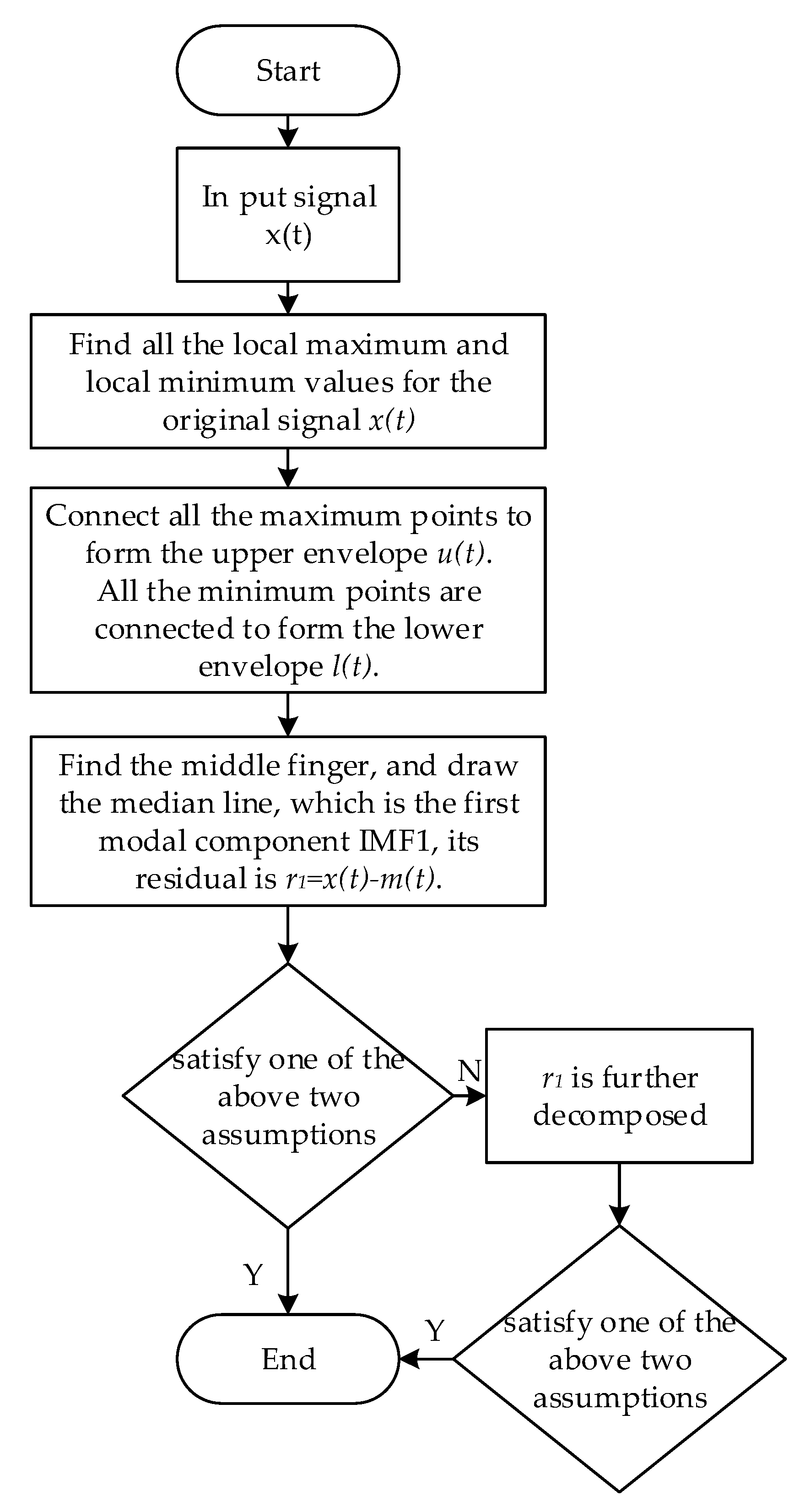
2.1. EMD Algorithm
- (1)
- In the entire data set, the number of extreme values and the number of zero crossings must be equal or at most have one point of difference.
- (2)
- At any point, the average is defined by the local maximum envelope, and the minimum envelope is zero.
2.2. SVR Algorithm
3. Hybrid Algorithm Research
3.1. Feasibility Analyses
3.2. The Full Procedure of EMD-SVRGA
4. Experiments Studies
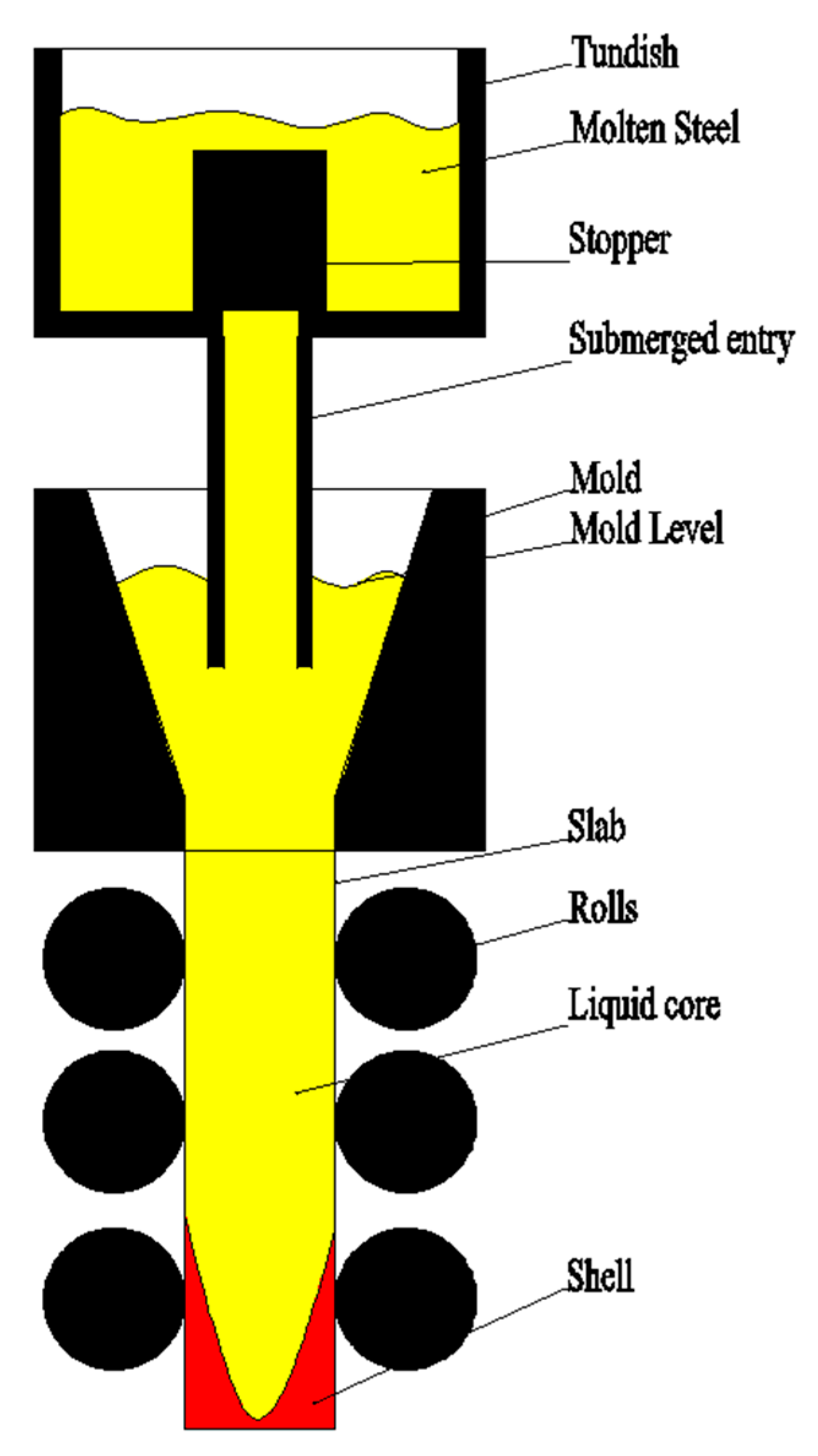
4.1. Problem Prescription
4.2. EMD-SVR
4.3. Experimental Results and Analyses
4.4. Predicting Accuracy Significance Tests
5. Conclusions
Author Contributions
Funding
Acknowledgments
Conflicts of Interest
Nomenclature
| EMD | Empirical mode decomposition |
| IMF | Intrinsic mode function |
| TS | Time series |
| ARMA | Autoregressive moving average |
| ACF | Autocorrelation function |
| PACF | Partial autocorrelation function |
| SVR | Support vector regression |
| GA | Genetic Algorithm |
| WT | Wavelet Transform |
| CC | Correlation Coefficient |
| RMSE | Root-mean-square error |
| MAE | Mean Absolute Error |
References
- Ataka, M. Rolling Technology and Theory for the Last 100 Years: The Contribution of Theory to Innovation in Strip Rolling Technology. ISIJ Int. 2015, 55, 89–102. [Google Scholar] [CrossRef] [Green Version]
- Jin, X.; Chen, D.F.; Zhang, D.J.; Xie, X.; Bi, Y.Y. Water model study on fluid flow in slab continuous casting mould with solidified shell. Ironmak. Steelmak. 2011, 38, 155–159. [Google Scholar] [CrossRef]
- Shen, B.Z.; Shen, H.F.; Liu, B.C. Water modelling of level fluctuation in thin slab continuous casting mould. Ironmak. Steelmak. 2009, 36, 33–38. [Google Scholar] [CrossRef]
- Wang, X.; Zhang, S.; Yao, M.; Ma, H.; Zhang, X. Effect of casting process on mould friction during wide, thick slab continuous casting. Ironmak. Steelmak. 2014, 41, 464–473. [Google Scholar] [CrossRef]
- Lynch, P. The origins of computer weather prediction and climate modeling. J. Comput. Phys. 2008, 227, 3431–3444. [Google Scholar] [CrossRef]
- Weron, R. Electricity price predicting: A review of the state-of-the-art with a look into the future. Int. J. Predict. 2014, 30, 1030–1081. [Google Scholar] [CrossRef]
- Lee, W.-J.; Hong, J. A hybrid dynamic and fuzzy time series model for mid-term power load predicting. Int. J. Electr. Power Energy Syst. 2015, 64, 1057–1062. [Google Scholar] [CrossRef]
- Dai, S.; Niu, D.; Li, Y. Daily Peak Load Predicting Based on Complete Ensemble Empirical Mode Decomposition with Adaptive Noise and Support Vector Machine Optimized by Modified Grey Wolf Optimization Algorithm. Energies 2018, 11, 163. [Google Scholar] [CrossRef]
- Wang, W.-C.; Chau, K.-W.; Cheng, C.-T.; Qiu, L. A comparison of performance of several artificial intelligence methods for predicting monthly discharge time series. J. Hydrol. 2009, 374, 294–306. [Google Scholar] [CrossRef]
- Azad, H.B.; Mekhilef, S.; Ganapathy, V.G. Long-Term Wind Speed Predicting and General Pattern Recognition Using Neural Networks. IEEE Trans. Sustain. Energy 2014, 5, 546–553. [Google Scholar] [CrossRef]
- Gaudioso, M.; Gorgone, E.; Labbe, M.; Rodriguez-Chia, A.M. Lagrangian relaxation for SVM feature selection. Comput. Oper. Res. 2017, 87, 137–145. [Google Scholar] [CrossRef] [Green Version]
- Wang, J.; Shi, P.; Jiang, P.; Hu, J.; Qu, S.; Chen, X.; Chen, Y.; Dai, Y.; Xiao, Z. Application of BP Neural Network Algorithm in Traditional Hydrological Model for Flood Predicting. Water 2017, 9, 48. [Google Scholar] [CrossRef]
- He, F.; Zhang, L. Mold breakout prediction in slab continuous casting based on combined method of GA-BP neural network and logic rules. Int. J. Adv. Manuf. Technol. 2018, 95, 4081–4089. [Google Scholar] [CrossRef]
- Fan, G.-F.; Peng, L.-L.; Hong, W.-C.; Sun, F. Electric load predicting by the SVR model with differential empirical mode decomposition and auto regression. Neurocomputing 2016, 173, 958–970. [Google Scholar] [CrossRef]
- Nie, H.; Liu, G.; Liu, X.; Wang, Y. Hybrid of ARIMA and SVMs for Short-Term Load Predicting. Energy Procedia 2012, 16, 1455–1460. [Google Scholar] [CrossRef]
- Liu, Y.; Gao, Z. Enhanced just-in-time modelling for online quality prediction in BF ironmaking. Ironmak. Steelmak. 2015, 42, 321–330. [Google Scholar] [CrossRef]
- Cincotti, S.; Gallo, G.; Ponta, L.; Raberto, M. Modeling and predicting of electricity spot-prices: Computational intelligence vs classical econometrics. Ai Commun. 2014, 27, 301–314. [Google Scholar] [CrossRef]
- Ghosh, S.K.; Ganguly, S.; Chattopadhyay, P.P.; Datta, S. Effect of copper and microalloying (Ti, B) addition on tensile properties of HSLA steels predicted by ANN technique. Ironmak. Steelmak. 2009, 36, 125–132. [Google Scholar] [CrossRef]
- Hong, W.-C. Chaotic particle swarm optimization algorithm in a support vector regression electric load predicting model. Energy Convers. Manag. 2009, 50, 105–117. [Google Scholar] [CrossRef]
- Voyant, C.; Muselli, M.; Paoli, C.; Nivet, M.-L. Numerical weather prediction (NWP) and hybrid ARMA/ANN model to predict global radiation. Energy 2012, 39, 341–355. [Google Scholar] [CrossRef] [Green Version]
- Ren, Y.; Suganthan, P.N.; Srikanth, N. A Comparative Study of Empirical Mode Decomposition-Based Short-Term Wind Speed Predicting Methods. IEEE Trans. Sustain. Energy 2015, 6, 236–244. [Google Scholar] [CrossRef]
- Ye, L.; Liu, P. Combined Model Based on EMD-SVM for Short-term Wind Power Prediction. Proc. CSEE 2011, 31, 102–108. [Google Scholar]
- Lei, Y.G.; Lin, J.; He, Z.J.; Zuo, M.J. A review on empirical mode decomposition in fault diagnosis of rotating machinery. Mech. Syst. Signal Process. 2013, 35, 108–126. [Google Scholar] [CrossRef]
- Huang, N.E.; Shen, Z.; Long, S.R.; Wu, M.L.C.; Shih, H.H.; Zheng, Q.N.; Yen, N.C.; Tung, C.C.; Liu, H.H. The empirical mode decomposition and the Hilbert spectrum for nonlinear and non-stationary time series analysis. Proc. R. Soc. A Math. Phys. Eng. Sci. 1998, 454, 903–995. [Google Scholar] [CrossRef]
- Bajaj, V.; Pachori, R.B. Classification of Seizure and Nonseizure EEG Signals Using Empirical Mode Decomposition. IEEE Trans. Inf. Technol. Biomed. 2012, 16, 1135–1142. [Google Scholar] [CrossRef] [PubMed]
- Priya, A.; Yadav, P.; Jain, S.; Bajaj, V. Efficient method for classification of alcoholic and normal EEG signals using EMD. J. Eng. 2018, 2018, 166–172. [Google Scholar] [CrossRef]
- Prasanna Kumar, M.K.; Kumaraswamy, R. Single-channel speech separation using combined EMD and speech-specific information. Int. J. Speech Technol. 2017, 20, 1037–1047. [Google Scholar] [CrossRef]
- Guo, Z.; Zhao, W.; Lu, H.; Wang, J. Multi-step predicting for wind speed using a modified EMD-based artificial neural network model. Renew. Energy 2012, 37, 241–249. [Google Scholar] [CrossRef]
- Tang, J.; Zhao, L.; Yue, H.; Yu, W.; Chai, T. Vibration Analysis Based on Empirical Mode Decomposition and Partial Least Square. Procedia Energy 2011, 16, 646–652. [Google Scholar] [CrossRef] [Green Version]
- Xu, G.; Tian, W.; Qian, L. EMD- and SVM-based temperature drift modeling and compensation for a dynamically tuned gyroscope (DTG). Mech. Syst. Signal Process. 2007, 21, 3182–3188. [Google Scholar] [CrossRef]
- Luo, L.; Yan, Y.; Xie, P.; Sun, J.; Xu, Y.; Yuan, J. Hilbert-Huang transform, Hurst and chaotic analysis based flow regime identification methods for an airlift reactor. Chem. Eng. J. 2012, 181, 570–580. [Google Scholar] [CrossRef]
- Srinivasan, R.; Rengaswamy, R.; Miller, R. A modified empirical mode decomposition (EMD) process for oscillation characterization in control loops. Control Eng. Pract. 2007, 15, 1135–1148. [Google Scholar] [CrossRef]
- Zhang, X.Y.; Zhou, J.Z. Multi-fault diagnosis for rolling element bearings based on ensemble empirical mode decomposition and optimized support vector machines. Mech. Syst. Signal Process. 2013, 41, 127–140. [Google Scholar] [CrossRef]
- Dong, Y.; Zhang, Z.; Hong, W.-C. A Hybrid Seasonal Mechanism with a Chaotic Cuckoo Search Algorithm with a Support Vector Regression Model for Electric Load Predicting. Energies 2018, 11, 1009. [Google Scholar] [CrossRef]
- Fan, G.-F.; Peng, L.-L.; Hong, W.-C. Short term load predicting based on phase space reconstruction algorithm and bi-square kernel regression model. Appl. Energy 2018, 224, 13–33. [Google Scholar] [CrossRef]
- Wilcoxon, F. Individual comparisons by ranking methods. Biom. Bull. 1945, 1, 80–83. [Google Scholar] [CrossRef]
- Friedman, M. A comparison of alternative tests of significance for the problem of m rankings. Ann. Math. Stat. 1940, 11, 86–92. [Google Scholar] [CrossRef]


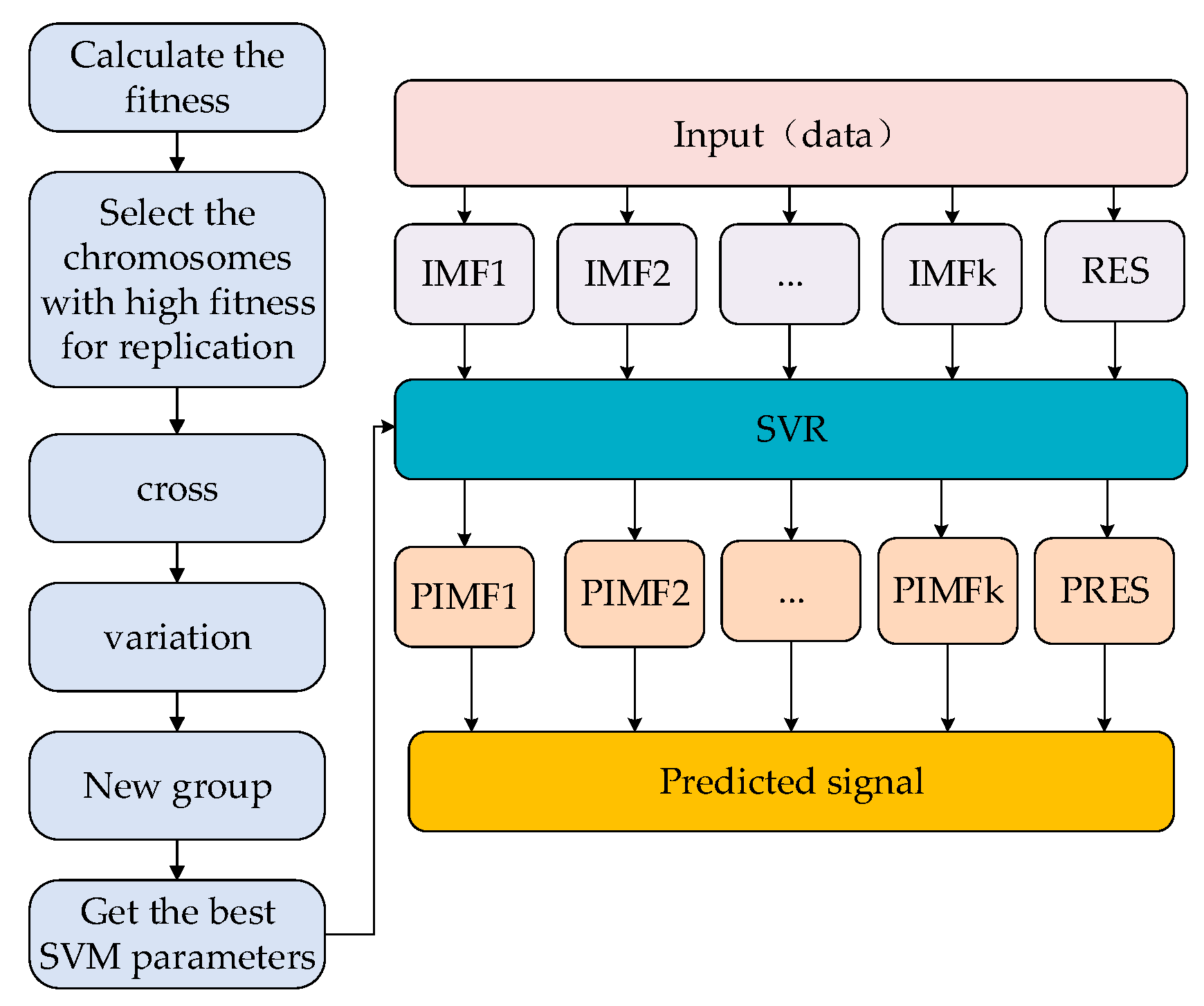
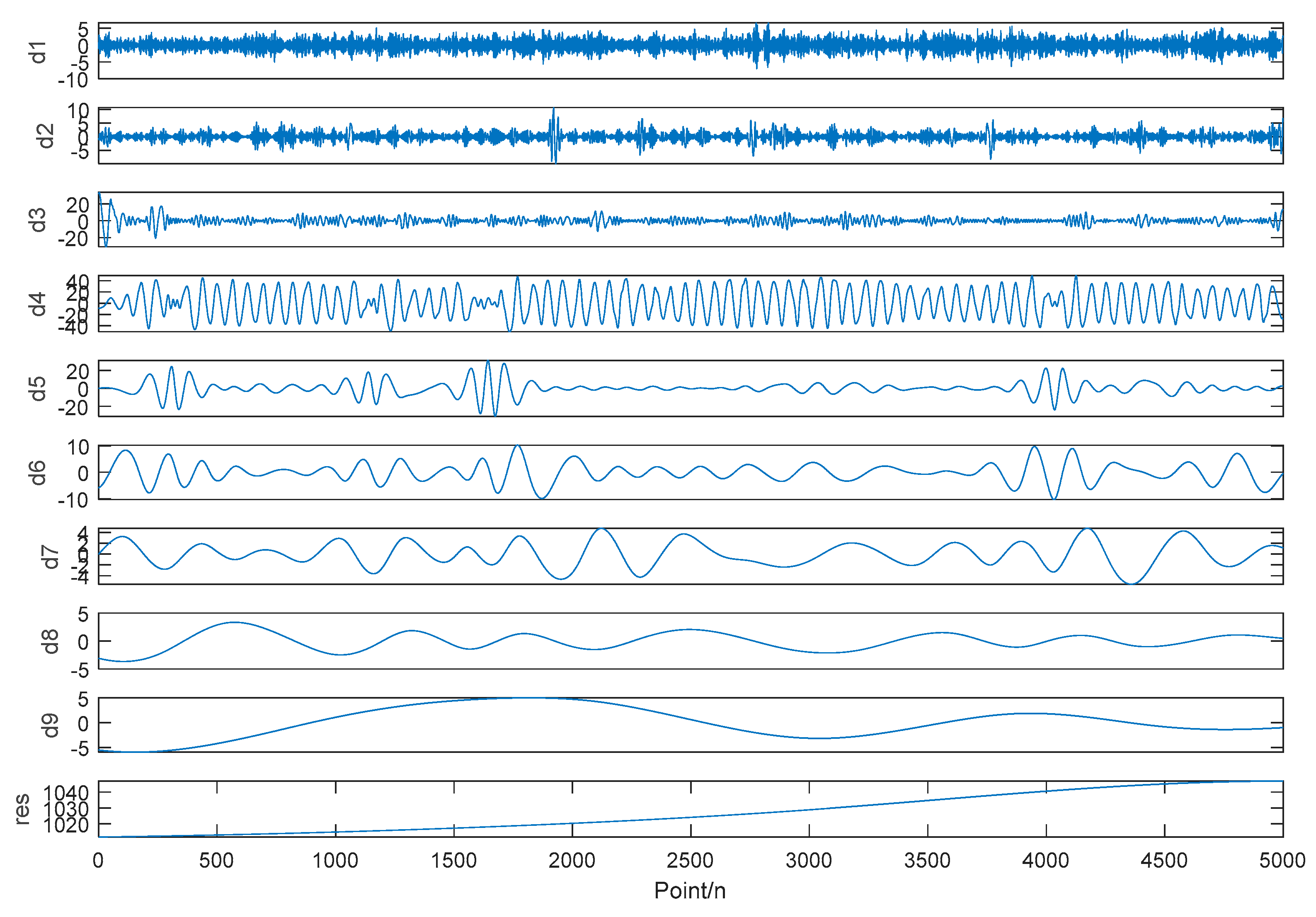
| Step 1. Decompose the mold level signal data into several IMFs and one residual by the EMD. Step 2. Global optimization of C and g in SVR is performed using GA to determine the SVR model. Step 3. Predicted IMFs (PIMF) obtained by SVR for each IMF. Step 4. Predicted residual sequence obtained by SVR for residual sequence. Step 5. Sum all predicted IMFs and residual sequences to obtain the predicted signal. |
| Project | Specification |
|---|---|
| Continuous casting machine model | Curved continuous caster |
| Secondary cooling category | Aerosol cooling, dynamic water distribution |
| Gap control | Remote adjustment, dynamic soft reduction |
| Basic arc radius/mm | 9500 |
| Mold length/mm | 900 |
| Metallurgical length/mm | 39,200 |
| Mold vibration frequency/time/min | 25–400 |
| Mold vibration amplitude/mm | 2–10 |
| Slab width/mm | 900–2150 |
| Slab thickness/mm | 230/250 |
| Working speed/m/min | 0.8–2.03 |
| Project | Mold Level |
|---|---|
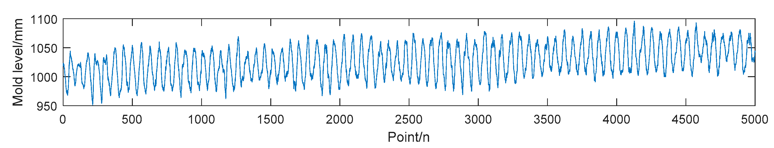
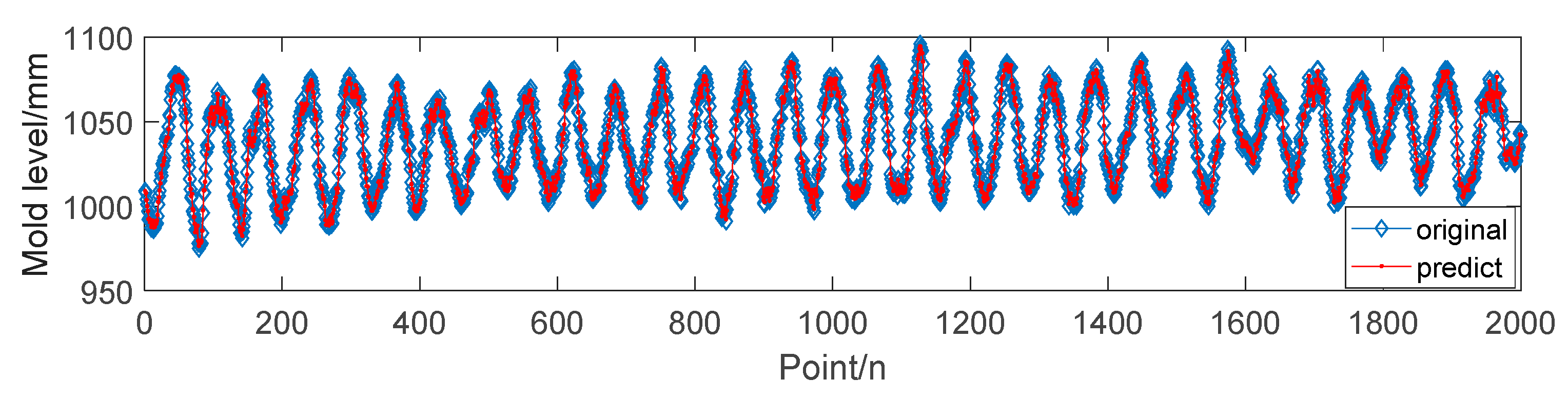
| Max-Min Values (mm) | 951–1096 |
| Mean (mm) | 1026.7607 |
| Standard Deviation (mm) | 28.3495 |
| Skewness | −0.02506 |
| Kurtosis | 2.1049 |
| C | g | ACF | PACF | |
|---|---|---|---|---|
| WT-ARMA | - | - | 2 | 2 |
| WT-SVR | 100 | 1 | - | - |
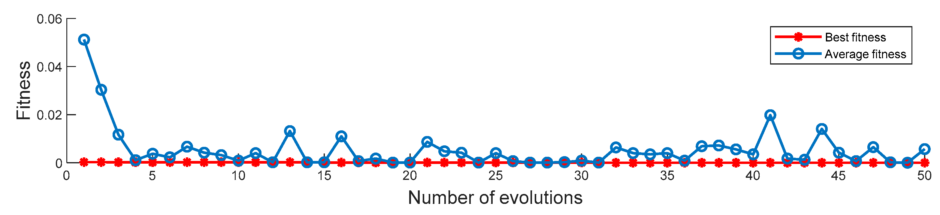
| WT-SVRGA | 16.3485 | 0.01773 | - | - |
| EMD-ARMA | - | - | 2 | 2 |
| EMD-SVR | 100 | 1 | - | - |
| EMD-SVRGA | 95.5729 | 0.39511 | - | - |
| R | RMSE | MAE | |
|---|---|---|---|
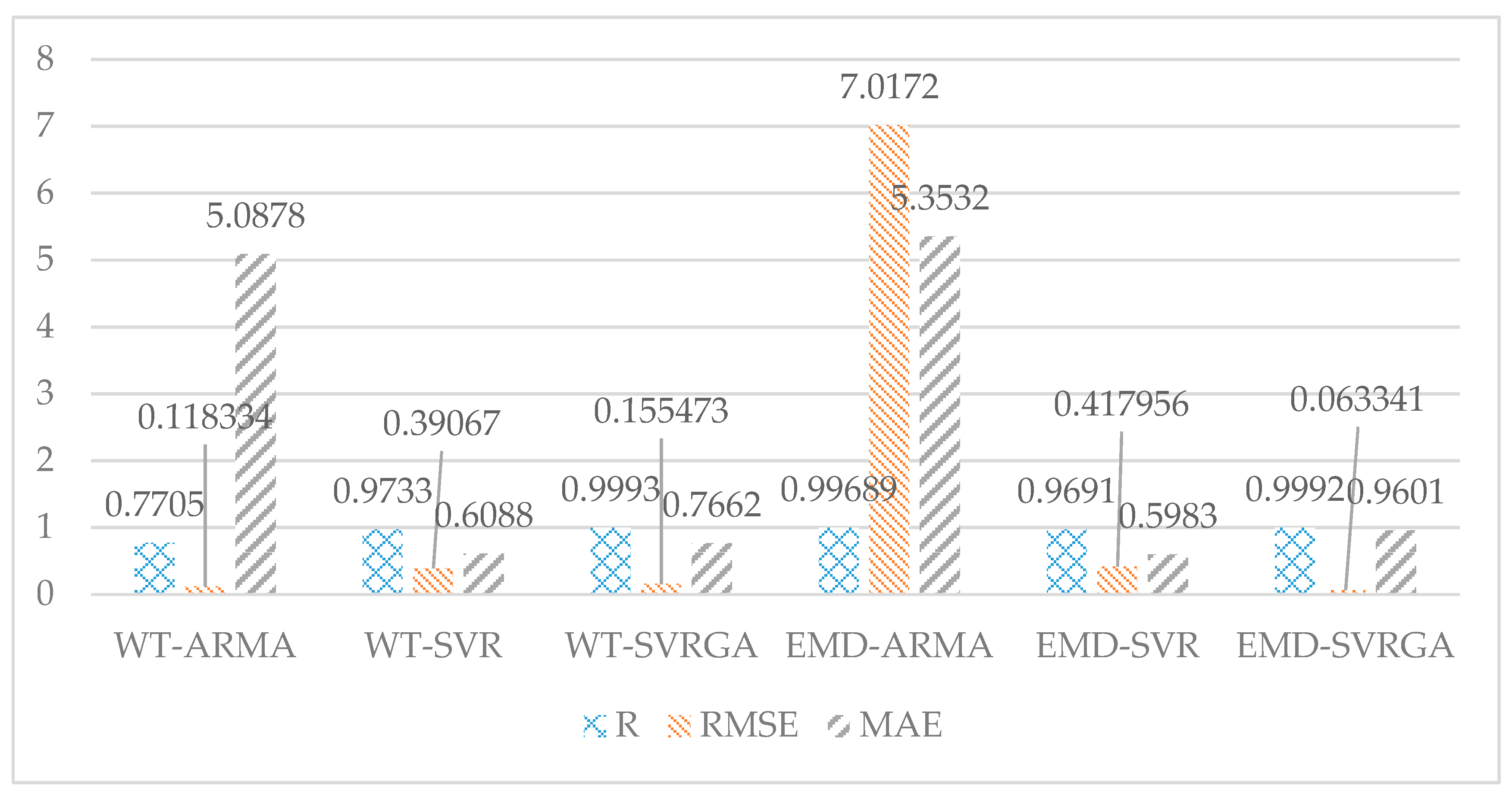
| WT-ARMA | 0.7705 | 0.118334 | 5.0878 |
| WT-SVR | 0.9733 | 0.390670 | 0.6088 |
| WT-SVRGA | 0.9993 | 0.155473 | 0.7662 |
| EMD-ARMA | 0.99689 | 7.0172 | 5.3532 |
| EMD-SVR | 0.9691 | 0.417956 | 0.5983 |
| EMD-SVRGA | 0.9992 | 0.063341 | 0.9601 |
| Compared Models | Wilcoxon Signed-Rank Test | Friedman Test | |||
|---|---|---|---|---|---|
| α = 0.025 | α = 0.05 | α = 0.05 | |||
| h-Value | p-Value | h-Value | p-Value | ||
| EMD-SVRGA vs. WT-ARMA | 1 | 0 | 1 | 0 | H0: The results of the six algorithms are equal F = 35.8 p = 0 (Reject H0) |
| EMD-SVRGA vs. WT-SVR | 1 | 0 | 1 | 0 | |
| EMD-SVRGA vs. WT-SVRGA | 1 | 0 | 1 | 0 | |
| EMD-SVRGA vs. EMD-ARMA | 1 | 0 | 1 | 0 | |
| EMD-SVRGA vs. EMD-SVR | 1 | 0 | 1 | 0 | |
© 2019 by the authors. Licensee MDPI, Basel, Switzerland. This article is an open access article distributed under the terms and conditions of the Creative Commons Attribution (CC BY) license (http://creativecommons.org/licenses/by/4.0/).
Share and Cite
Lei, Z.; Su, W. Mold Level Predict of Continuous Casting Using Hybrid EMD-SVR-GA Algorithm. Processes 2019, 7, 177. https://doi.org/10.3390/pr7030177
Lei Z, Su W. Mold Level Predict of Continuous Casting Using Hybrid EMD-SVR-GA Algorithm. Processes. 2019; 7(3):177. https://doi.org/10.3390/pr7030177
Chicago/Turabian StyleLei, Zhufeng, and Wenbin Su. 2019. "Mold Level Predict of Continuous Casting Using Hybrid EMD-SVR-GA Algorithm" Processes 7, no. 3: 177. https://doi.org/10.3390/pr7030177
APA StyleLei, Z., & Su, W. (2019). Mold Level Predict of Continuous Casting Using Hybrid EMD-SVR-GA Algorithm. Processes, 7(3), 177. https://doi.org/10.3390/pr7030177