Article

A Systematic Grey-Box Modeling Methodology via Data Reconciliation and SOS Constrained Regression

1
Systems Engineering and Automatic Control department, EII, Universidad de Valladolid, C/Real de Burgos s/n, 47011 Valladolid, Spain
2
Instituto Universitario de Automática e Informática Industrial (ai2), Universitat Politècnica de Valencia, Camino de Vera S/N, 46022 Valencia, Spain
3
Institute of Sustainable Processes (IPS), Universidad de Valladolid, C/Real de Burgos s/n, 47011 Valladolid, Spain
*
Author to whom correspondence should be addressed.
Processes 2019, 7(3), 170; https://doi.org/10.3390/pr7030170
Submission received: 26 February 2019 / Revised: 15 March 2019 / Accepted: 20 March 2019 / Published: 23 March 2019
(This article belongs to the Special Issue Process Modelling and Simulation)

Abstract

:
Developing the so-called grey box or hybrid models of limited complexity for process systems is the cornerstone in advanced control and real-time optimization routines. These models must be based on fundamental principles and customized with sub-models obtained from process experimental data. This allows the engineer to transfer the available process knowledge into a model. However, there is still a lack of a flexible but systematic methodology for grey-box modeling which ensures certain coherence of the experimental sub-models with the process physics. This paper proposes such a methodology based in data reconciliation (DR) and polynomial constrained regression. A nonlinear optimization of limited complexity is to be solved in the DR stage, whereas the proposed constrained regression is based in sum-of-squares (SOS) convex programming. It is shown how several desirable features on the polynomial regressors can be naturally enforced in this optimization framework. The goodnesses of the proposed methodology are illustrated through: (1) an academic example and (2) an industrial evaporation plant with real experimental data.

1. Introduction

Due to the increasing levels of digitalization, motivated by the ideas of the so-called Industry 4.0 [1], both academic researchers and technological companies search for methods to transform raw data in useful information. This information is expected to significantly impact in the decision-making procedures at all levels in a factory: from operation and maintenance to production scheduling and supply chain.
The process industries are not alien to this digital transformation, although the challenges to face are slightly different from the ones in other sectors. On the one hand, their activity is based in complex plants formed by very heterogeneous (usually expensive) equipment, performing complex processes such as (bio)chemical reactions, phase transformations, etc. On the other hand, their markets are quite constrained in terms of raw materials or product demands, whereas environmental regulations become tighter every year. In this context, improved efficiency thanks to smart-production systems can be achieved by: (1) transforming data in reliable information and use such information to optimize the operation [2] and (2) improve the coordination of tasks in a plant [3] and between plants [4]—in summary, to equip people (operators, engineers, managers, etc.) with support systems in order to make better tactical decisions.
Suitable models of a different nature are key to making better decisions through the above stages. Current trends encourage the use of pure data-driven approaches coming from the framework of artificial intelligence and big data (e.g., artificial neural networks [5] and machine learning [6]). These techniques are rather systematic and do not require a deep knowledge on the systems where applied. Nevertheless, the process industry is not characterized by a scarce knowledge on the involved physicochemical processes. Indeed, detailed models for some equipment/plants have already existed for the last two decades (e.g., distillation columns [7]). Therefore, throwing out all this deep knowledge and just relying on the decisions inferred by data-driven machines would be risky.
These high-fidelity models have normally been used in offline simulations, for making decisions about the process design. This drawback is due to the usually high computational complexity and the relatively limited degrees of freedom to fit the actual plants. Therefore, there is still a lack of suitable models able for online prediction at almost all tactical levels of the automation pyramid: from real-time predictive simulation and optimization [8] to production planning and scheduling [3]. Therefore, the concept of plant digital twin contains a (virtual replica of actual assets that matches their behavior in real time), playing an important role in decision-support systems.
Consequently, many people in the process control community have been devoting efforts during the last decade to develop efficient and reliable models to support operators and managers in their decisions [9,10]. The preferred option is building models that combine as much physical information as possible/acceptable with relationships obtained from experimental data collected from the plant [11]. In this way, these hybrid or grey-box models get a high level of matching with the actual plant and, importantly, they get improved prediction capabilities as their outputs will at least fulfil the basic physical laws considered.
There are many good reviews and publications on process modelling, both covering first principles [12] and data-based approaches [13], but, in the authors’ opinion, there is still a lack of methodology for the systematic development of grey-box models. In addition, several different approaches have been proposed in the literature to identify the “black part” of the grey-box model from input–output data. Among them, least-squares (LS) regression with regularization in the model coefficients [14,15] is one of the most used. Nonetheless, although the obtained models with this family of methods are quite balanced in terms of fitness to data and model complexity, the guarantees of physical coherence are under discussion, as they mainly depend on the quality and quantity of the collected data for regression.
This paper proposes a two-stage methodology which combines robust data reconciliation [16] with improved constrained regression. In the first stage, one gets estimations for all process variables that are coherent with some basic physical laws. Then, in a second stage of experimental customization, sophisticated constrained regression is used to get reliable experimental relationships among variables (that are not necessarily physical inputs and outputs measured in the plant), which will complete the first-principles backbone [17].
In this context, the authors of [18,19] already proposed a useful concept for black-box modeling: a machine-learning approach which automatically selects the suitable model complexity among a set of basis functions by balancing some model-complexity criteria with the fitness to regression data. Thus, this approach can be used in the second stage (constrained regression) of our proposed grey-box model building methodology [17]. The goal in this stage is to include as much process knowledge as possible (bounds on the model response, valid input domain, monotonic responses, maximum slopes and curvatures, etc.) as constraints in the regression. However, as these types of constraints on the model need to be enforced on infinitely many points belonging to the input–output domain, the regression becomes a semi-infinite programming problem [20] where a set of finite decision variables (the model parameters) but an infinite set of constraints arise. To tackle this problem numerically, the authors of [18] break down the problem into two parts: first, a relaxation of the original problem over a finite subset x X of the inputs domain X X (typically the points in the regression dataset) is solved via mixed-integer programming (MIP). Once a solution (i.e., values of the n model coefficients β R n ) for this problem is gathered, a subsequent maximum-violation problem needs to be solved—that is, basically, a maximization of the constraints violation over all x X , with the model fixed from the previous stage. If the constraints are violated at some point, this is added to the regression dataset and the procedure repeats until no constraint violation is detected. In the general case, this procedure involves solving nonlinear optimization problems (except the MIP one if candidate basis functions and constraints are chosen to be linear in decision variables). Moreover, the problem of finding the point where maximum constraint violation takes place is generally nonconvex. Therefore, a global optimizer is required to guarantee that the best fit fulfilling constraints have been found. Altogether, this means that the constrained-regression problem can be very time-consuming and computationally demanding.
To overcome this issue, in this paper, we propose casting the constrained-regression problem as a sum-of-squares (SOS) polynomial programming one, a technique that emerged ten years ago as the generalization of the semidefinite programming to the polynomial optimization over semi-algebraic sets [21]. The great advantage of SOS programming is the ability of guaranteeing constraint satisfaction for all x X (infinitely-constrained problem) without the need for fine-sampling datasets and via convex optimization. Although SOS programming is quite popular now within the automatic-control community, it has not penetrated too much into other fields of application. In particular, the authors only know one work on SOS programming applied to constrained regression [22], where explicit equilibrium approximations of fast-reacting species are sought via polynomial regressors. This work is particularly interesting because its authors outlined ideas similar to ours about grey-box modeling: they searched for reduced-order representations of kinetic networks which were physically consistent. In this paper, such an initial approach is extended to pose a constrained regression problem with guaranteed satisfaction of more advanced constraints than just model positivity, e.g., boundary constraints and limits on the model (partial) derivatives.
The rest of the article is organized as follows: Section 2 presents the problem formulation and its context in a formal way. The necessary definitions and preliminary results supporting the methodology and/or the examples are summarized in Section 3. Subsequently, Section 4 presents our proposed grey-box modeling methodology and Section 5 goes deeper into the SOS constrained regression. The benefits of the proposal are illustrated in Section 6 with two examples, one academic and another based on an industrial case study. Finally, the results are discussed in the last section, providing final remarks as well as an overview for possible extensions of the method.

2. Problem Statement

Let us assume that some first-principles equations of a process are available:
d x d t = f ( x ( t ) , u ( t ) , z ( t ) , θ ) , h ( x ( t ) , u ( t ) , z ( t ) , θ ) = 0 ,
where x R n is the state vector, u R m are known process inputs (manipulated variables or measured disturbances taking arbitrary values independently of the rest of the variables), z R q are algebraic variables (with not-yet-fixed roles: some of them may be arbitrary inputs, some others may be functions of other variables, as discussed below), θ R ρ are model parameters (assumed to be constant) and f ( · ) R n , h ( · ) R l can be nonlinear functions of their arguments.
Let us also assume that the above model is “incomplete”, meaning that the system (1) is not fully determined by only the inputs u. Formally, this means that there are q n l m > 0 variables z z assumed arbitrarily time-varying. However, some of them are not unknown inputs actually, but must be a function of other variables z ( x , u , z ) , representing the not well-known parts of the process. Therefore, assuming no significant unmodeled dynamics, let us assert that some additional equations r ( x , u , z ) = 0 need to be identified from process experimental data. Note that, although the first-principle model was “complete”, it incorporates parameters θ whose value is not perfectly known. Therefore, stages of data collection and parameter identification are always present in practice, so that the model outputs fit those of the plant.
The classical way to approach this problem is to set up a certain functional structure for the equations r ( x , u , z , θ z ) = 0 searched with some parameters θ z left for identification, and then formulate the following least-squares (LS) constrained (nonlinear) regression problem with N data samples collected at time instants t 1 , t 2 , , t N [23]:
min θ , x 0 t = t 1 t N y ^ ( t ) y ( t ) / σ 2 2 , s . t . : d x d t = f ( x ( t ) , u ( t ) , z ( t ) , θ ) , x ( 0 ) = x 0 , h ( x ( t ) , u ( t ) , z ( t ) , θ ) = 0 , r ( x ( t ) , u ( t ) , z ( t ) , θ z ) = 0 ,
where y ^ are the process measured outputs, normalized by their respective mean or standard deviation σ , and y = c ( x , z ) are their corresponding model predictions.
Note that, in many cases, x 0 may itself be part of the adjustable parameters (initial condition fitting).
This approach assumes that the chosen structure (implicitly in whichever equations are asserted in the expression of r ( · ) = 0 ) for z ( x , u , z ) is correct and the parameters are being estimated in the right way. Therefore, a proper selection of this structure is key to obtaining a good fitness with the real plant. However, the above assumptions and expectations may fail due to the following reasons:
  • Proposing a good candidate structure often implies certain knowledge of the interactions and phenomena taking place in the process, which are normally too complex to model or are not well understood.
  • Some parameters θ z may not be identifiable within reasonable precision with a scarce set of measured variables y.
Furthermore, as problem (2) is normally a nonlinear dynamic optimization one, the computational demands can exploit rapidly with the size of the dataset N, with the complexity of the model equations and the time scales of the involved dynamics [24]. Therefore, it is not recommended to unnecessarily go deep into the physical phenomena as long as the final aim does not require it, e.g., different model requirements arise for the development of digital twins than for the ones for control or optimization purposes.
Hence, as the initially proposed structure r ( · ) will likely not be correct in a complex identification setup, the fit will need to be repeated with a modified candidate structure, following a very time-consuming trial-and-error procedure, without any guarantee of optimality of course.
In these cases, it may be sensible to combine what is known with certainty about the model, such as mass or energy balances, with data-driven equations obtained from measurements, representing those parts of the process which are unknown or complex to model. This results in a grey box model being a mixture of first-principles and data-driven equations [25].

Pursued Goal

As these grey-box models are built to be used for interpolation and extrapolation in control and optimization routines, the data-driven parts must be in coherence with the process physics [26]. Hence, some properties on z and/or in their derivatives (bounds, monotony, curvature, convexity, etc.) would like to be ensured, not only in the regression data but in the entire expected region of operation.
Machine learning is thus recalled to identify such “black parts” with suitable complexity, but, as these constraints on the model outputs need to be enforced on infinitely many points belonging to the input–output variables domain, the constrained regression becomes a semi-infinite programming problem [20] where there is a set of finite decision variables (model parameters) but an infinite set of constraints. To tackle this problem numerically, the authors in [18] developed the tool ALAMO which performs a kind of two-stage procedure, where, in the first stage, there is a relaxation of the original fitting problem over a finite subset of the input variables (any variable in (1) considered to be input into the black-box submodel z ( x , u , z ) ) is solved via mixed-integer linear programming (MILP) for suitable model feature selection. Then, once optimal values for the model parameters are gathered, a second stage of validation is performed. This step consists of solving a maximum-violation problem that is basically a nonlinear maximization of the constraint violation over the whole input region, with the model fixed from the previous stage. Then, if such maximum violation is not zero, the point where it happens is added to the regression dataset and the procedure repeats. This can be a very time-consuming process involving the resolution of several mixed-integer and nonconvex optimization problems, depending on how many re-samples are required to ensure constraint satisfaction in the whole operating region.
In this paper, we propose an alternative way to efficiently tackle the grey-box modeling problem via data reconciliation and regression sub-models based on polynomials with guaranteed constraint satisfaction.

3. Materials and Methods

The following notation and previous results will be used in the proposed methodology.

3.1. Dynamic Data Reconciliation

Data reconciliation (DR) is a well-known technique to provide a set of estimated values for process variables over time that are as close as possible to the measured values inferred by sensors, but that are coherent with the process underlying physics: fulfilling some basic first-principle laws such as mass and energy balances [27]. The approach is based on the assumption that redundant information (duplicated sensors and/or existence of extra algebraic constraints among variables) is available. Hence, an optimization problem is set up to minimize some weighted sum of the deviations between the values measured over a past time horizon H until the current time t c and their corresponding estimations (decision variables), subject to the (usually nonlinear) model equations plus any other inequality constraint to bound the unmeasured internal variables of the model (see Figure 1).
The main obstacle of DR in industrial plants is the often scarce number of sensors, so that it is difficult to provide an acceptable level of redundancy with the collected data. Hence, in many cases, the approach is only able to calculate the unknown variables in the model, from perhaps some corrupted measurements that lead to incorrect estimations. In order to palliate this limitation, two courses of action are explored: (a) artificially increasing the system redundancy and (b) reducing the influence of gross errors in the measurements. Both aspects are covered in the following dynamic DR formulation:
min u , z , w , θ t c H t c K 2 i = 1 s | ϵ i ( t ) | K log 1 + | ϵ i ( t ) | K + j = 1 r w j ( t ) 2 d t , s . t . : d x d t = f ( x ( t ) , u ( t ) , z ( t ) , θ ) , x ( t c H ) = x 0 , d z d t = ω c · z ( t ) + κ w ( t ) , z ( t c H ) = z 0 , h ( x ( t ) , u ( t ) , z ( t ) , θ ) = 0 , g ( x ( t ) , u ( t ) , z ( t ) , θ ) 0 .
In this (nonlinear) dynamic optimization problem:
  • ϵ i : = ( y i y ^ i ) / σ i , y ^ being the process measured variables with y = c ( x , u , z ) R s their analogies in the model, and σ are the sensors’ standard deviations.
  • f ( · ) , h ( · ) , g ( · ) , c ( · ) are vectors of possibly nonlinear functions comprising the model equations (f and h), the measured outputs (vector c) and additional constraints such as upper and lower bounds in some variables or/and their variation over time (vector g).
  • z are the free model variables whose value will be estimated by the DR. These z are supposed to vary conforming a wide-sense stationary process w whose power spectral density is limited by bandwidths ω c R + . Bandwidths ω c and gains κ can be set according to an engineering guess on the variation of the mean values of θ and via the sensitivity matrix of θ in y as proposed in ([28] Chap. 3), respectively. For instance, a limit case of ω c 0 and κ 0 would represent a constant parameter.
  • K R + is a user-defined parameter to tune the slope of the fair estimator [16], i.e., the insensitivity to outliers.
The initial states x 0 and z 0 at t = t c H may be either assumed known from the estimations provided at the previous reconciliation run, or also left as decision variables (with possible addition of some pondering of their deviations w.r.t. such previous estimations to the cost index).
Remark 1.
Note that inclusion of x 0 and z 0 carry out all the system information from the past, thus avoiding the need of solving (3) for large H. In fact, z 0 can be interpreted as “virtual measurements” for the unknown variables, increasing thus the system redundancy ([28] Chap. 3).

3.2. Sum-of-Squares Programming

Sum-of-Squares (SOS) programming will lie at the heart of the proposed methodologies in this work. This section briefly reviews the basic concepts in it.
A multivariate real polynomial p in variables x = ( x 1 , , x n ) and coordinate degree d = ( i 1 , , i n ) is a linear combination of monomials in x with coefficients c i R
p ( c , x ) = i d c i · x i , x i = x 1 i 1 x n i n
and will be denoted by p ( c , x ) R x .
Definition 1
(SOS polynomials). An even-degree polynomial p ( c , x ) is said to be SOS if it can be decomposed as a sum of squared polynomials p ( c , x ) = i g i ( a , x ) 2 , or, equivalently, iff Q ( c ) 0 p ( c , x ) = z T ( x ) Q ( c ) z ( x ) , with z ( x ) being a vector of monomials in x [29].
Matrix Q is called the Gram Matrix, and checking if any Q ( c ) 0 (i.e., Q positive semidefinite) exists for a given p is a linear matrix inequality (LMI) problem [30]. In this way, checking if a polynomial p ( c , x ) is SOS can be efficiently done via semidefinite (i.e., convex) programming (SDP) solvers [31]. The set of SOS polynomials in variables x will be denoted by Σ x . E.g., stating that a polynomial p ( c , x ) , being c adjustable parameters, is SOS will be represented as p ( c , x ) Σ x . Note that, evidently, all SOS polynomials are non-negative, but the inverse is not true [32].
Definition 2
(SOS polynomial matrices). Let F ( c , x ) R x m be an m × m symmetric matrix of real polynomials in x. Then, F ( c , x ) is an SOS polynomial matrix if it can be decomposed as F ( c , x ) = H T ( a , x ) H ( a , x ) or, equivalently, if y T F ( c , x ) y Σ x , y [33].
An m × m SOS polynomial matrix F in variables x will be denoted by F ( c , x ) Σ x m . Analogously to SOS polynomials, if F is SOS, then F ( c , x ) 0 x .

SOS Optimization

In the same way as certifying that a polynomial (matrix) is SOS, the minimization of a linear objective in decision variables β subject to some affine-in- β SOS constraints F ( β , x ) Σ x m or positive-definiteness constraints M ( β ) 0 can be cast as an SDP problem. Local certificates of positivity on semialgebraic sets can be checked via the Positivstellensatz theorem [34]. The following lemmas are particular versions of such general result [35].
Lemma 1.
Consider a region Ω ( x ) defined by polynomial boundaries as follows:
Ω ( x ) : = { x g 1 ( x ) 0 , , g q ( x ) ( 0 ) , k 1 ( x ) = 0 , , k e ( x ) = 0 }
If polynomial multipliers s i ( a i , x ) Σ x and v j ( b j , x ) R x are found to be fulfilling
p ( c , x ) i = 1 q s i ( a i , x ) g i ( x ) + j = 1 e v j ( b j , x ) k j ( x ) Σ x ,
then p ( c , x ) is locally greater or equal to zero in Ω ( x ) . Note that p ( c , x ) can have an arbitrary (not necessarily even) degree, as long as deg ( s i · g i ) and deg ( v j · k j ) are even and greater than deg ( p ) .
Lemma 2.
A symmetric polynomial matrix F ( c , x ) R x m is locally positive semidefinite in Ω ( x ) if there exist polynomial matrices S i ( a i , x ) Σ x m and V j ( b j , x ) R x m verifying:
F ( c , x ) i = 1 q S i ( a i , x ) g i ( x ) + j = 1 e V j ( b j , x ) k j ( x ) Σ x m .
By the previous discussion, checking the matrix condition (5) can be done via SDP optimization algorithms and SOS decomposition [31].
Lemma 3.
The set of (polynomial) matrix inequalities nonlinear in decision variables β : = { a , b , c }
R ( c , x ) 0 , Q ( a , x ) S ( b , x ) T R ( c , x ) 1 S ( b , x ) 0
with Q ( a , x ) = Q ( a , x ) T and R ( c , x ) = R ( c , x ) T , is equivalent to the following matrix expression:
M ( β , x ) = Q ( a , x ) S ( b , x ) T S ( b , x ) R ( c , x ) 0 .
This result is the direct extension of the well-known Schur Complement in the LMI framework [36] to the polynomial case. Condition (7) can be (conservatively) checked via SOS programming, as previously discussed in Lemma 2.

3.3. Polynomial Regression with Regularization

Our methodology proposal in this work will be compared to standard regularized regression [14,15], whose basic ideas are briefly summarized next.
Assume that a normalized (zero mean and σ = 1 ) set of input–output data X T { X , Y } for regression is available, where matrices X , Y have the N samples over time in columns, for the respective n i input and n o output variables in rows. Consider the candidate models for regression to be polynomials p ( c , x ) R x n o × 1 of coordinate degree less than d in the inputs. Abusing notation, P ( c , X ) R n o × N will represent the matrix resulting from evaluate p ( c , x ) at the sampled points X.
Though polynomials are flexible candidate models, its use in machine-learning approaches is often limited to degrees d 3 because they are very susceptible to overfitting, especially with a small number of samples. In order to palliate this drawback, a suitable regularization on the coefficients c of the high-degree monomials can be used, hence balancing the fitness to the training data with model complexity:
min c Y p ( c , X ) l + γ Γ · c T l ,
where Γ R C n i + d , n i is a metaparameter matrix (usually diagonal) defining the regularization in each coefficient of c (i.e., its weighting structure in the objective function) and γ R + is a tuning parameter to optimize training versus validation fit—see the next paragraph. Note that fitting errors as well as the regularization term may be formulated in any l-norm, typically the absolute ( l = 1 ) or quadratic error ( l = 2 ). In fact, the inclusion of bandwidth limits ω c and random inputs w in (3) can also be understood as a type of regularization in a dynamic framework.
Of course, a further stage of cross validation of the “trained” model against a different dataset X V (or leave-one-out validation if few data are collected) is required. Thus, given a metaparameter Γ fixed a priori, the procedure to get the polynomial model which best fits the experimental data is solving (8) performing an exploration in γ (note that the evolution of the fitting error with γ can be non-monotonic, so bisection algorithms do not apply) and choosing the model which minimizes any desired weighted combination of the training and validation errors.

4. Proposed Modeling Methodology

Instead of a priori fixing a certain structure for the unknown equations r ( x , u , z , θ z ) and solving (2) or, directly by brute force using a machine-learning approach to find a complete surrogate model y = p ( u , z ) for the whole plant or individual equipment [37], we propose following the two-stage approach for grey-box modeling:
  • Estimation. With the partial model (1), use data reconciliation (3) to get coherent estimations over time of all variables x , u , z and parameters θ from process data.
  • Regression. Identify relationships between variables z with any x, u and/or z, and formulate a constrained regression problem to obtain algebraic equations r ( x , u , z ) = 0 . Finally, these equations are added to the first-principles ones (1) in order to get a complete model of the process.
Stage 1 typically involves solving a nonlinear dynamic optimization problem, whose resolution can be done either via sequential or simultaneous approaches [24]: Depending on the problem structure, a combination of a dynamic simulator (e.g., IDAS, CVODES, etc. [38]) with an NLP optimization algorithm (rSQP like SNOPT [39] or an evolutionary one like spMODE [40]) can be a good choice, but modern optimization environments including algorithmic differentiation (like CasADi [41] or Pyomo [42]) offer excellent features in simultaneous (sparse) optimization problems, including automatic discretization of the system dynamics by orthogonal collocation, that facilitate the use of efficient interior-point NLP codes (e.g., IPOPT [43]). The outputs of this stage are coherent variables and parameter estimations according to the known physics of the process, including the estimations for the unknown inputs z whose hidden relations with other variables will be sought in Stage 2.
For Stage 2, different approaches from machine learning can be used. However, as mentioned in Section 2, not all can take advantage of the partial knowledge that one may have about z . Therefore, extra (local or global) conditions on the regression models are to be enforced in order to guarantee reliable interpolation, and also extrapolation to allow z taking values outside the range where experimental data was collected.
Although this concept is not novel [26], modern machine learning tools generalize the resolution of this constrained-regression problem. For instance, mixed-integer programming (MIP) and global optimization methods (e.g., BARON [44]) are employed to automatically select among a set of user-provided potential basis functions, a linear combination of those that provide the best fit taking into account such extra constraints to guarantee physical coherence. As briefly mentioned in Section 2, algebraic modelling environments like ALAMO offer a good support for this task using MIP solvers and adaptive-sampling procedures. However, their computational demands are high, even in the case where the MIP problem is restricted to be linear in decision variables.
Instead of the “ALAMO approach”, an alternative way for solving Stage 2 via SOS constrained regression is proposed next. In this approach, the potential set of basis functions for regression are limited to be polynomial, but the resulting optimization problem is convex and extra constraints on the model response and/or in its derivatives are naturally enforced with full guarantee of satisfaction within a desired input–output region, no matter how many samples are to be fitted or which region was covered by the experiments. In this way, high-order polynomial regressors can be used with guarantees of well-behaved resulting function approximators, compared to most options in prior literature.

5. SOS Constrained Regression

Assume that a given dataset of N sampled (or estimated) values of some output variables (those z in Stage 2, Section 4) Y R n o × N and some ( x , u , z ) inputs X R n i × N is available. Abusing notation for simplicity, in this section, it is assumed that x represents any set of input variables x , u , z in Stage 2, Section 4. Thus, the problem to solve is building a polynomial model of coordinate degree at most d
z = p ( c , x ) R x n o × 1 , c R n o × C n i + d , n i ,
with the monomial coefficients c being parameters for regression, such that a measure of the error E (e.g., L 1 -regularized or least-squares) w.r.t. the data being minimized over a set of constraints on the model, locally defined in the parameter c P and input x X spaces:
min c E : = Y P ( c , X ) l ,
s . t . : Ω ( X ) : = { c P g ( c , x ) 0 x X } .
The vector function g ( · ) here represent a general set of polynomial constraints to (locally) specify some desired robust features on the model response. Thus, Ref. (11) may range from standard (polynomial) bounds on z ensuring, for instance, non-negativity in x X , to more complex bounds on its derivatives.
In this way, Refs. (10) and (11) are a semi-infinite constrained optimization problem, but it can be cast as a convex SOS problem if polynomials p and g are affine in decision variables c, E is linear in c and the region X is defined by polynomial boundaries on x. Details are given next for each of the entities involved in the above constrained regression problem.
Objective function. Note that P ( c , X ) in (10) can be written as P ( c , X ) = c · F ( X ) T , where F ( X ) R C n i + d , n i × N is the Vandermonde matrix containing all the monomials up to degree d evaluated at the sample points X. Then, as usually N > > C n i + d , n i , the economic singular value decomposition F ( X ) = S 1 V 1 D can be used to reduce the size of (10) [22]:
E : = Y P ( c , X ) l = Y S 1 c D V 1 l .
Now, the more common regressors based on the L 1 and L 2 2 norms (absolute error and least squares respectively) can be reformulated for SDP optimization as follows:
  • Y S 1 c D V 1 1 is enforced by:
    min c , τ i = 1 n o τ i s . t . : τ Y S 1 + c D V 1 0 , Y S 1 c D V 1 + τ 0 , τ R + n o .
  • Using Lemma 3, Y S 1 c D V 1 2 2 is enforced by:
    min c , τ τ s . t . : τ Y S 1 c D V 1 S 1 T Y T V 1 D T c T I 0 .
Constraints on the input/output domain. Constraints on z are introduced in (11) with g of the form:
g ( c , x ) = β l T p ( c , x ) + k l ( x ) ,
where vector β l weights the model outputs and k l ( x ) is a vector of polynomial user-defined functions in x. Hence, depending on the degree of the components of k l , upper and lower limits for z (zero-order constraints) can be stated, or more complex (higher order) constraints on the feasible output region too. Moreover, using SOS programming and Lemma 1, (11) with (15) can be locally enforced in x X as long as X is defined by polynomial boundaries.
Constraints on the model derivatives. Model slopes and curvatures w.r.t. x get the following functional form for g in (11):
g ( c , x ) = α d T x p ( c , x ) + k d ( x ) ,
g ( c , x ) = A T x 2 p ( c , x ) A + B ( x ) ,
where x stands for the gradient operator w.r.t. x. x 2 denotes the Hessian matrix and α d , k d ( x ) , B ( x ) and A are user-defined elements with suitable dimensions. As derivatives of polynomials are also polynomials, (11) with (16) and/or (17) can be locally checked for SOS in x X using the results in Section 3.2.
For example, suppose that global convexity is to be ensured in a regression candidate model p ( x 1 , x 2 ) = c 0 + c 1 x 1 + c 2 x 2 + c 3 x 1 x 2 2 + c 4 x 1 2 x 2 . The Hessian matrix for it is:
H ( c , x 1 , x 2 ) = 2 c 4 x 2 2 c 3 x 2 + 2 c 4 x 1 2 c 3 x 2 + 2 c 4 x 1 2 c 3 x 1 .
The classical approach to ensure convexity in p is forcing the determinant of H to be non-negative. Unfortunately, c 3 c 4 x 1 x 2 c 4 2 x 1 2 c 3 2 x 2 2 0 is nonconvex in c and would transform (10) and (11) into a quadratically constrained regression problem. However, global convexity on p can be easily enforced using SOS programming by just setting (11) to:
2 c 4 x 2 2 c 3 x 2 + 2 c 4 x 1 2 c 3 x 2 + 2 c 4 x 1 2 c 3 x 1 Σ x 1 , x 2 2 .
Boundary constraints. Boundary conditions (Dirichlet, Neumann, Robin or Cauchy) require equality constraints in (11), enforced over some x i = x i X . In this case, the general representation for g is:
g ( c , x ) = β b T p ( c , x ) + α b T x p ( c , x ) + κ T x 2 p ( c , x ) κ + k b ( x ) | x i = x i
and their local enforcement in x X can be proven again by Lemma 1 and SOS programming. Note that g ( c , x ) = 0 is equivalent to check g ( c , x ) Σ x jointly with g ( c , x ) Σ x . Moreover, g ( c , x ) Σ x is equivalent to g ( c , x ) s ( x ) = 0 and s ( x ) Σ x .

6. Illustrative Examples

Two examples to show the potential benefits of our proposed methodology are presented in this section. The first one is a simple academic example with artificially created data to face the SOS constrained regression against least-squares (LS) polynomial fitting with regularization, a basic approach in the machine-learning literature. The second one is an industrial example of grey-box modeling in an evaporation plant. In particular, the example shows how to build a model for the heat-transfer in a series of exchangers which suffer from fouling due to depositions of organic material.

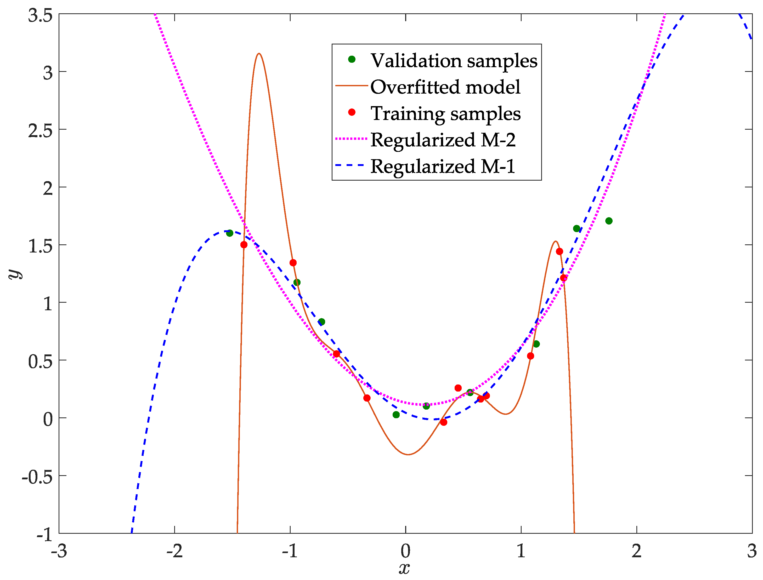
6.1. SOS Constrained Regression versus Regularization

The purpose of this simple example is to demonstrate the improved features of our physics-based regression approach w.r.t. the “blind” regularization summarized in Section 3.3.
Assume that a dataset of 20 samples is collected from an ill-known SISO process, and that a polynomial model for it is to be sought. For building such model, the data is randomly divided in two sets, { X T , Y T } with 11 samples for training and { X V , Y V } with the rest for validation:
X T = [ 0.6978 , 1.0811 , 0.5991 , 0.648 , 0.3354 , 1.3677 , 1.3317 , 0.9742 , 0.4538 , 0.329 , 1.4 ] , Y T = [ 0.1917 , 0.5362 , 0.554 , 0.1629 , 0.1718 , 1.2121 , 1.4415 , 1.3438 , 0.2583 , 0.0378 , 1.5 ] , X V = [ 1.4798 , 0.9409 , 0.7277 , 1.5231 , 1.7593 , 1.13 , 0.0821 , 0.5573 , 0.1789 ] , Y V = [ 1.64 , 1.173 , 0.8318 , 1.6 , 1.706 , 0.64 , 0.027 , 0.2193 , 0.1025 ] .
Looking at the plotted data in Figure 2, one may infer that the “obscure” process could be convex, so fitting with quadratic candidate models would be satisfactory enough. However, this is not the case as we will explain later, and note that this visual inspection would not be possible in high-dimensional systems. Therefore, for the shake of better fitness, the candidate model will be a polynomial of, at most, degree d = 8 :
p ( c , x ) = c 0 + c 1 x + c 2 x 2 + c 3 x 3 + c 4 x 4 + c 5 x 5 + c 6 x 6 + c 7 x 7 + c 8 x 8 .
As expected, using classical unconstrained LS with (20) and just 11 samples for training leads to a totally useless overfitted model (orange curve in Figure 2) with two local minima and drastically falling down around | x | 1 . 5 .

6.1.1. Least Squares with Regularization

In order to avoid overfitting, regularization in c is recalled (Section 3.3). In this approach, the user must set the metaparameter Γ a priori and then perform an exploration in γ to find the best fitting for such Γ . This means that the performance in this approach is very tailored to have a good guess for Γ . Unfortunately, the metaparameter cannot be easily related to any physical insight, but only to reduce the influence of some non-preferred monomials, normally the higher-degree ones. Following this idea, two typical alternatives for the metaparameter were tested:
[ M 1 ] Γ = [ 0 , 0 , 0 , 1 , 1 , 10 , 10 , 100 , 100 ] T ; [ M 2 ] Γ = [ 0 , 0 , 1 , e 2 , e 3 , e 4 , e 5 , e 6 , e 7 ] T .
Note that coefficients of the zero-order and linear terms are not penalized in both alternatives (at least the best linear prediction will be found in the worst case). Moreover, the quadratic term is also freed due to such intuition of convexity from data visual inspection, whereas the higher-order monomials are progressively penalized. In M-2, the usual exponential penalty with the monomials degree is set in order to balance fitness to data with model complexity.
After exploration in γ for both setups, the model with less total fitting error (chosen to be training plus validation errors) is found at γ = 0.4 with the chosen exploration granularity. The best model (coefficients below c < 10 4 are disregarded) obtained with the metaparameter choice [M-1] is a polynomial of degree 7 (dashed blue curve in Figure 2), whereas [M-2] is a polynomial of degree 5 (dotted pink curve in Figure 2). Table 1 gives the fitting error for these “best” models, as well as some values resulting from the exploration in the regularization scaling parameter g a m m a .
Remark 2.
Looking at Figure 2, the model obtained by the usual exponential regularization [M-2] is preferable to the one obtained by the ad hoc [M-1] because it is quite symmetric and convex (at least in the depicted region), so it would be more “reliable” a priori for extrapolation in X : = { x : 2 < | x | < 3 } . However, note that simple visual inspection is not available for high-dimensional systems. Thus, without visual information, one would have chosen the model by [M-1], as it is the one which best fit the data.

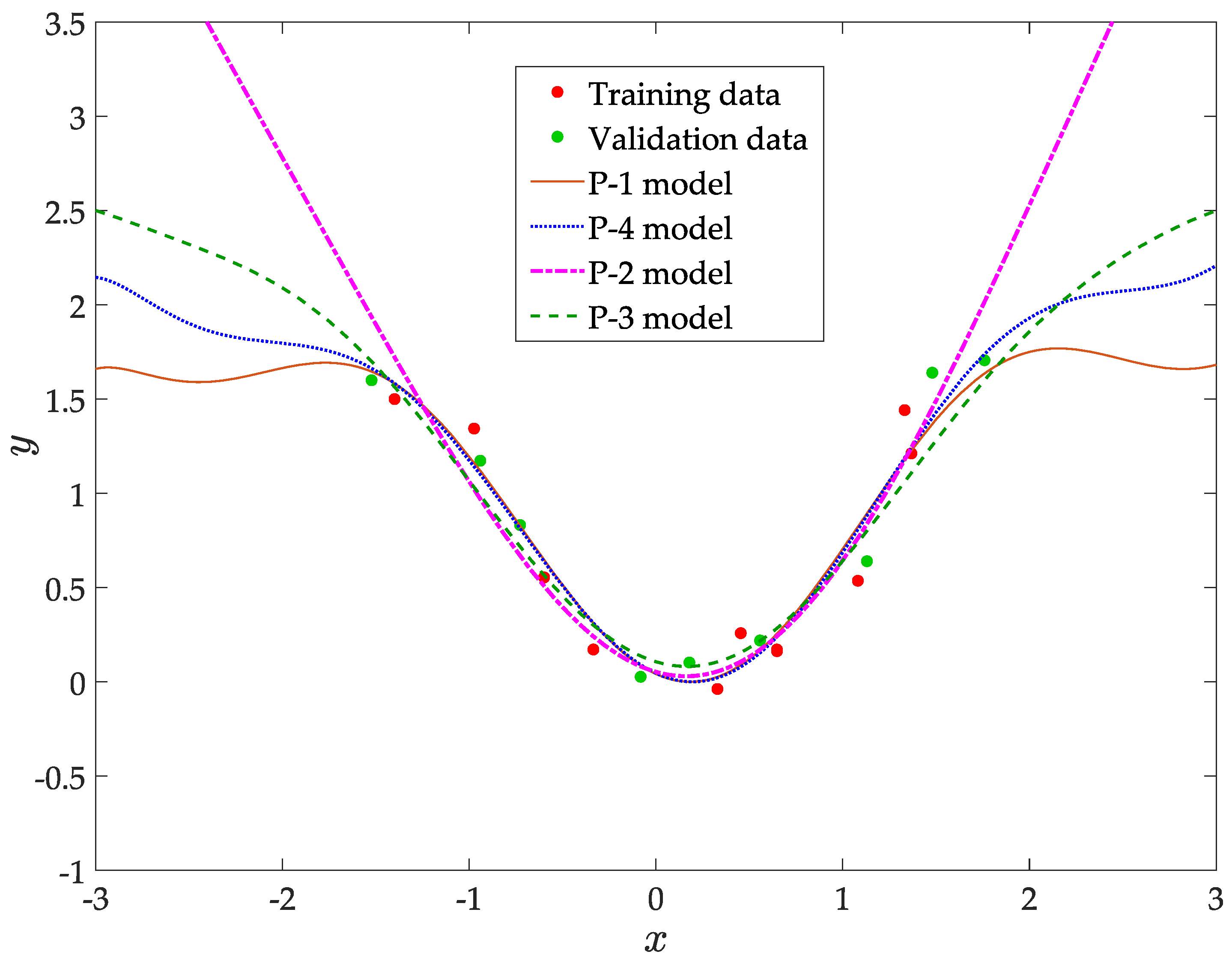
6.1.2. SOS Constrained Regression

Alternatively to the “blind” regularization, some desired features with physical insight on the model response could have been searched. Thus, as an initial idea, non-negativity and convexity were forced on (20) via SOS constrained regression (LS objective, Section 5) with the following constraints:
p ( c , x ) = c 0 + c 1 x + c 2 x 2 + c 3 x 3 + c 4 x 4 + c 5 x 5 + c 6 x 6 + c 7 x 7 + c 8 x 8 Σ x ,
d 2 p ( c , x ) d x 2 = 2 c 2 + 6 c 3 x + 12 c 4 x 2 + 20 c 5 x 3 + 30 c 6 x 4 + 42 c 7 x 5 + 56 c 8 x 6 Σ x .
The convex polynomial found to best fit the training data ( E = 0.226 ) incurs in a high error on the validation data ( E = 14.46 ). By inspecting the modeling error with the data points (visual inspection omitted, as this possibility is hardly available in models with multiple inputs) it was found that the highest deviations appear mainly around the boundaries of the training region. Thence, it might be inferred that the generating process flattens far away from the origin, so it is probably nonconvex (or not strongly convex at least).
A simple way to find a model whose response fits better with this insight of flatness in extrapolation is to set up local upper and lower bounds on p ( c , x ) : y ¯ p ( c , x ) 0 x { x : | x | < 3 } ; p ( c , x ) y ̲ 0 x { x : 2 < | x | < 3 } or better by locally bounding the slope to small values in ψ : = { x : 2 < | x | < 3 } . Using Lemma 1, this last condition is enforced by the following SOS constraints:
p ( c , x ) s 1 ( a 1 , x ) · ( 3 2 x 2 ) Σ x , 0 . 3 d p ( c , x ) d x s 2 ( a 2 , x ) · ( 3 2 x 2 ) s 3 ( a 3 , x ) · ( x 2 2 ) Σ x , d p ( c , x ) d x + 0 . 3 s 4 ( a 4 , x ) · ( 3 2 x 2 ) s 5 ( a 5 , x ) · ( x 2 2 ) Σ x ,
with s i ( a i , x ) Σ x being SOS polynomial multipliers whose highest degree is d 6 , as p ( c , x ) can be of degree 8. Note that local non-negativity of p on X : = { x : | x | < 3 } is also enforced, as there is no need to force global positivity outside the region considered for extrapolation, thus reducing conservatism.
The model obtained with this approach is the solid orange curve in Figure 3, labelled as [P-1]. This desired response was obtained with a total regression error (training plus validation) of E = 0.41 , beating by 25% the best fit obtained by the regularization approach.
Nonetheless, the response shows several local minima in X . If this surrogate model is to be integrated in a larger grey-box model for real-time optimization purposes, getting a quasi-monotonous model (single global minimum) could be more interesting than achieving the lowest fitting error, in order to reduce the probability of getting stuck in local optima with gradient-based NLP solvers. Several alternative ways are available to handle this issue via SOS constrained regression:
[P-2] 
Positive curvature in X , tending to zero when x ψ (dashed-dotted pink curve in Figure 3):
p ( c , x ) 0 , d 2 p ( c , x ) d x 2 0 , x X ; d 2 p ( c , x ) d x 2 0.25 x ψ ,
[P-3] 
Upper bound on p in X and bounded negative curvature in x ψ (dashed green curve):
2.5 p ( c , x ) 0 x X ; 0 d 2 p ( c , x ) d x 2 > 0.8 x ψ ,
[P-4] 
Symmetrically bounding the slope between two values in x ψ (dotted blue curve):
p ( c , x ) 0 x X ; 0 . 1 < d p ( c , x ) d x < 0 . 6 x { 2 x 3 } ; 0 . 1 d p ( c , x ) d x 0 . 6 x { 2 x 3 } .
As can be seen in Figure 3, the three approaches (P-2 to P-4) get quasi-monotonous surrogate models which are suitable for optimization purposes. The total regression error is quite similar in all the approaches (Table 2) and the small differences between them could be just a product of sheer luck (fitting the sensor noise). Thus, the choice of one over the other would only depend on the engineer physical intuition.
Remark 3.
Note that the standard LS regularization was not able to find these more feasible models obtained with the SOS approach, at least with the tested values for the metaparameter Γ. Anyway, although it may be found, there is no clear and direct relation between Γ and the features desired in the model response.

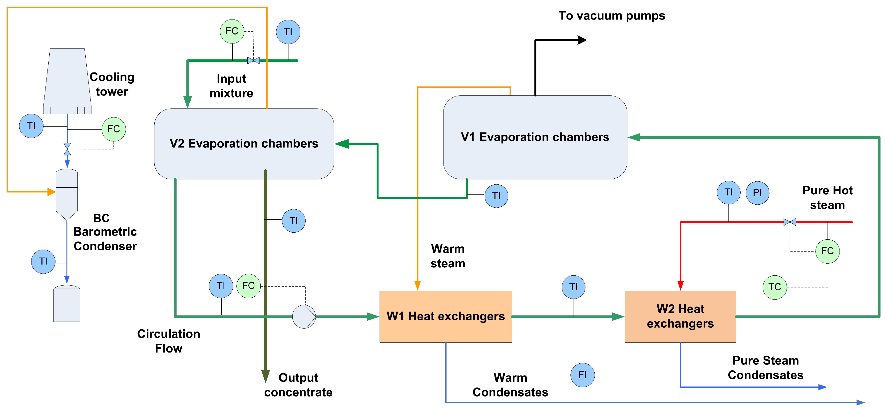
6.2. Modeling the Heat-Transfer in an Evaporation Plant

In this example, we make use of the proposed methodology in Section 4 to build up a grey-box model for a multiple-effect evaporation plant of a man-made cellulose fiber production factory.
The plant is formed by several evaporation chambers and some heat exchangers in serial connection, a mixing steam condenser and a cooling tower, forming a multiple-effect evaporation system. See Figure 4, where individual equipment have been lumped together for confidentiality reasons and due to the lack of measurements in between. The plant receives a liquid input, mixture of water with chemical components and leftovers of organic material. The goal is to concentrate the liquid by removing a certain amount of water.
The process operates as follows: the liquid enters the system by chamber V 2 and then goes sequentially through the sets of heat exchangers W 1 and W 2 to increase its temperature up to a desired setpoint. In W 1 , the temperature rise is achieved from saturated-steam flows recirculated from the evaporation chambers V 1 . Then, the temperature setpoint is reached in W 2 thanks to a fresh steam inlet from boilers. Afterwards, the hot liquid enters sequentially into the low-pressure set of chambers V 1 , where a partial evaporation of water takes place. The remaining evaporation is achieved in the last chambers V 2 thanks to the pressure drop in the mixing condenser B C , linked to the cooling tower. Finally, part of the concentrated solution leaves the plant by V 2 and the rest mixes again with the inlet, being recirculated to the heat exchangers.

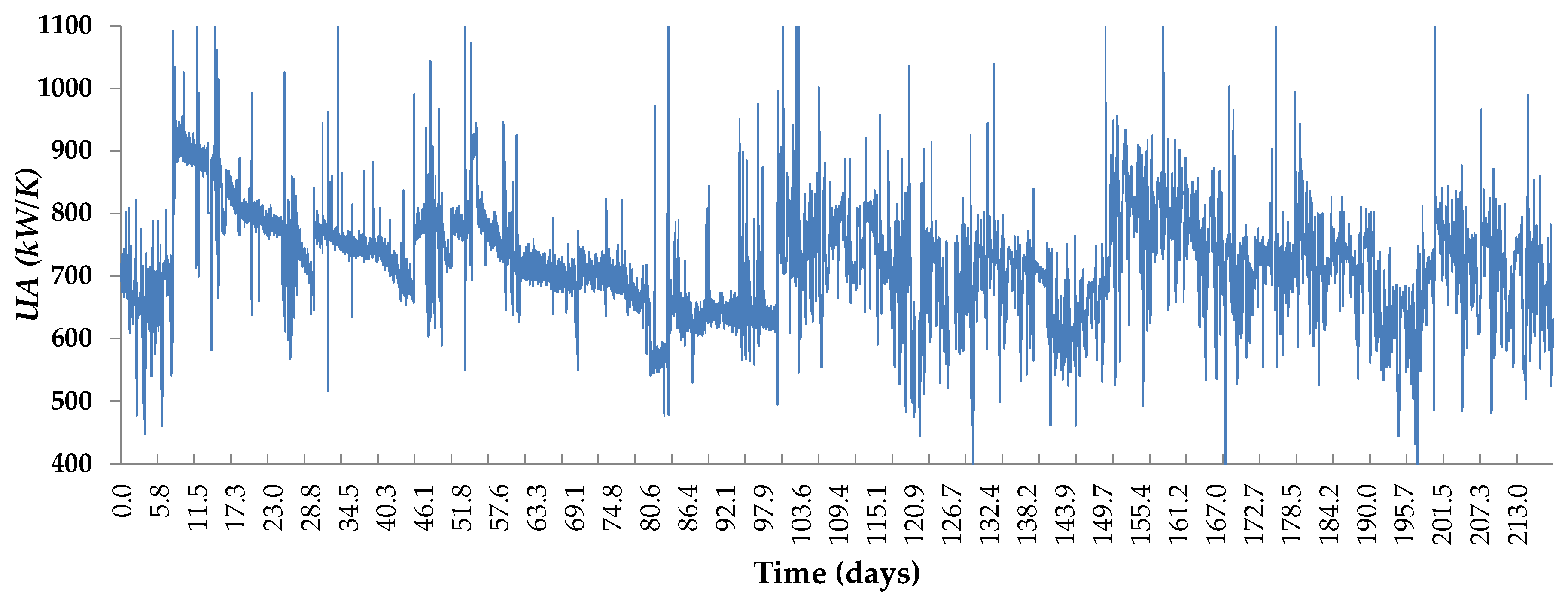
6.2.1. Stage 1: Estimation

Our modeling approach starts from a nonlinear set of equations of the plant in steady state, obtained from first principles. These equations have been omitted here for brevity, but the reader is referred to the previous works of the authors [45,46] to get a detailed description of both the plant and the physical model equations. Then, in the estimation phase (Stage 1 of the proposed methodology), DR is performed to “clean” the process data from incoherent sensor values and to get suitable estimates for the internal-model variables and time-varying parameters, in particular for the average heat-transfer coefficient U A ( t ) in the lumped heat exchangers. Note that this time-varying parameter depends on the conduction and convection effects plus the exchange surface, values that are not precisely known or complex to model.
Here, the focus is on U A because an accurate modeling of the long-term fouling dynamics in the heat-exchangers pipes is key for a realistic optimization of the operation, and the right scheduling of the maintenance tasks. Indeed, this issue is shared with other industrial systems like furnaces or catalyst deactivation in chemical reactors. All have in common a system-efficiency degradation, which may be palliated or worsened by the way the equipment operates.
Thus, a set of experiments were performed on site, running the plant in different operating conditions (setting different values for the main control variables: the circulation flow and the temperature setpoint). Moreover, in order to get significant information from the actual fouling process, the plant historian for several months of operation (including some stops for cleaning) has been also provided as experimental data for reconciliation. Figure 5 shows the estimated U A for exchangers W 1 , provided by the DR (details omitted for brevity).

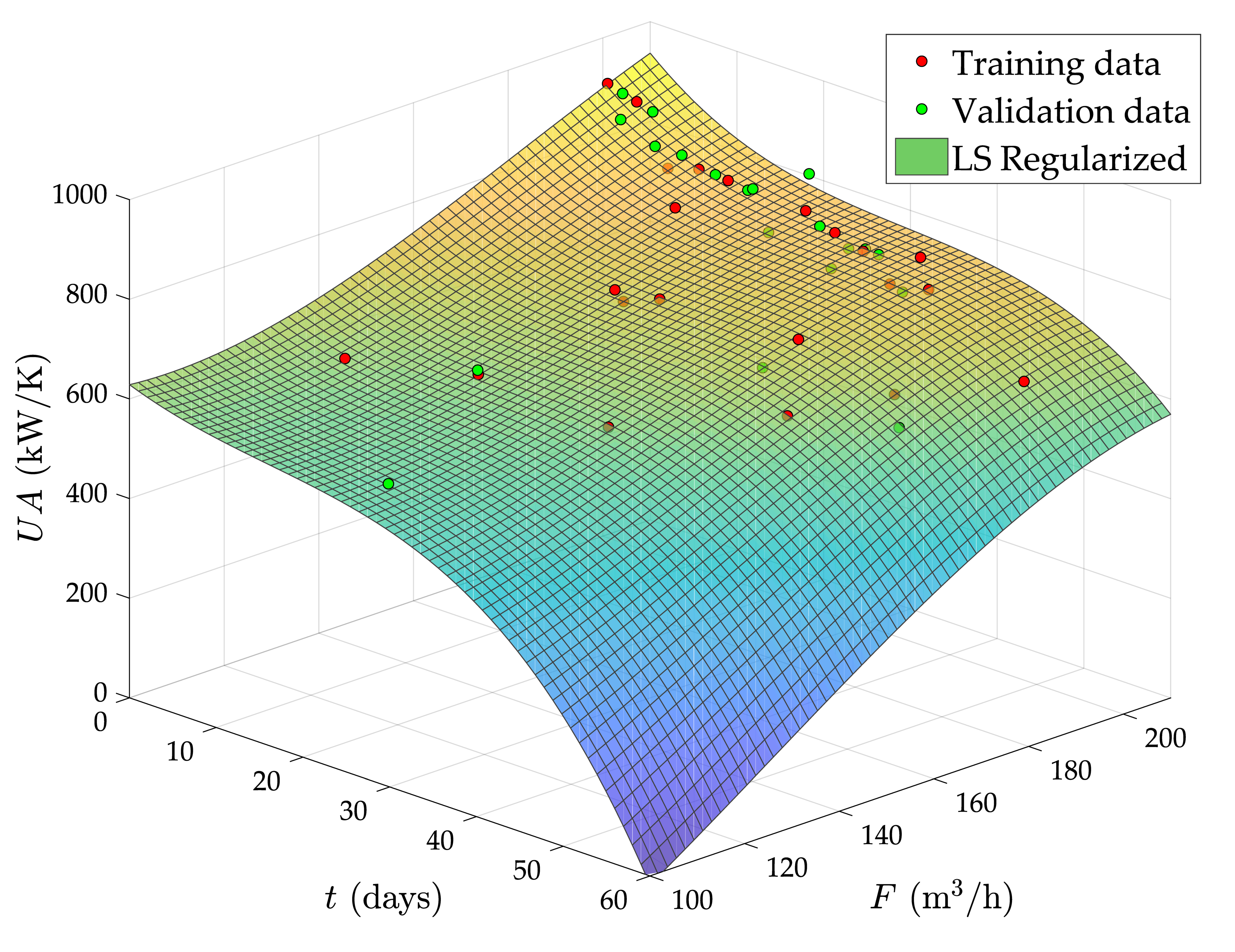
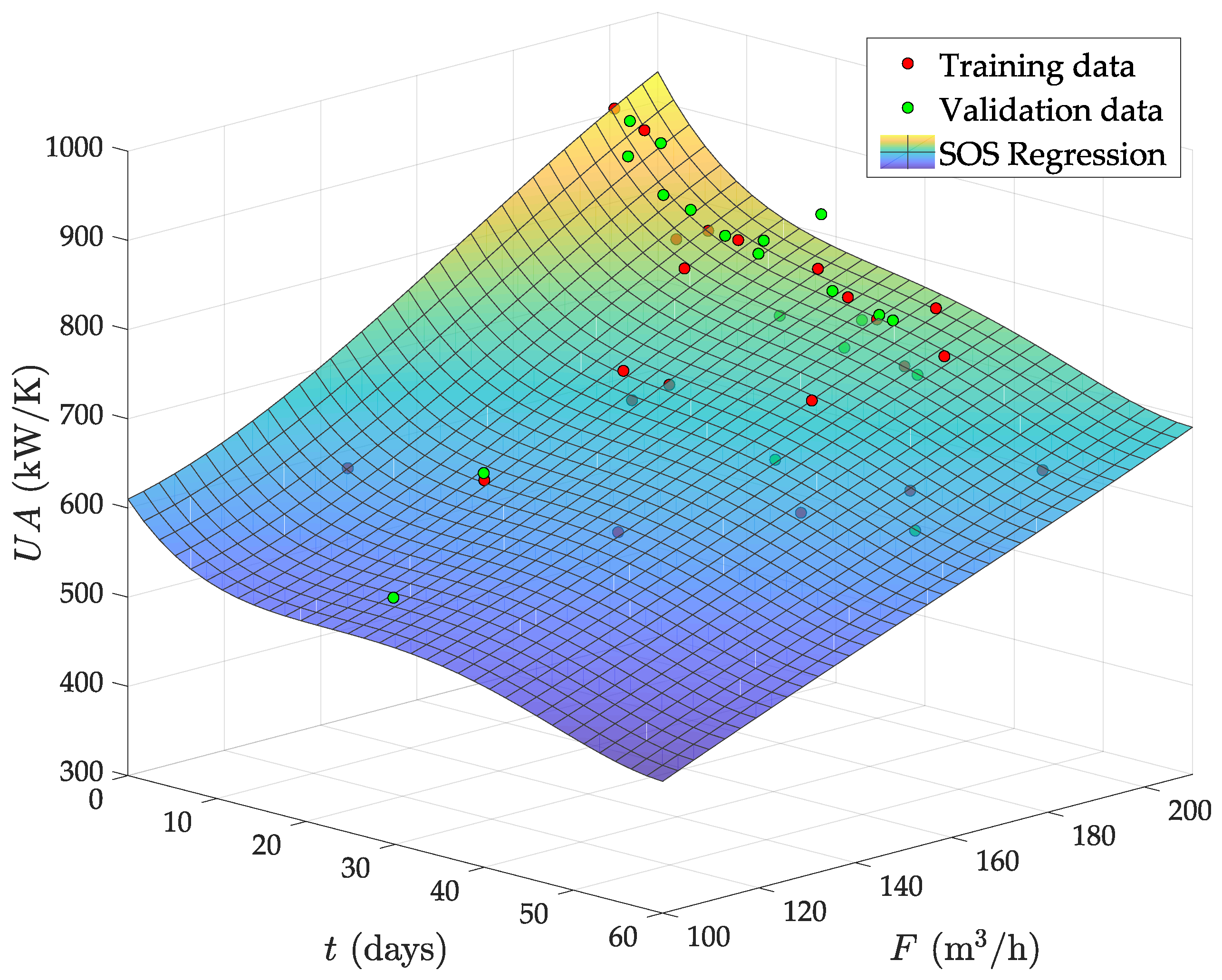
6.2.2. Stage 2: Regression

The objective now in the regression stage is to build up a polynomial regression model U A = p ( c , F , t ) to link/predict the heat-transfer coefficient U A with the circulating flow through the exchangers F and with the time t that the plant is in operation since last cleaning.
The first issue arises when selecting the samples for training and validation. Although the recorded dataset of seven months with a sampling time of 5 min may look huge, the quality of data is much more important that the quantity of samples. In addition, in this case, the plant was usually working at high circulating flows, except in the few experiments executed on purpose and in particular situations (product changeovers). Therefore, lots of data for the plant operating in a local region are available, but a significant amount of information of the convection and fouling behaviors at medium/low flows is missing.
Note importantly that, although there is no major computational issue in performing regularized or SOS constrained regression with hundreds of data, if lots of such data are agglomerated around the same operating point, the fitted model might specialize too much in such region, as the model structure for regression will not likely contain the same nonlinearities as the actual plant which generated the data. Hence, the prediction capabilities out of this region can be seriously compromised with such a model. Therefore, the data points must be “triaged” according to their degree of uniqueness (data containing almost-redundant information should get lower weights in the regression problem, or be directly removed from the training set) in order to prevent this possible model bias due to strong non-uniform data densities.
Consequently, after inspecting and analyzing the plant historian, we ended up with a selected subset of 22 samples ( U A , F , t ) for training plus 20 samples for validation. These data, depicted in Figure 6, contains nearly all the information available in the feasible region of operation:
Ω : = { F , t R + : 100 F 200 m 3 / h , t 60 days } .
As it can be observed by simple visual inspection, there are many samples covering Ω at high flows, but there is a significant lack of information at lower flows, especially when the plant works after cleaning and when it is in operation for more than 40 days.
After normalizing these data to zero mean and σ = 1 , a standard LS identification was initially tested with exponential regularization in the coefficients corresponding to the higher-degree monomials of p ( c , F , t ) , analogous to M-2 in the previous example. Thus, after exploring in γ , the best fitting (lower total error) is achieved with a polynomial of coordinate degree at most d = 3 ( γ = 0.025 ):
U A ( F , t ) = 2 . 5335 · 10 4 F 3 7 . 0692 · 10 4 F 2 t + 2 . 0131 · 10 3 F t 2 5 . 5415 · 10 3 t 3 + 0 . 13823 F 2 + 0 . 14058 F t + 0 . 066824 t 2 21 . 0228 F 13 . 8979 t + 1602 . 0089 .
Independently of the fitting error (shown in Table 3), there are two aspects in this model which are unacceptable:
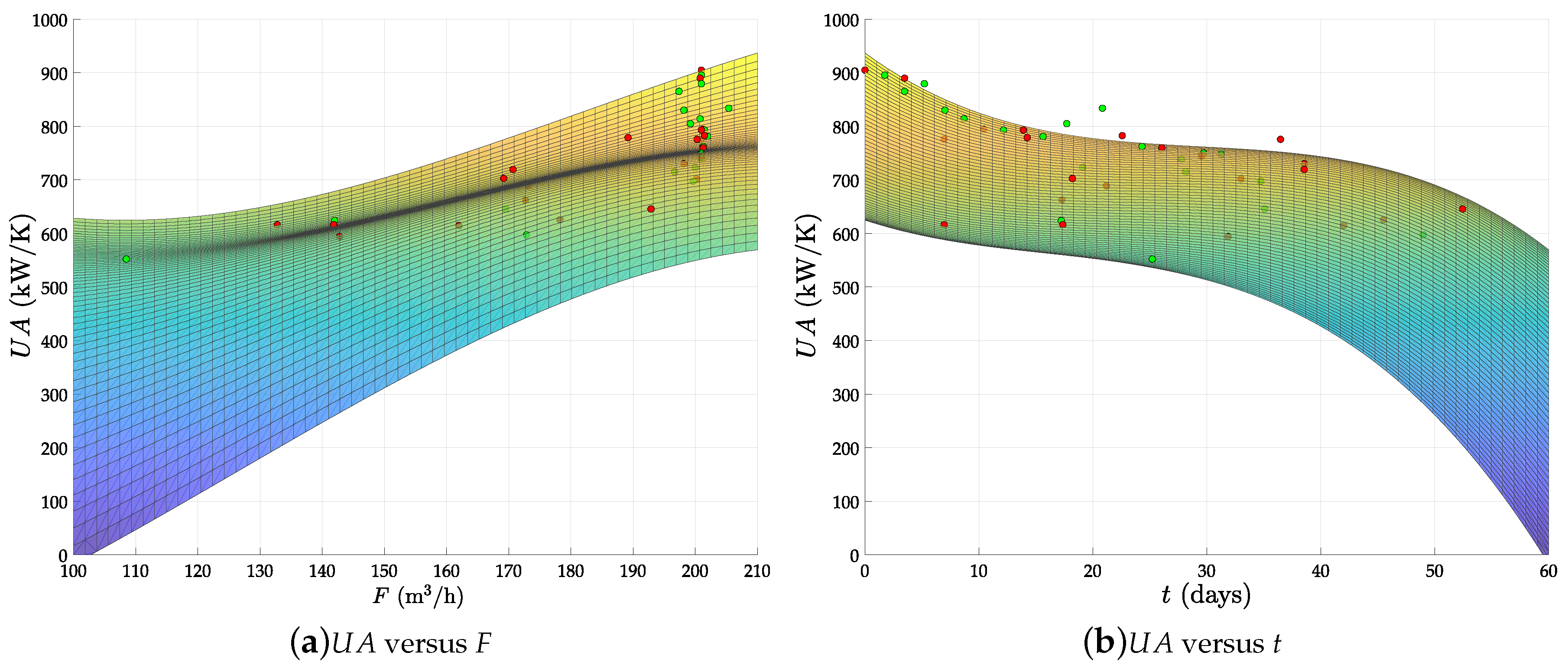
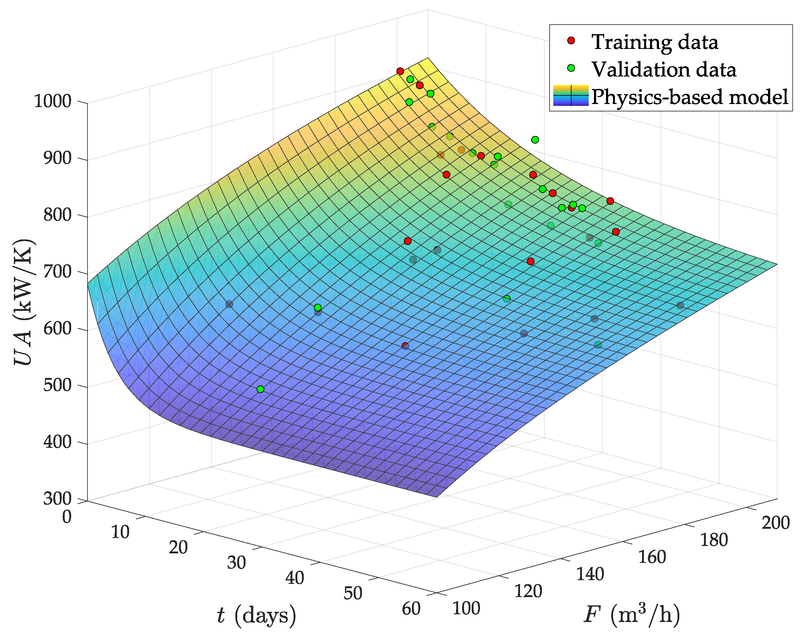
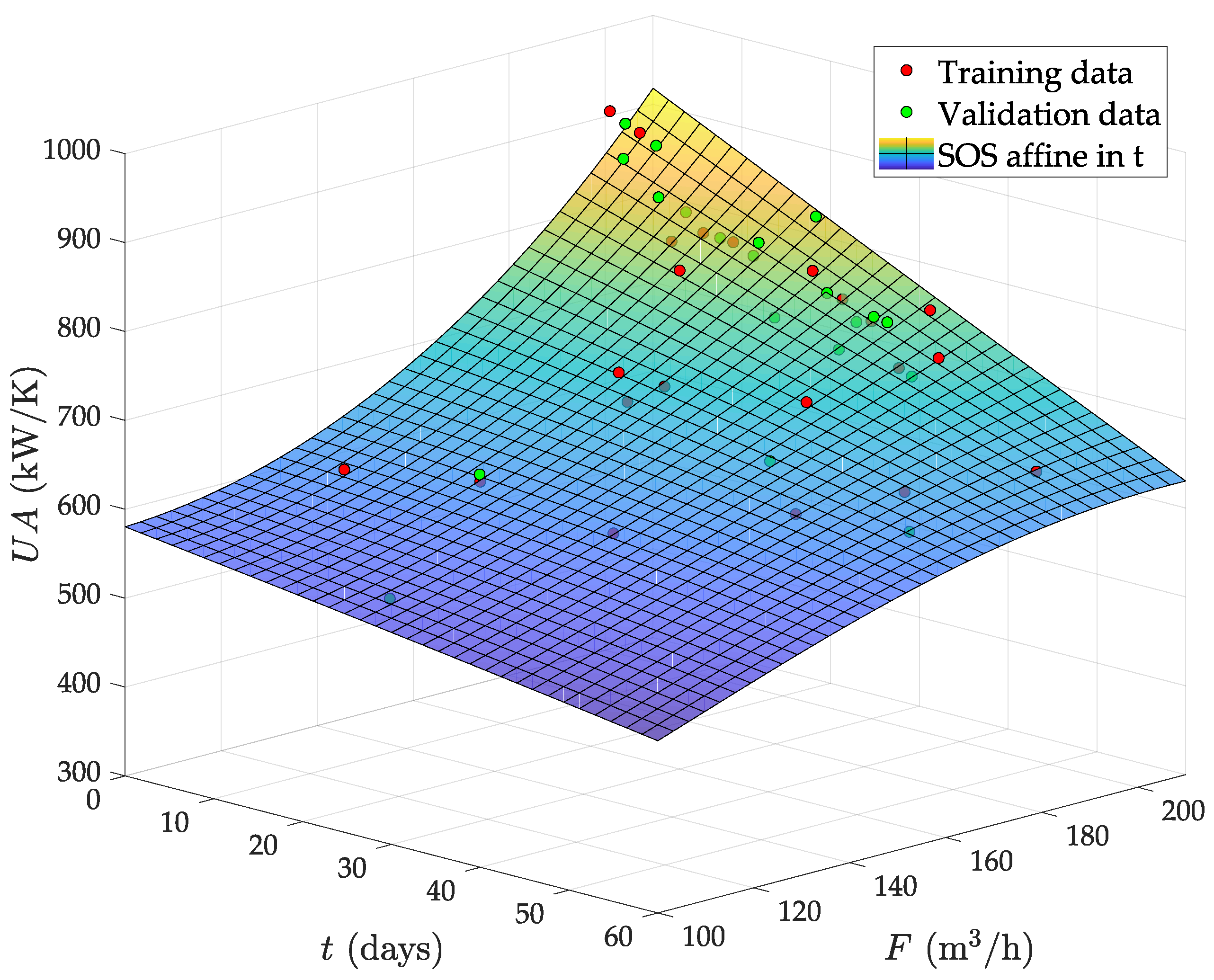
  • The circulating flow is fixed by a pump in this plant. Therefore, the fouling due to deposition of organic material must tend to a saturation limit with the time. This is because the flow speed increases as the effective pipe area reduces by fouling and, from basic physics, the deposition of particles in the pipes must always decrease with the flow speed. Therefore, the abrupt falling of the U A from day 30 onwards is not possible. Indeed, the predicted U A even reaches zero and negative values after two months of operation with low F.
  • With a nearly constant exchange area, U A always decreases as F does, by convective thermodynamics. Hence, the mild increase observed at low F when the evaporator is fully clean (see Figure 7a) is also physically impossible.
Now, SOS constrained regression in Section 5 is recalled to incorporate the above physical requirements in the identification problem. Hence, regularization in the model coefficients is removed but, instead, the following constraints are added:
d p ( c , F , t ) d t < 0 , d p ( c , F , t ) d F > 0 F , t Ω ,
d p ( c , F , t ) d t > λ t , d p ( c , F , t ) d F < λ F F , t Ω { t : 30 < t < 60 } , λ t , λ F R + ,
with λ t , λ F , being user-defined bounds on the model slopes that are set up to force the expected nearly-flat response in U A after a month of operation.
Performing the change of variables in ( F , t ) corresponding to the normalized data, and casting (26) and (27) to SOS constraints, locally enforced in the corresponding regions via multipliers s i ( a i , F , t ) Σ F , t with highest degree d = 2 , the model which best fit the experimental data ( λ t = λ F = 0.6 are set for regression, as the input data for both F and t are normalized) is found to be a polynomial of d = 4 :
U A ( F , t ) = 7 . 0667 · 10 8 F 4 + 2 . 9544 · 10 6 F 3 t + 1 . 6325 · 10 6 F 2 t 2 2 . 4195 · 10 6 F t 3 + 1 . 0012 · 10 4 t 4 1 . 9868 · 10 4 F 3 1 . 5847 · 10 3 F 2 t + 5 . 0898 · 10 5 F t 2 0 . 013865 t 3 + 0 . 088883 F 2 + 0 . 23223 F t + 0 . 62707 t 2 10 . 8758 F 22 . 7836 t + 1000 . 2034 .
Figure 8 shows how the model (28) behaves more coherent with the process physics, and just with an ~1.3% of relative fitness deterioration with respect to the LS-regularized model (25) (see Table 3).

6.2.3. Comparison with Previous Works

In the previous work [45], we followed the typical grey-box modeling approach of setting up a functional form for U A ( F , t ) and then solving an unconstrained LS-optimization problem. This was a quite time-consuming task, though we arrived to satisfactory enough results with the physically-based functional model:
U A ( F , t ) = U A 0 k 1 F 1 / 3 k 2 e 1 τ F 2 t , U A 0 , k 1 , k 2 , τ R + .
The best fitting of (29) to the selected experimental data ( U A 0 = 1744.5 , k 1 = 4928.1 , k 2 = 214.64 and τ = 2096.3 ), here with no distinction between training and validation sets as the model structure is fully fixed, gives us a quite desirable response (see Figure 9). However, the fitting to the experimental data degrades in ~25% w.r.t. model (28).
Furthermore, in [10], we assumed the hypothesis that the increase of specific-steam consumption in the plant due to fouling was linear with the operation time. This was done based on direct measurements and to facilitate the resolution of the maintenance-scheduling problem formulated in [10]. Now, we analyze whether this assumption was reasonably true.
For this aim, the polynomial model p ( c , F , t ) is forced to be affine in t. This requirement can be easily achieved by adding the following constraint on the curvature to the SOS regression problem:
d 2 p ( c , F , t ) d t 2 = 0 F , t Ω ,
which can be cast as an SOS equality constraint and checked locally in Ω via Lemma 1. Doing this, effectively the obtained model is affine in t and nonlinear in F, as Figure 10 shows.
This model also incurs in an ~20% fitting degradation w.r.t. the optimal (28). In this case, what is more relevant than the fitting error is the observed variation of the slope in t at different flows. This indicates that the assumption in [10] was acceptable as long as F remains nearly constant. Indeed, as the plant was normally operating at high flows when the data was collected from the plant historian, we did (could) not realize of this varying behavior with the flow.

7. Discussion

The above examples show how high-degree polynomials with well-behaved output can be obtained via SOS-constrained regression even in the presence of scarce measurements, though there is no major issue in using larger datasets, especially with the economic singular-value decomposition (12). Indeed, the main computational effort with SOS programming is employed in casting the SOS polynomial constraints as SDP ones, not in the number of samples to fit in the objective function.
The average computational time (Intel® i7-4510U machine) required to solve the SOS-constrained regression problems in Section 6.2 is 1.5 s (calling the SDP solver SeDuMi), whereas the nonlinear unconstrained LS regression in Section 6.2.3 needs 0.15 s (using the NLP solver IPOPT with MUMPS as linear solver). Hence, at the price of this increase in the computational demands, the modeler is allowed to naturally include the physical insight into the regression problem via (polynomial) bounds on value, slope and curvature or convexity-related constraints, thus getting coherent model responses.
Note also that the proposed SOS-constrained regression can be an alternative to standard regularization, but both can also be complementary if desired because there is no impediment in weighting the coefficients of the regression model with some metaparameter Γ , whereas, at the same time, some polynomial constraints are to be enforced. In fact, if Γ is chosen according to some information criteria, this combined approach might provide an automatic selection of the suitable model structure by balancing the fitness to data with the model complexity. This possibility will be explored for further works.
The two-stage methodology for grey-box modeling proposed in Section 4, enhanced with the application of SOS-constrained regression (Section 5), has demonstrated its advantages to face a modeling problem for optimization purposes in a real industrial evaporation plant. The main limitation of the approach is that candidate regression submodels are limited to being polynomials, though polynomial basis functions are flexible, used in practice, and the dominant process nonlinearities are taken into account in the first-principles equations. Nevertheless, the possible extension of the SOS-regression approach to include other non-polynomial basis functions will be explored via multimodel and polynomial bounding.
As a final remark, note that, although SOS programming is convex optimization and the proposed methodology is performed offline, its scalability is mainly limited by the number of independent variables in x and by the degree of the involved polynomials d. This fact may pose limitation in applying the proposed ideas to perform regression in complex chemical-reaction problems with many components involved. Nonetheless, the ALAMO approach does not get clear computational benefits in this sense either. Moreover, it is worth noting that the main aim of the SOS approach is not to get complete-plant surrogate models (though they can be sought at relatively small process scales), but just local relationships among a few process variables to complete a grey-box model based on physics.

Author Contributions

Conceptualization, J.L.P. and C.d.P.; methodology, J.L.P. and C.d.P.; software, J.L.P.; validation, J.L.P. and A.S.; formal analysis, A.S.; investigation J.L.P. and A.S.; resources, C.d.P.; writing–original draft preparation, J.L.P.; writing–review and editing, A.S.; visualization, J.L.P.; supervision, A.S. and C.d.P.; project administration, C.d.P.; funding acquisition, C.d.P.

Funding

This research received funding from the European Union, Horizon 2020 research and innovation programme under Grant No. 723575 (CoPro), and from the EU plus the Spanish Ministry of Economy, grant DPI2016-81002-R (AEI/FEDER).

Acknowledgments

The authors especially thank the industrial partner Lenzing AG (Lenzing, Austria) for the data acquisition and experimental tests carried out in the evaporation plant.

Conflicts of Interest

The authors declare no conflict of interest. The funders had no role in the design of the study; in the collection, analysis, or interpretation of data; in the writing of the manuscript, or in the decision to publish the results.

References

  1. Davies, R. Industry 4.0: Digitalization for Productivity and Growth; Document pe 568.337; European Parliamentary Research Service: Brussels, Belgium, 2015. [Google Scholar]
  2. Krämer, S.; Engell, S. Resource Efficiency of Processing Plants: Monitoring and Improvement; John Wiley & Sons: Weinheim, Germany, 2017. [Google Scholar]
  3. Palacín, C.G.; Pitarch, J.L.; Jasch, C.; Méndez, C.A.; de Prada, C. Robust integrated production-maintenance scheduling for an evaporation network. Comput. Chem. Eng. 2018, 110, 140–151. [Google Scholar] [CrossRef]
  4. Maxeiner, L.S.; Wenzel, S.; Engell, S. Price-based coordination of interconnected systems with access to external markets. Comput. Aided Chem. Eng. 2018, 44, 877–882. [Google Scholar]
  5. Afram, A.; Janabi-Sharifi, F. Black-box modeling of residential HVAC system and comparison of gray-box and black-box modeling methods. Energy Build. 2015, 94, 121–149. [Google Scholar] [CrossRef]
  6. Witten, I.H.; Frank, E.; Hall, M.A.; Pal, C.J. Data Mining: Practical Machine Learning Tools and Techniques; Morgan Kaufmann: San Francisco, CA, USA, 2016. [Google Scholar]
  7. Olsen, I.; Endrestøl, G.O.; Sira, T. A rigorous and efficient distillation column model for engineering and training simulators. Comput. Chem. Eng. 1997, 21, S193–S198. [Google Scholar] [CrossRef]
  8. Galan, A.; de Prada, C.; Gutierrez, G.; Sarabia, D.; Gonzalez, R. Predictive Simulation Applied to Refinery Hydrogen Networks for Operators’ Decision Support. In Proceedings of the 12th IFAC Symposium on Dynamics and Control of Process Systems, Including Biosystems (DYCOPS), Florianópolis, Brazil, 23–26 April 2019. [Google Scholar]
  9. Kar, A.K. A hybrid group decision support system for supplier selection using analytic hierarchy process, fuzzy set theory and neural network. J. Comput. Sci. 2015, 6, 23–33. [Google Scholar] [CrossRef]
  10. Kalliski, M.; Pitarch, J.L.; Jasch, C.; de Prada, C. Apoyo a la Toma de Decisión en una Red de Evaporadores Industriales. Revista Iberoamericana de Automática e Informática Industrial 2019, 16, 26–35. [Google Scholar] [CrossRef]
  11. Zorzetto, L.; Filho, R.; Wolf-Maciel, M. Processing modelling development through artificial neural networks and hybrid models. Comput. Chem. Eng. 2000, 24, 1355–1360. [Google Scholar] [CrossRef]
  12. Cellier, F.E.; Greifeneder, J. Continuous System Modeling; Springer Science & Business Media: New York, NY, USA, 2013. [Google Scholar]
  13. Zou, W.; Li, C.; Zhang, N. A T–S Fuzzy Model Identification Approach Based on a Modified Inter Type-2 FRCM Algorithm. IEEE Trans. Fuzzy Syst. 2018, 26, 1104–1113. [Google Scholar] [CrossRef]
  14. Neumaier, A. Solving Ill-Conditioned and Singular Linear Systems: A Tutorial on Regularization. SIAM Rev. 1998, 40, 636–666. [Google Scholar] [CrossRef] [Green Version]
  15. Kim, S.; Koh, K.; Lustig, M.; Boyd, S.; Gorinevsky, D. An Interior-Point Method for Large-Scale 1-Regularized Least Squares. IEEE J. Sel. Top. Signal Process. 2007, 1, 606–617. [Google Scholar] [CrossRef]
  16. Llanos, C.E.; Sanchéz, M.C.; Maronna, R.A. Robust Estimators for Data Reconciliation. Ind. Eng. Chem. Res. 2015, 54, 5096–5105. [Google Scholar] [CrossRef]
  17. de Prada, C.; Hose, D.; Gutierrez, G.; Pitarch, J.L. Developing Grey-box Dynamic Process Models. IFAC-PapersOnLine 2018, 51, 523–528. [Google Scholar] [CrossRef]
  18. Cozad, A.; Sahinidis, N.V.; Miller, D.C. A combined first-principles and data-driven approach to model building. Comput. Chem. Eng. 2015, 73, 116–127. [Google Scholar] [CrossRef]
  19. Cozad, A.; Sahinidis, N.V. A global MINLP approach to symbolic regression. Math. Programm. 2018, 170, 97–119. [Google Scholar] [CrossRef]
  20. Reemtsen, R.; Rückmann, J.J. Semi-Infinite Programming; Springer Science & Business Media: New York, NY, USA, 1998; Volume 25. [Google Scholar]
  21. Parrilo, P.A. Semidefinite programming relaxations for semialgebraic problems. Math. Programm. 2003, 96, 293–320. [Google Scholar] [CrossRef] [Green Version]
  22. Nauta, K.M.; Weiland, S.; Backx, A.C.P.M.; Jokic, A. Approximation of fast dynamics in kinetic networks using non-negative polynomials. In Proceedings of the 2007 IEEE International Conference on Control Applications, Singapore, 1–3 October 2007; pp. 1144–1149. [Google Scholar]
  23. Tan, K.; Li, Y. Grey-box model identification via evolutionary computing. Control Eng. Pract. 2002, 10, 673–684. [Google Scholar] [CrossRef] [Green Version]
  24. Biegler, L.T. Nonlinear Programming: Concepts, Algorithms, and Applications to Chemical Processes; MOS-SIAM Series on Optimization: Philadelphia, PA, USA, 2010; Volume 10. [Google Scholar]
  25. Schuster, A.; Kozek, M.; Voglauer, B.; Voigt, A. Grey-box modelling of a viscose-fibre drying process. Math. Comput. Model. Dyn. Syst. 2012, 18, 307–325. [Google Scholar] [CrossRef]
  26. Tulleken, H.J. Grey-box modelling and identification using physical knowledge and bayesian techniques. Automatica 1993, 29, 285–308. [Google Scholar] [CrossRef]
  27. Leibman, M.J.; Edgar, T.F.; Lasdon, L.S. Efficient data reconciliation and estimation for dynamic processes using nonlinear programming techniques. Comput. Chem. Eng. 1992, 16, 963–986. [Google Scholar] [CrossRef]
  28. Bendig, M. Integration of Organic Rankine Cycles for Waste Heat Recovery in Industrial Processes. Ph.D. Thesis, Institut de Génie Mécanique, École Polytechnique Fédérale de Lausanne, Lausanne, Switzerland, 2015. [Google Scholar]
  29. Lasserre, J.B. Sufficient conditions for a real polynomial to be a sum of squares. Archiv der Mathematik 2007, 89, 390–398. [Google Scholar] [CrossRef] [Green Version]
  30. Parrilo, P.A. Structured Semidefinite Programs and Semialgebraic Geometry Methods in Robustness and Optimization. Ph.D. Thesis, California Institute of Technology, Pasadena, CA, USA, 2000. [Google Scholar]
  31. Papachristodoulou, A.; Anderson, J.; Valmorbida, G.; Prajna, S.; Seiler, P.; Parrilo, P. SOSTOOLS version 3.00 sum of squares optimization toolbox for MATLAB. arXiv, 2013; arXiv:1310.4716. [Google Scholar]
  32. Hilbert, D. Ueber die Darstellung definiter Formen als Summe von Formenquadraten. Mathematische Annalen 1888, 32, 342–350. [Google Scholar] [CrossRef]
  33. Scherer, C.W.; Hol, C.W.J. Matrix Sum-of-Squares Relaxations for Robust Semi-Definite Programs. Math. Programm. 2006, 107, 189–211. [Google Scholar] [CrossRef]
  34. Putinar, M. Positive Polynomials on Compact Semi-algebraic Sets. Indiana Univ. Math. J. 1993, 42, 969–984. [Google Scholar] [CrossRef]
  35. Pitarch, J.L. Contributions to Fuzzy Polynomial Techniques for Stability Analysis and Control. Ph.D. Thesis, Universitat Politècnica de València, Valencia, Spain, 2013. [Google Scholar]
  36. Scherer, C.; Weiland, S. Linear Matrix Inequalities in Control; Lecture Notes; Dutch Institute for Systems and Control: Delft, The Netherlands, 2000; Volume 3, p. 2. [Google Scholar]
  37. Wilson, Z.T.; Sahinidis, N.V. The ALAMO approach to machine learning. Comput. Chem. Eng. 2017, 106, 785–795. [Google Scholar] [CrossRef] [Green Version]
  38. Hindmarsh, A.C.; Brown, P.N.; Grant, K.E.; Lee, S.L.; Serban, R.; Shumaker, D.E.; Woodward, C.S. SUNDIALS: Suite of nonlinear and differential/algebraic equation solvers. ACM Trans. Math. Softw. (TOMS) 2005, 31, 363–396. [Google Scholar] [CrossRef]
  39. Gill, P.; Murray, W.; Saunders, M. SNOPT: An SQP Algorithm for Large-Scale Constrained Optimization. SIAM Rev. 2005, 47, 99–131. [Google Scholar] [CrossRef]
  40. Reynoso-Meza, G.; Sanchis, J.; Blasco, X.; Martínez, M. Design of Continuous Controllers Using a Multiobjective Differential Evolution Algorithm with Spherical Pruning. In Applications of Evolutionary Computation; Di Chio, C., Cagnoni, S., Cotta, C., Ebner, M., Ekárt, A., Esparcia-Alcazar, A.I., Goh, C.K., Merelo, J.J., Neri, F., Preuß, M., et al., Eds.; Springer: Berlin/Heidelberg, Germany, 2010; pp. 532–541. [Google Scholar]
  41. Andersson, J.; Åkesson, J.; Diehl, M. CasADi: A Symbolic Package for Automatic Differentiation and Optimal Control. In Recent Advances in Algorithmic Differentiation; Forth, S., Hovland, P., Phipps, E., Utke, J., Walther, A., Eds.; Springer: Berlin/Heidelberg, Germany, 2012; pp. 297–307. [Google Scholar]
  42. Hart, W.E.; Laird, C.D.; Watson, J.P.; Woodruff, D.L.; Hackebeil, G.A.; Nicholson, B.L.; Siirola, J.D. Pyomo—Optimization Modeling in Python; Springer Science & Business Media: New York, NY, USA, 2017; Volume 67. [Google Scholar]
  43. Wächter, A.; Biegler, L.T. On the implementation of an interior-point filter line-search algorithm for large-scale nonlinear programming. Math. Programm. 2006, 106, 25–57. [Google Scholar] [CrossRef]
  44. Sahinidis, N.V. BARON: A general purpose global optimization software package. J. Glob. Optim. 1996, 8, 201–205. [Google Scholar] [CrossRef]
  45. Pitarch, J.L.; Palacín, C.G.; de Prada, C.; Voglauer, B.; Seyfriedsberger, G. Optimisation of the Resource Efficiency in an Industrial Evaporation System. J. Process Control 2017, 56, 1–12. [Google Scholar] [CrossRef]
  46. Pitarch, J.L.; Palacín, C.G.; Merino, A.; de Prada, C. Optimal Operation of an Evaporation Process. In Modeling, Simulation and Optimization of Complex Processes HPSC 2015; Bock, H.G., Phu, H.X., Rannacher, R., Schlöder, J.P., Eds.; Springer International Publishing: Cham, Switzerland, 2017; pp. 189–203. [Google Scholar]
Figure 1. Standard DR scheme (decision variables highlighted in red).
Processes 07 00170 g001
Figure 2. Sampled data and polynomial models fitted by standard LS approaches.
Processes 07 00170 g002
Figure 3. Sampled data and polynomial models fitted by SOS constrained regression.
Processes 07 00170 g003
Figure 4. Simplified schema of the evaporation plant with existent instrumentation.
Processes 07 00170 g004
Figure 5. Estimated values of U A over seven months of operation.
Processes 07 00170 g005
Figure 6. Modeling U A through standard LS regularization.
Processes 07 00170 g006
Figure 7. Partial 2D views of the LS regularized model.
Processes 07 00170 g007
Figure 8. Modeling U A through SOS constrained regression.
Processes 07 00170 g008
Figure 9. Physics-based model for U A .
Processes 07 00170 g009
Figure 10. Polynomial affine-in-t model for U A .
Processes 07 00170 g010
Table 1. Exploration in γ for M-1 and M-2 regularizations.
Γ γ Training ErrorValidation ErrorTotal
M-10.010.15171.842
0.10.2060.3660.572
0.40.2180.3240.541
10.230.3720.602
100.340.490.83
1000.4160.550.967
M-20.0010.1841.0211.2
0.010.2310.8341.065
0.50.4050.4220.826
20.630.421.05
101.6711.6983.37
Table 2. Least-squared errors for the SOS constrained approaches.
ConstraintTraining ErrorValidation ErrorTotal
P-10.260.150.41
P-20.310.3640.674
P-30.3720.2550.627
P-40.2570.1440.4
Table 3. Actual least-squared errors for the tested approaches.
MethodTraining ErrorValidation ErrorTotalRelative Deterioration
LS regularized13,44814,28227,730-
SOS constrained14,75113,36228,1131.36%
SOS affine20,14715,13135,27821.39%
Physics-based model--37,36125.78%

