The Application of a Three-Dimensional Deterministic Model in the Study of Debris Flow Prediction Based on the Rainfall-Unstable Soil Coupling Mechanism

Abstract

As debris flow is one of the most destructive natural disasters in many parts of the world, the assessment and management of future debris flows with proper forecasting methods are crucial for the safety of life and property. So increasing attention has been paid to the forecasting methods on debris flows. A debris flow forecasting method based on the rainfall-unstable soil coupling mechanism (R-USCM) is presented in the current study. This method is based on the debris flow formation mechanism. The density of sediment is introduced as an evaluation index to determine the susceptibility of debris flow occurrence. The forecasting method includes two phases: (1) rainfall and soil coupling and (2) runoff and unstable soil coupling. Scoops3D, a three-dimensional (3D) model for analyzing slope stability, was introduced into the debris flow forecasting method. In order to test the forecasting accuracy of this method, Jiaohe County was selected as a research area, and the serious debris flow disasters attributed to strong rainfall on 20 July 2017 were taken as the research case. By comparing the forecasting results with the debris flow distribution map for Jiaohe County, the method based on the R-USCM is feasible for forecasting debris flows at the regional scale. The application of the Scoops3D model can more reasonably analyze the slope stability than the traditional two dimensional (2D) method and improve the forecasting ability of debris flows.

1. Introduction

Rainfall-induced debris flow is a mixture of unconsolidated sediment and is one of the most important of all natural hazards, occurring in many areas [1]. Debris flows cause severe damage to both life and property every year worldwide, occurring at different intervals and with varying durations [2]. To reduce debris flow-related disasters, the assessment and management of future debris flows that can be achieved through appropriate forecasting methods cannot be overlooked [3].

The current debris flow forecasting methods mostly establish the critical threshold triggering debris flow formation in the study area based on commonly used precipitation parameters [4]. Aleotti et al. took Piedmont Region in the northwest of Italy as the study area and determined the precipitation threshold leading to debris flows by studying the statistical relationship between precipitation events and debris flows occurrence [5]. However, as a region changes, so does the threshold of the rainfall [6]. A few practical forecast models based on long-term observation in a debris flow valley were obtained [7]. However, such statistics-based debris flow forecasting methods are not always economically and practically suitable for satisfying the demand for disaster mitigation. With the development of debris flow forecasting research, the combination of rainfall parameters (precipitation duration, intensity and cumulative precipitation, etc.) is used replace the single rainfall parameter as the determination factor of debris flows. Bacchini et al. proposed a Rainfall Intensity-Duration curve for debris flow forecasting in the Los Angeles of the United States [4]. Scholars have also carried out analyses and research on the stability of soil on slope under the condition that soil mechanical properties change. And the debris flow initiation models have been established. Iverson deduced the debris flow initiation model based on Mohr-Coulomb criterion, and made a discussion on the role of pore water pressure in the process of the debris flow formation by using the 100-meter flume test conducted by the United States Geological Survey (USGS) [8]. Additionally, in recent years, the debris flow susceptibility model has become one of the most important models for assessing areas susceptible to debris flows [9]. Weighted integration methods are used to synthesize multiple debris flow-causing factors to delineate debris flow-prone areas. However, one of the main challenges of the weighted integration method is quantification of the impact of individual factors on debris flow susceptibility mapping [10]. Another challenge is the availability of layer data for specific factors affecting the debris flow. Furthermore, with the change in climate and other variables, the spatial relationship between causative factors and the evaluation of debris flow has also changed [11]. Therefore, in order to solve these issues, a mechanism-based prediction method was proposed in this paper.

A landslide can easily be converted into a debris flow when it contains enough water, especially the loose deposits on its surface under the action of raindrop impact or runoff [12]. Large amounts of deposits are drawn into the runoff and continue to move with the runoff [13]. The interaction between the runoff and large amounts of loose deposit can lead to debris flows [14]. The formation process of debris flows can be constructed based on two rainfall-unstable soil coupling processes. 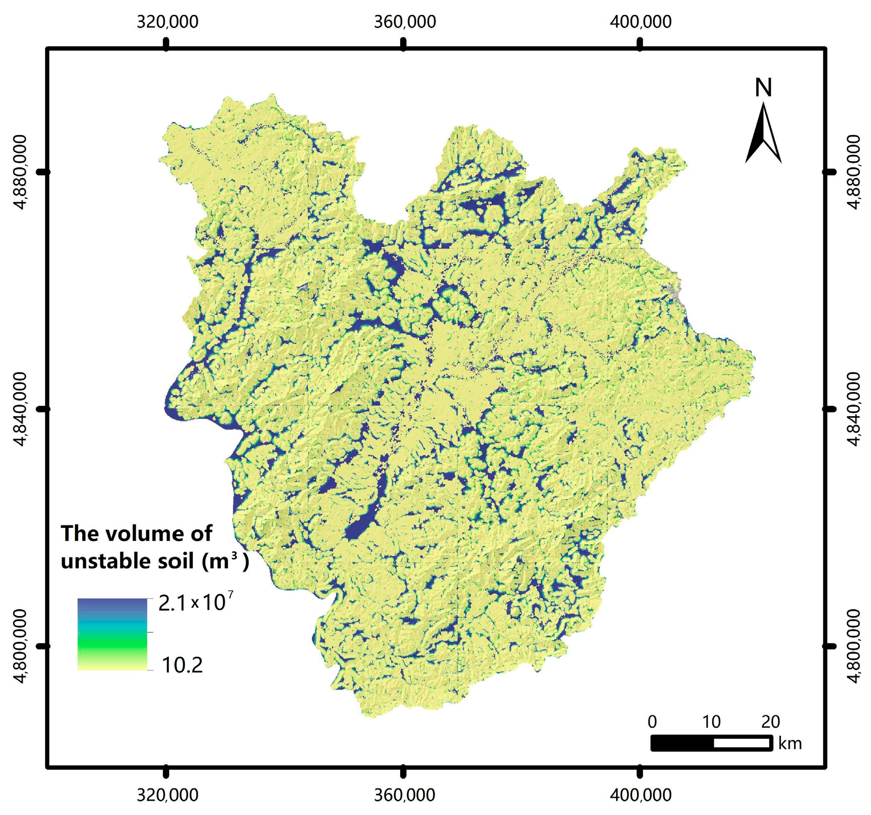Firstly, precipitation is coupled with slope soil, which makes the soil on the slope unstable; secondly, debris flow is formed by the coupling of runoff and unstable soil [6]. Based on the mechanism of debris flow formation, this forecast method established a coupling relation between the rainfall and unstable soil of the underground surface. The density of the mixture reaching a certain threshold is a necessary condition for the debris flow to form. Therefore, the density of the debris flow is introduced as an evaluation index to determine the susceptibility of debris flow occurrence. To calculate the density of the mixture, the first phase of the forecast method based on the rainfall-unstable soil coupling mechanism (R-USCM) needs to determine the volume of unstable soil, and the second phase needs to determine the volume of the runoff.

An accurate calculation of the amount of unstable soil failure is crucial in the first phase of the forecast method based on the R-USCM. It is also an indispensable factor for a number of hazard assessments, sediment budgets, and initial conditions for landslide run-out models. The 2D model has been widely used to analyze slope stability. However, a traditional 2D slope stability analysis (SSA) cannot consider the direction of the slip surfaces, and failure bodies are forced to move in the presupposed direction. Furthermore, the traditional 2D model assumes that the sliding surface is parallel to the slope, which may not be completely consistent with the actual slope instability [15]. To estimate the sum of the volumes of unstable soil, detailed data about the soil thickness are essential, which is hard to acquire for a large regional scale. Thus, it is still a huge challenge to obtain the relevant complete data essential to use a traditional 2D model to calculate the sum of the volumes of the unstable soil for forecasting debris flows.

Therefore, the 3D deterministic model Scoops3D is adopted in this paper to evaluate and predict the stability of unstable soil. The model uses the circular arc method to search for sliding surfaces with different curvatures in the study area in 3D space and uses the limit equilibrium method to analyze the stability of each grid based on the digital elevation model (DEM) SSA data. This solves the problem where the sliding surface is parallel to the slope surface, which is inconsistent with the actual situation. Furthermore, Scoops3D computes the volume of each column in the potential failure mass and adds it to the total. It also does not ignore the columns along the margin of the potential failure mass, which may be only partly contained within the scopes of the sphere. Thus, the volume of the unstable soil is calculated more accurately. In addition, the 3D SSA usually provides more stable results than the one-dimensional (1D) and 2D methods [16,17,18], and it is demonstrated that the Scoops3D model has the potential to overcome the problem of over-prediction. According to the above, using the Scoops3D model to determine the volume of unstable soil can improve the accuracy of the forecast method based on the R-USCM.

In this paper, the forecast method based on the R-USCM is used to predict debris flows in Jiaohe County, Jilin Province. The serious debris flow disaster attributed to strong rainfall in Jiaohe County on 20 July 2017, was taken as the research case. The Scoops3D model and traditional 2D method are used to analyze the slope stability and calculate the volume of unstable soil. The soil conservation service (SCS) curve number (CN) method is used to calculate the volume of the runoff. The Scoops3D model combined with the SCS-CN method is called the S-CN forecast method, and the traditional 2D model combined with the SCS-CN method is called the T-CN forecast method. In order to test the forecasting ability of the two methods, the forecasting results of the two methods were compared with the debris flow distribution map for Jiaohe County and tested by the receiver operating characteristic (ROC) curve method.

2. Forecast Method of Debris Flow Based on the Rainfall-Unstable Soil Coupling Mechanism

2.1. Forecast Theory

Soil is unsaturated before persistent or heavy rainfall infiltration, being in a relatively stable state. However, the gradual increase in the soil moisture caused by rainfall infiltration will reduce the matrix suction and apparent cohesion of the soil, thereby reducing the shear strength of the soil. Therefore, in the case of short-term heavy or continuous rainfall, runoff and unstable soil can cause debris flows. According to the R-USCM, the process of debris flow formation can be simplified into two phases: The first phase is the soil on the slope becomes unstable due to rainfall, which provides a sufficient source basis for the generation of debris flows; the second phase is that the unstable soil will form a debris flow when it encounters runoff.

However, so far the processes of the debris flows formation are too complex to be simulated by numerical and physical models. Debris flow can be considered to consist of water and sediment. The density of the sediment in the debris flow reaching a certain threshold is a necessary condition for debris flow to form. Therefore, the density of the debris flow is introduced as an evaluation index to determine the susceptibility of debris flow occurrence. However, the density of debris flow changes continuously during the process of formation. Therefore, the complex dynamic rainfall-unstable soil coupling process is expressed quantitatively with the static coupling results. Specifically, this means using runoff and unstable soil caused by rainfall to calculate the density of the mixture. The susceptibility of debris flow occurrence has been judged by the density we have calculated.

$$\rho =\frac{{\rho }_r{\upsilon }_r+{\gamma }_{us}{\upsilon }_{us}/g}{{\upsilon }_r+{\upsilon }_{us}}$$

(1)

where $\rho$ is the density of the debris flow, ${\rho }_r$ is the density of the runoff, and ${\gamma }_{us}$ is the unit weight of the unstable soil. $g$ is the acceleration of gravity, ${\upsilon }_r$ is the volume of the runoff, and ${\upsilon }_{us}$ is the volume of the unstable soil which can provide the material source basis for the debris flow. Therefore, according to Equation (1), the accurate calculation of ${\upsilon }_r$ and ${\upsilon }_{us}$ is an important part of evaluating the accuracy of the forecast method based on the R-USCM.

According to the previous research [19], the density of the standard debris flow fluctuates between 1.1 × 10³ and 2.3 × 10³ kg/m³. We divided the density of the mixture into five reference intervals, as shown in

Table 1. The susceptibility of debris flow occurrence based on the water-soil mixture density.

The Density of Debris Flows	Class	Susceptibility of Debris Flow	Color of Warning
$\rho$ < 1.2	1	Very low	Blue
1.2 < $\rho$ < 1.5	2	Low	Green
1.5 < $\rho$ < 1.8	3	Moderate	Yellow
1.8 < $\rho$ < 2.0	4	High	Orange
2.0 < $\rho$ < 2.3	5	Very high	Red

. They are used as a criteria for evaluating the susceptibility of debris flow occurrence from low to high. Based on these density intervals, five levels of debris flow warnings were determined (Table 1). Figure 1 shows the flowchart of the debris flow prediction method based on the R-USCM.

2.2. The Volume of Unstable Soil Calculated by the Scoops3D Model

The 3D slope stability assessment has not been widely used due to its intricacy, its computational requirements, and the lack of relevant data. The majority of methods use 1D (infinite slope model on a raster cell-by-cell basis) [20,21] or 2D (based on a series of obtained by DEM) [22] models to evaluate the slope stability. Some scholars have noted that 1D and 2D models are receivable in SSA; not only are their calculations easier, but they also provide more cautious results than 3D models [23]. However, they may not simulate the practical mechanism of the motion process of unstable soil [15]. Compared to other models, the Scoops3D model has the advantage of considering the terrain described by DEM to identify various potential sliding bodies in the whole region, not just for a single landslide on the pre-defined hill-slope. If materials have no sharp contrast or discontinuity, the failure is usually curved. According to this feature, Scoops3D uses the potential failure or slip surface made by parts of a sphere and presumes a rotational slip. Through a 3D analysis, the Scoops3D model provides direct estimates of the potential failure volume. The result of the calculation is more accurate than that of traditional models. This can also improve the accuracy of the forecast method based on the R-USCM.

Scoops3D analyzes the stability of each grid based on the DEM data. First, the sliding surface is determined in order to calculate the weight of the potential slide block, and then the stability of the object is calculated by the 3D limit equilibrium method. In the process of calculation, a 3D retrieval region is established based on the grid of the DEM. A mass of search points are identified in the region. Each search point is taken as the center of the ball in turn, and the search is expanded according to a certain radius. The grid element that is finally delineated by the sphere is the sliding block [24]. Since the bottom of each grid element is part of the sphere, the surface is approximately treated as a plane with an angle of $\epsilon$ to the horizontal plane [24].

Scoops3D calculated the shear strength through the linear Coulomb-Terzaghi instability criterion [25].

$$s=c+\left({\sigma }_n^{}-u\right)\tan \varphi$$

(2)

where $c$ and $\varphi$ are the apparent cohesive force and angle of internal friction of the soil, respectively. ${\sigma }_n^{}$ is the normal stress of the sliding block, and $u$ is the pore water pressure acting on the shear surface.

Limit equilibrium models define $F$ as the ratio of the shear resistance (s) to the shear stress ($\tau$). $F$ < 1 shows the slope is in an unstable state in theory.

We choose the 3D expansion method of Bishop's simplified model for the limit equilibrium model because it provides a simple and effective solution for a large number of practical problems [26]. In the Scoops3D model, the main force from the downward sliding of soil comes from gravity on the slider, in addition to the action of a seismic load (K_eqW). K_eq is the horizontal acceleration coefficient, and the following formulas are used to calculate the safety factor using the 3D simplified Bishop method [24].

$$F_{3D}=\frac{\Sigma R_{i,j}\left[c_{i,j}{A}_{h_{i,j}}+\left(W_{i,j}-u_{i,j}{A}_{h_{i,j}}\right)\tan {\varphi }_{i,j}\right]/m_{{\alpha }_{i,j}}}{\Sigma W_{i,j}\left(R_{i,j}\sin {\alpha }_{i,j}+k_{eq}{e}_{i,j}\right)}$$

(3)

$$m_{{\alpha }_{i,j}}=\cos {\epsilon }_{i,j}+\left(\sin {\alpha }_{i,j}\tan {\varphi }_{i,j}\right)/F_{s3D}$$

(4)

The calculation of unstable soil volume is a key step in SSA, Scoops3D computes the volume ($V_c$) of each column which may be unstable and adds it to the total. Some of the columns distributed on the margin of potential failure surfaces may only be partially contained within spherical boundaries. When two or three corners of columns are contained within the spherical trial surface, Scoops3D can recognize them and take the incomplete volume of the columns into account, rather than full columns that other approaches use exclusively. Therefore, Scoops3D can accurately give the estimates of the volume of the unstable soil [24].

The volume of each column (partial or full), which is above the trial surface, can be approximately calculated by the following equation:

$$V_c=\left(1/6\right)\Delta x\left(S_0+4S_1+S_2\right)$$

(5)

where $\Delta x$ represents the DEM mesh spacing, $S_0$ and $S_2$ are the superficial areas of the two parallel sides of the column, and $S_1$ is the superficial area of a vertical cross section through the middle of the column [24].

For full column, its area calculation becomes the calculation of the quadrilateral area, and its volume calculation becomes the calculation of the cube volume. For those partial columns with two nodes, its area calculation becomes the calculation of the triangular area, and its volume calculation becomes the calculation of the pyramid volume. For those partial columns with three nodes, the shape of one side is roughly a quadrilateral, whereas the other side is a triangle [24].

2.3. Runoff Volume

The runoff depth plays an important role in water space redistribution. To estimate the runoff depth and thus obtain the total volume of the runoff, the SCS-CN method is applied [27]. The runoff depth is used to assess the potential water supply during runoff. Its most recent calculated equation was published by the Natural Resource Conservation Service (NRCS) in 2004:

$$Q=\frac{{\left(P-I_a\right)}^2}{\left(P-I_a\right)+R}$$

(6)

where Q is the runoff depth (mm), P is rainfall (mm), R is the potential maximum retention after the runoff begins (mm), and $I_a$ is an initial abstraction (mm) that includes all losses before the beginning of runoff, evaporation, infiltration, and water interception by plants. It is defined as:

$$I_a=\lambda R$$

(7)

According to the reference of NRCS, the value of $\lambda$ in this study is 0.2 [28]. Equation (6) can therefore be expressed as:

$$Q=\frac{{\left(P-0.2R\right)}^2}{\left(P+0.8R\right)}$$

(8)

R can be calculated by the following equation through the relationship between R and CN:

$$R=\frac{25,400}{CN}-254$$

(9)

CN provided by the Soil Conservation Service is an important indicator of the runoff depth. CN ranges from 0 to 100, representing the runoff response to a given rainfall event. The higher the value of CN is, the more rainfall is converted to surface runoff [27,29]. The values of CN are determined by the effect of runoff on soil and land cover. Therefore, the value of CN for each pixel in the study area can be estimated according to the soil-texture and land cover maps. In other words, the antecedent runoff conditions (ARCs) determine the selection of the CN value. ARC level is determined by the actual pre-rainfall of the debris flows. The ARC can be divided into three levels: ARC I represents dry, ARC III represents wet, and ARC II accounts for the antecedent runoff condition between dry and wet [27]. After determining the ARC level, the corresponding value of CN can be obtained from the data provided by NRCS.

Then, the sum of the volumes of runoff ${\upsilon }_r$ which resulted from the rainfall can be calculated using the following formula:

$$Su{m}_{v_r}={\displaystyle \sum _{i=1}^N{S}_i}\times Q_i$$

(10)

where $Su{m}_{v_r}$ is the total volume of the runoff, $Q_i$ is the runoff depth of each grid cell, $S_i$ is the area of each grid cell, and $N$ is the total number of grid cells.

3. Debris Flow Prediction and Test in the Study Area

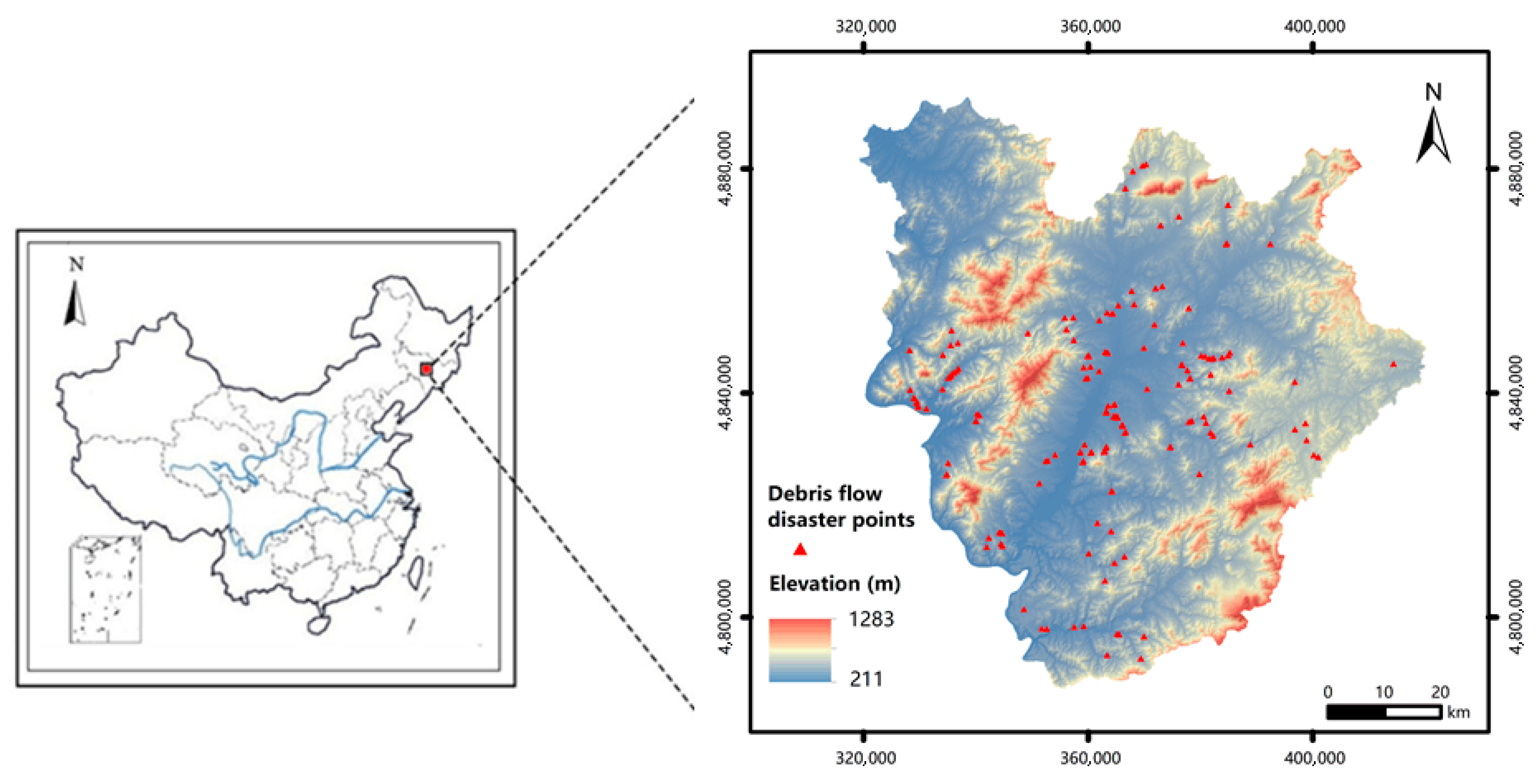
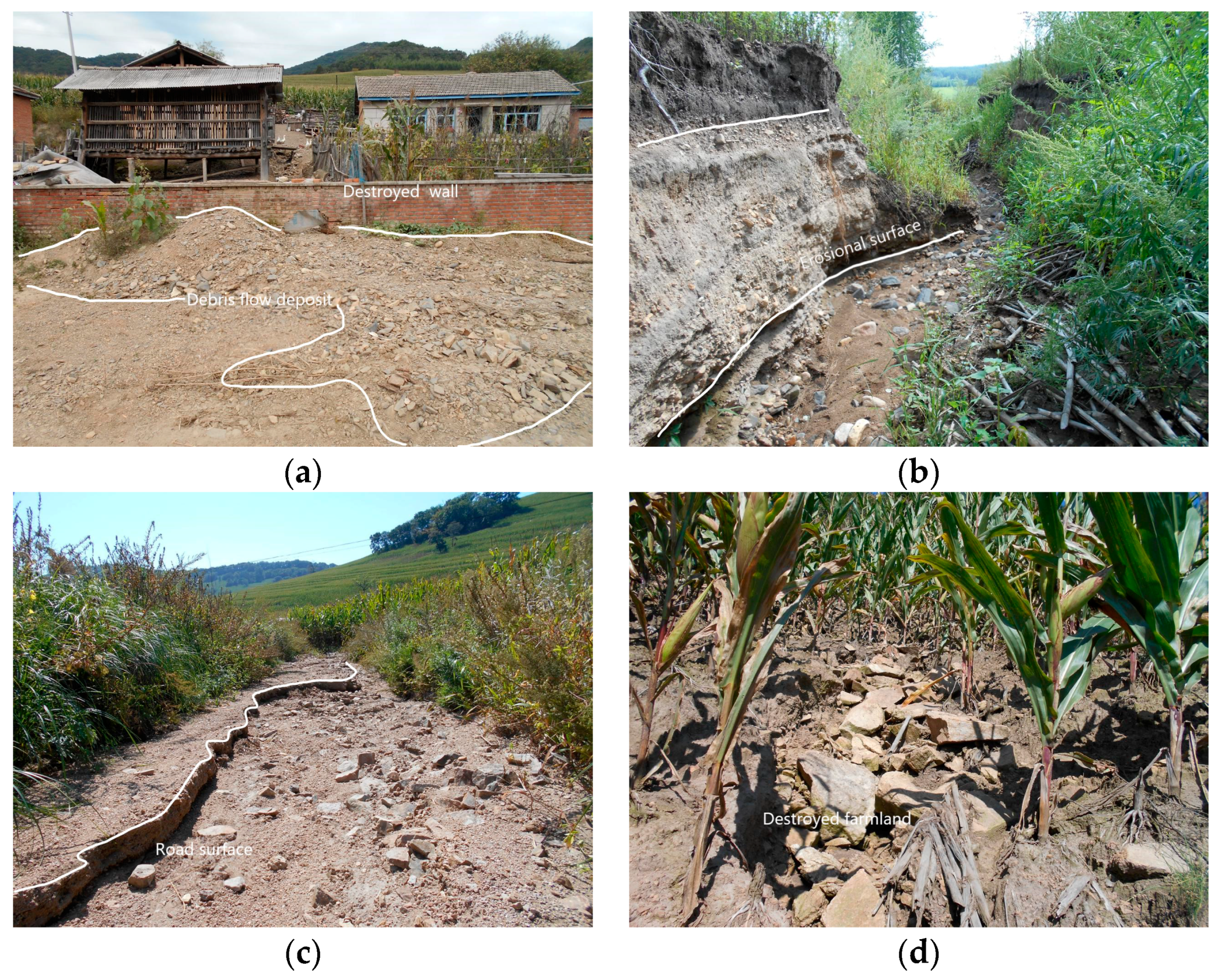
Jiaohe County is prone to geological disasters and is one of the regions with the most severe geological catastrophes in Jilin Province. Because debris flow has several divisions within one zone, more hazardous geological disasters occur [30]. In the past several years, debris flows frequently occurred in the area due to strong rainfall, which has caused a great loss of local residents’ lives and properties. Until 2017, a geological survey of Jilin province at a 1:50,000 scale found 162 debris flow disaster locations (Figure 2), with 23,231 square kilometers of crops affected, 1766 houses damaged, more than 59 km of roads damaged, 91 bridges and 7 culverts damaged, and 79 landslides and other geological disasters produced. The direct economic loss was approximately 202.62 million yuan (Figure 3). On 20 July 2017, Jiaohe County suffered strong rainfall which caused serious debris flow disasters. The debris flow disasters and rainfall event was used here as a study case. The forecast method based on R-USCM was developed for Jiaohe County, including the S-CN and T-CN forecast methods. The forecast results were compared with the debris flow hazard points discovered by the 2017 geological survey of Jilin province at a 1:50,000 scale, and then a preliminary assessment of the accuracy was made.

3.1. Calculate the Volume of Failure Soil Mass Caused by Rainfall in Jiaohe County

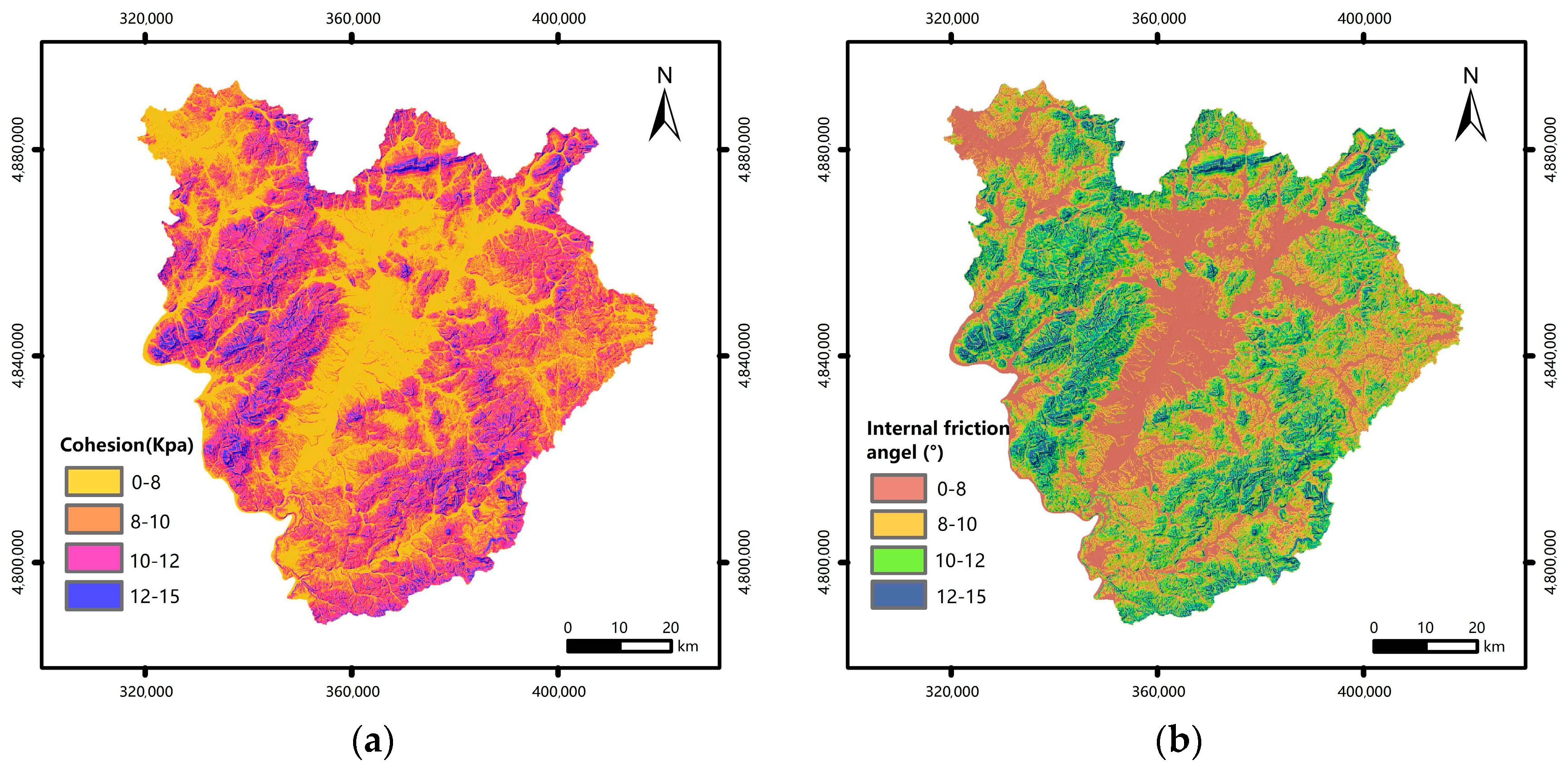
Scoops3D predicted the soil stability and calculated the volume of failure soil based on the DEM and soil mechanical parameters in Jiaohe County. The DEM of Jiaohe County with a spatial resolution of 7 × 7 m was obtained from Google Earth by using the software of 91 graphic assistant (v16.9.9.2, Beijing Qianfanyunlian technology co. LTD, Beijing, China, 2018) (Figure 4). The mechanical parameters of the soil include soil cohesion $c$, internal friction angle of soil $\varphi$ and soil unit weight $\gamma$. 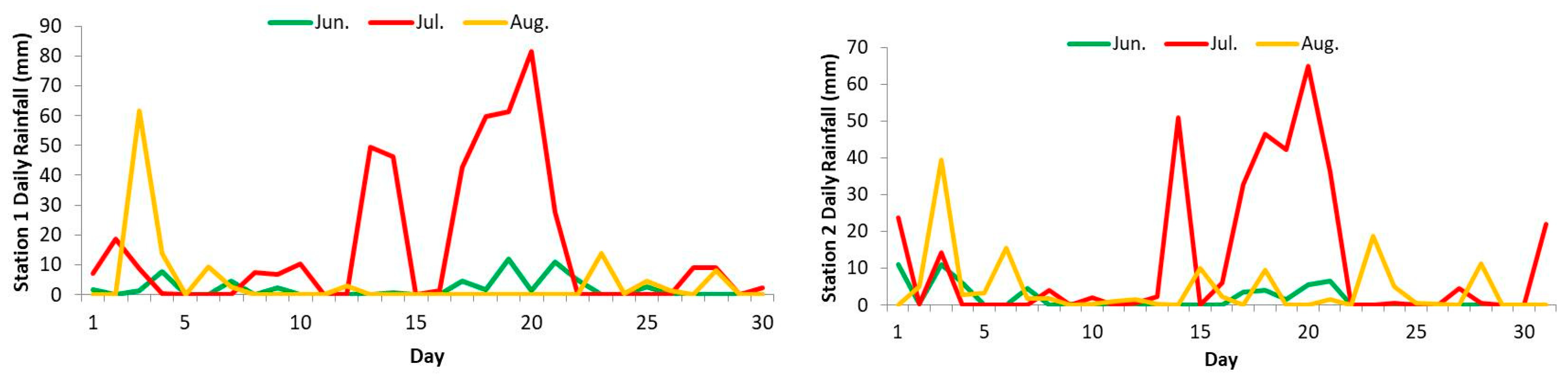Lithology data were extracted from the geological map of Jilin Province at a 1:50,000 scale, and the mechanical parameters were derived from the rock mechanics manual. According to the rainfall data from the two observation stations in Jiaohe County (Figure 5), the debris flows occurred on 20 July and continuous rainfall preceded the day that debris flow occurred. Concentrated and continuous heavy rainfall will significantly increase the water content and reduce the strength of the soil, and the stability of the slope will decrease. Therefore, the mechanical parameters of soil under wetting conditions with 30% gravimetric water content were selected as the input parameters of debris flow forecast methods (Figure 6). According to the rock mechanics manual, the unit weight of the soil is 1.75 × 10⁴ kN/m³ when the soil is under wetting conditions with 30% gravimetric water content. The Scoops3D model can directly generate the volume of unstable soil according to the above parameters set (Figure 7).

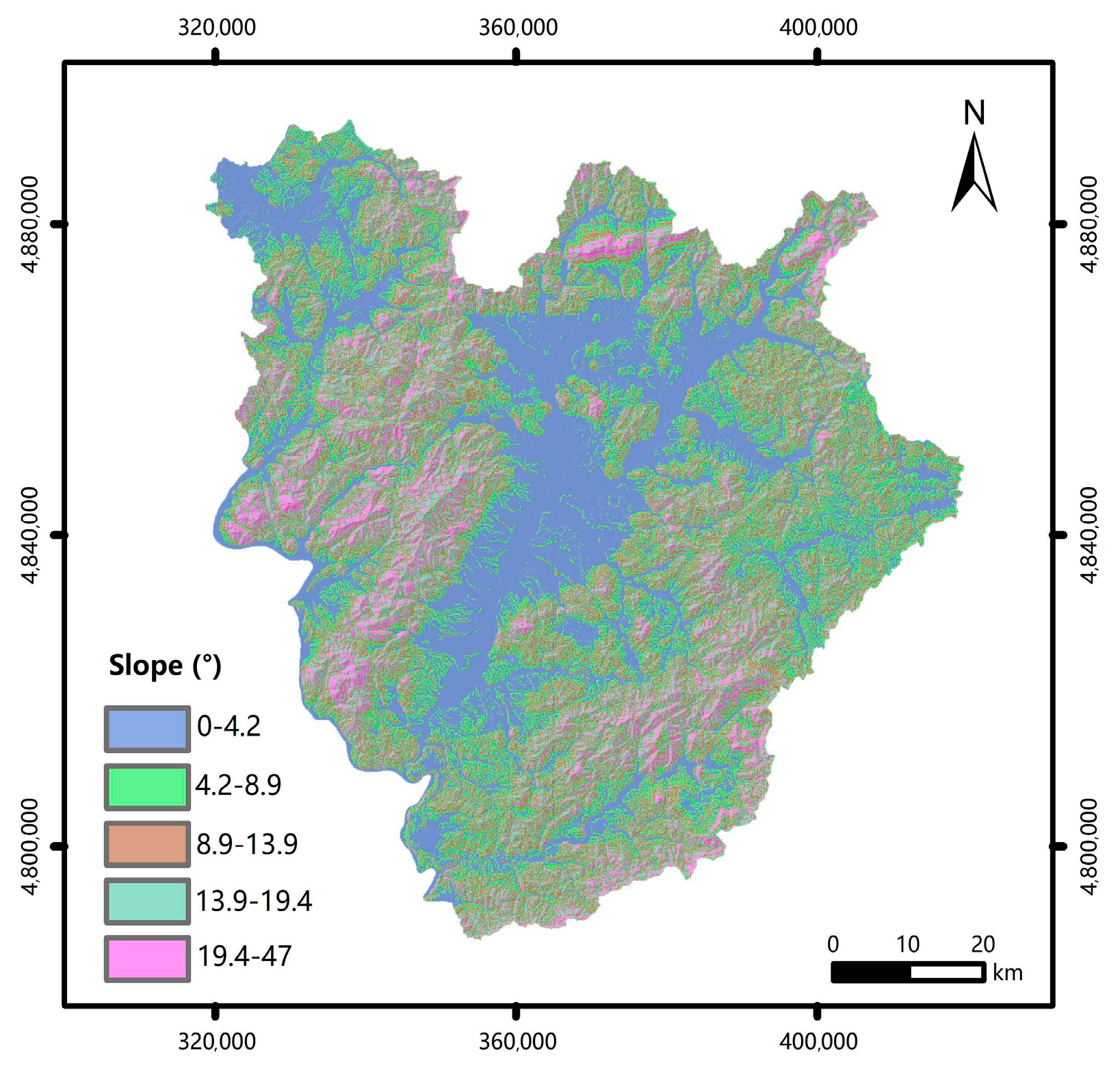
To calculate the volume of the unstable soil using a traditional 2D method, the thickness of the unstable soil should first be determined. In the current research, the soil thickness was obtained by using the relation between the slope and soil thickness proposed by Veit et al [31]. It can be approximated that there is a linear relationship between soil depth and slope angle [23]. The slope was directly extracted from the DEM (Figure 8). In this way, the soil depth of an any pixel (y) can be calculated by the function y = −0.0486x + 3.5. After determining the total thickness of the soil, several layers were subdivided, and the safety factors of each layer were calculated. More details about soil thickness are provided in

Table 2. Soil thickness in Jiaohe County, Jilin Province.

Class	Thickness (m)	Relative Area (%)	Thickness of Subdivided Soil Layers
			1	2	3	4	5	6	7
I	3.25–3.30	7.10%	0.1	0.2	0.3	0.4	0.5	0.75	0.95
II	3.30–3.35	39.06%	0.1	0.2	0.3	0.4	0.5	0.75	1.00
III	3.35–3.40	24.59%	0.1	0.2	0.3	0.4	0.5	0.75	1.05
IV	3.40–3.45	29.25%	0.1	0.2	0.3	0.4	0.6	0.75	1.10

. The mechanical parameters of the soil required for the traditional 2D method are the same data used in the Scoops3D model. It is essential to resample these data to ensure the grid cells are of the same size as the DEM. Then, the sum of the volumes of the unstable soil in the study area was calculated by Equation (11) and is shown in Figure 9.

$$Su{m}_{v_s}={\displaystyle \sum _{i=1}^{N_{}}{S}_i}\times D_i$$

(11)

where $Su{m}_{v_s}$ is the sum of the volumes of the unstable soil, $D_i$ is the unstable soil thickness of each grid cell, $S_i$ is the grid cell area, and $N$ is the sum of the numbers of the unstable grid cells.

3.2. Calculate the Runoff Volume in Jiaohe County

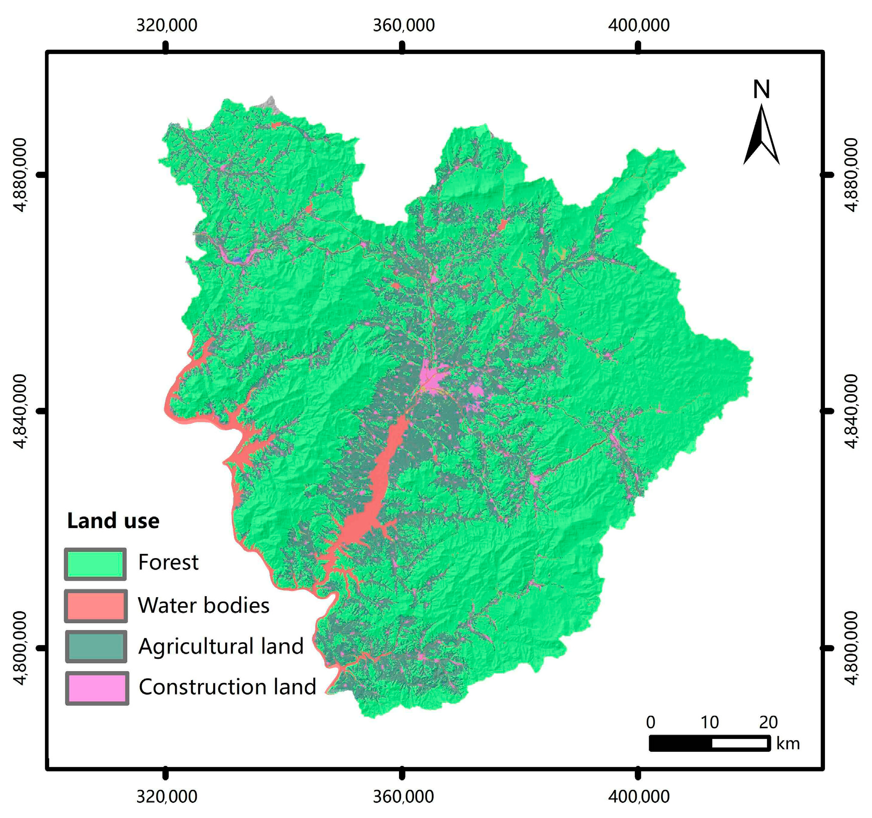
The volume of runoff was calculated by the SCS-CN method, which required the CN values and rainfall data. The CN values are determined by land use. Land use in Jiaohe was determined from a geological map of Jilin province at a 1:50,000 scale, including agriculture land, forest, irrigation canals and ditches, and other scarce vegetation (Figure 10). The CN values are provided in

Table 3. Curve number (CN) values reflecting antecedent runoff condition III (ARC III).

Land Use	CN
Agriculture land	95
Forest	89
Irrigation canals and ditches	88
Other scarce vegetation	97

[27].

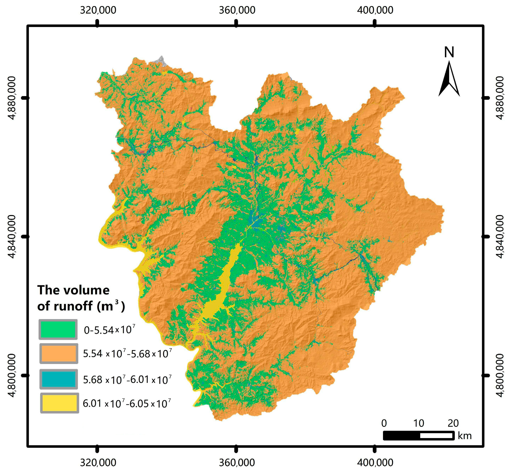
There are two weather stations in Jiaohe County. Based on the rainfall data from weather stations, the annual precipitation is unevenly distributed, primarily concentrated from June to August. The daily rainfall curves from July to August (2017) are shown in Figure 5. According to different types of data sources, such as historical records, field surveys, and interviews with local residents, it can be determined that the large-scale debris flow caused by rainfall occurred on 20 July 2017. Daily rainfall around the north and south of the weather stations reached 81.6 and 65 mm, respectively. Therefore, debris flow in Jiaohe is predicted using the forecast method based on the R-USCM under the same rainfall conditions as 20 July 2017.

Combined with the rainfall data and CN values in Jiaohe County, the total volume of runoff can be obtained according to Equation (10) (Figure 11).

3.3. Calculate the Density of the Water-Soil Mixture in Jiaohe County

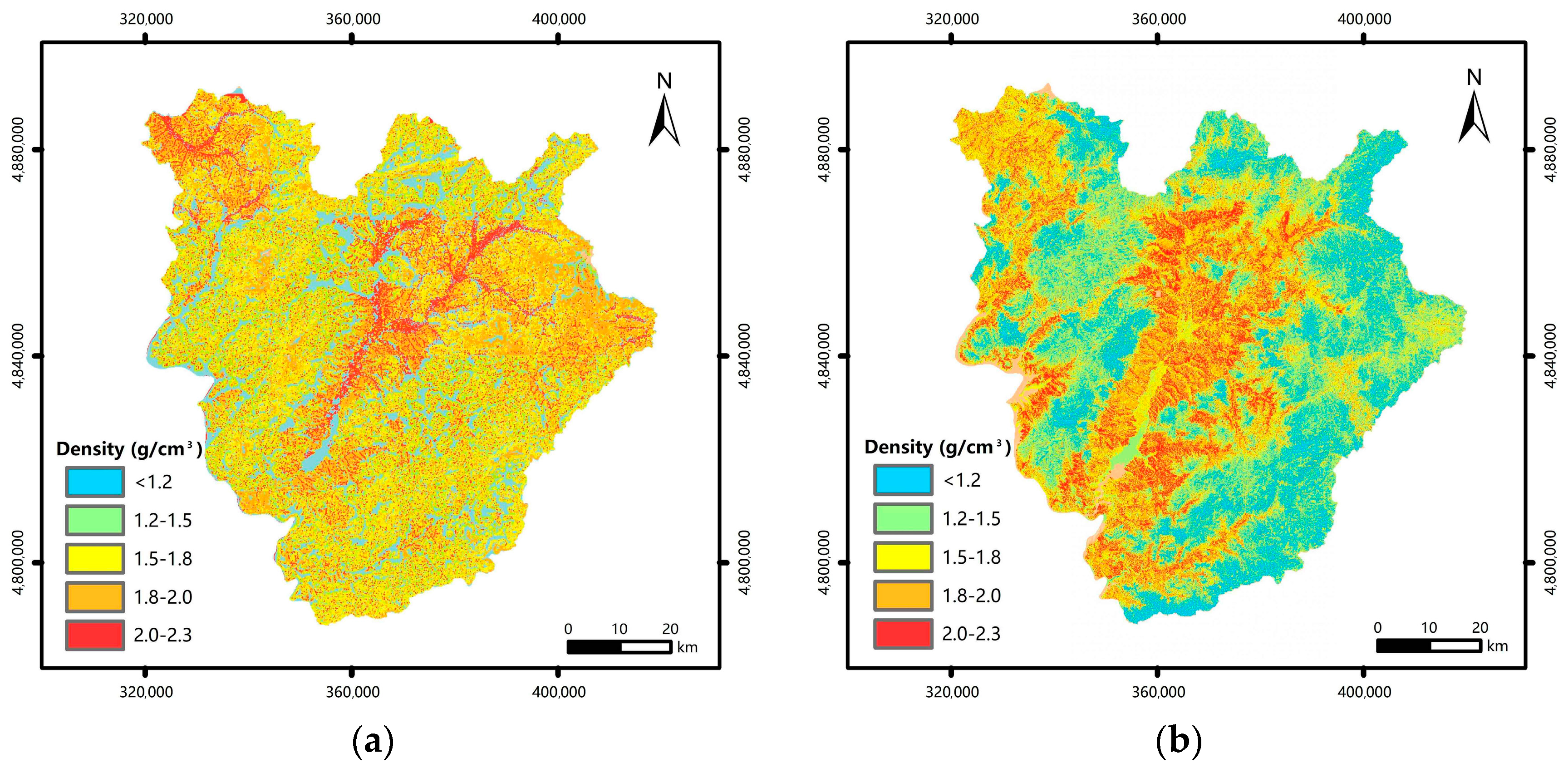
According to Equation (1), the maps of the water-soil mixture density calculated by the S-CN method and T-CN method are shown in Figure 12.

4. Forecast Results and Discussion

In order to forecast the areas susceptible to debris flows, the density of the water-soil mixture and the corresponding susceptibility must be referenced (Table 1). Therefore, early alerts for areas susceptible to debris flows can be derived from the maps of forecast results (Figure 13). This is important for providing an effective theoretical basis for geological disaster prevention, control planning and risk management. As a result, loss of property and life can be reduced when debris flow occurs.

We analyzed the predicted results provided by the S-CN and T-CN forecast methods under the same rainfall conditions as 20 July 2017. This makes it possible for us to compare the prediction results with the field survey debris flow disaster points and evaluate the prediction ability macroscopically based on the R-USCM. In general, according to the predicted results by the S-CN and T-CN forecast methods, there are 22,391 and 33,024 km² in the very high and high susceptibility areas which accounted for 34.39% and 50.72% of the total study area, respectively. In addition, very low and low susceptibility areas only accounted for 32.58% and 27.25% of the total study area. It is shown that the study area belongs to the areas susceptible to debris flows, which is consistent with the actual investigation.

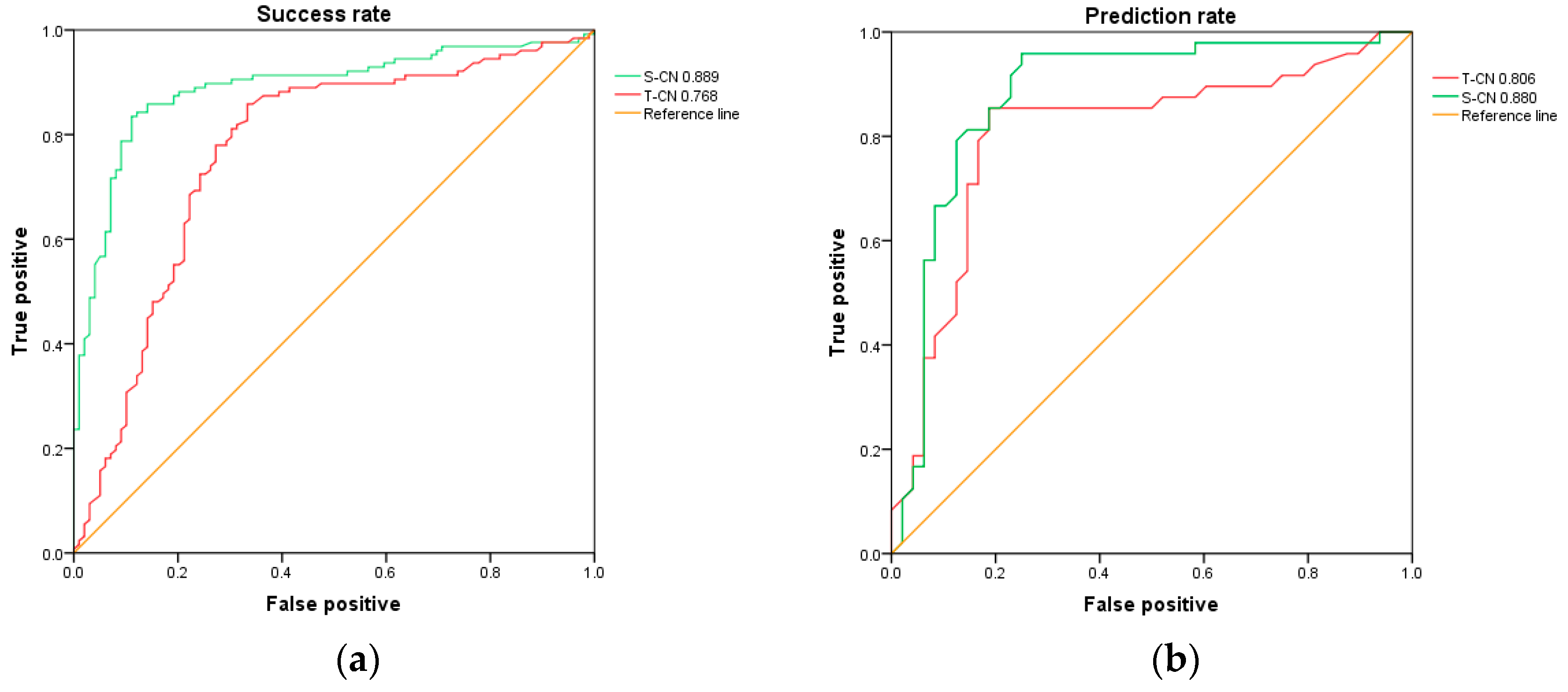
In this paper, the ROC curve method which is an effective tool to determine the quality of forecast methods, is also used to evaluate the prediction results of the two methods. The area under the ROC curve (AUC) represents the accuracy of a reliable probabilistic model for forecasting the occurrence or non-occurrence of debris flows. The reference line serves as the standard for judging the degree of model fitting. When AUC is greater than 0.5, the model fits well, and when AUC is less than 0.5, the model fits randomly. The most common method is to use the success rate and prediction rate curves to verify the model. The success rate curve is used to determine how well the maps of forecasting results have classified the areas of existing debris flows. The prediction rate curve shows how well the model and predictor variables predict debris flows. Both success and prediction rate curves are shown in Figure 14. The AUC values for the S-CN model and the T-CN model are 0.889 (88.9%) and 0.768 (76.8%), respectively. The prediction rate curves show that the AUC values for the S-CN model and T-CN model are 0.880 (88.0%) and 0.806 (80.6%), respectively, demonstrating that the S-CN model and T-CN model have a good performance for debris flow forecasting.

Furthermore, under the same conditions of runoff, it can be seen that the prediction accuracy can be improved by using the Scoops3D model to determine the volume of the unstable soil mass. The Scoops3D model uses a circular arc search sliding surface method to determine the unstable slope surface, overcoming the shortcomings of the 2D method, which assumes that the failure surface is parallel to the slope surface. Scoops3D conducts SSA based on DEM of the study area. Due to the fact that the topographic features are an important factor affecting the slope stability, it can be preliminarily confirmed that the forecast results of the Scoops3D model have a high fit with the actual distribution of the unstable slopes. Beyond that, the Scoops3D computes the volume of each column in the potential failure mass and adds it to the total. This includes partial columns in the volume computation if two or three corners of the column at the ground surface are contained within the spherical trial surface, rather than full columns that other approaches use, especially when the potential failure mass includes only a small number of full columns. The Scoops3D model can calculate the volume of unstable soil more accurately.

According to the prediction rate curve, the prediction rate of the S-CN model is higher than that of the T-CN model. As seen from Figure 13, although the susceptibility area predicted by the T-CN method is larger, The Scoops3D model usually provides more stable results than the 2D methods in SSA. This is because in the analysis stage of Scoops3D model, although most safety factors of the searched unstable sliding surface are low, the stability of the partial region is improved due to the influence of local micro-geomorphology. Therefore, it is shown that the S-CN method has the ability to overcome the over-prediction problems in debris flow forecasting.

Figure 13 shows that the distribution map of debris flow obtained by the S-CN method is more realistic than that by the T-CN method in terms of the distribution characteristics of debris flow. It can be seen from Figure 13a that the debris flow tends to occur in small individual watershed areas instead of scattered points. The reason for this distinction is that in the analysis of slope stability, each soil column has its individual Fs value, which is separate from other cells in the traditional 2D method. There are some scattered unstable cells even in places far from the sliding sites. However, in the Scoops3D model, slip surfaces tend to occur in a single block, and a hypothesis must be made in order to aggregate unstable pixels together and define landslide blocks, which makes them readily observable. It also makes the result more reasonable.

According to the predicted results by the S-CN and T-CN forecast methods, there are 135 and 116 debris flow disaster locations in the very high and high susceptibility areas which accounts for 83.33% and 71.60% of the total debris flow disaster locations, respectively. No trace of debris flows has been found in partial very high and high susceptibility areas, which may be due to the occurrences of small-scale debris flows in these locations in the past. These traces may be destroyed or covered by plants. Field investigations can only determine the recent development of debris flows. In order to further validate, it is necessary to conduct detailed surveys on the spatial and temporal scales of the study area in the later stage. There are 15 and 24 debris flow disaster locations in the very low and low susceptibility areas which accounts for 9.26% and 14.81% of the total debris flow disaster locations, respectively. This is probably because in the actual conditions, climatic conditions, ground fissures, earthquakes, and other effects will lead to the instability of the slope. However, the current forecast methods cannot incorporate all factors into the SSA. Slope instability caused by factors not included in the SSA cannot be predicted. Therefore, it will affect the accuracy of the debris flow forecast method based on R-USCM. Another influence factor is due to the limited number of rainfall observation stations and the finiteness of the method to collect rainfall data, which makes it very difficult to accurately obtain the daily accumulated rainfall in each location of Jiaohe County. Based on the data of two rainfall observation stations, all of Jiaohe County is divided into two parts. In each part of Jiaohe County, different locations may have different amounts of rainfall over the same time period, so it is not reasonable to use the rainfall station data to represent the rainfall values for the entire region. Therefore, calculating the runoff by using the SCS-CN method in this paper may lead to errors. Further research should use a reasonable method for determining the accurate rainfall values of each location.

Finally, we emphasize that the use of the 3D method to find slip surfaces based on a high-precision DEM is usually time-consuming. The Scoops3D model cannot run in a geographic information system (GIS) environment nor can it realize parallel computing on multicore machines. Allowing very large areas to be simulated in a short time is the next step that requires improvement.

5. Conclusions

In the current study, a debris flow forecasting method based on the R-USCM is proposed. The key to the R-USCM is calculating the volume of unstable soil and the volume of runoff. The Scoops3D model was applied in calculating the volume of the unstable soil because it can analyze the stability of the slope according to the actual situation and calculate the volume of the unstable soil more accurately. The SCS-CN method was also applied in calculating the volume of runoff. The accuracy and applicability of the S-CN were proved in the case study in Jiaohe County. The results are compared with those of the T-CN method. Through the detailed analysis of the forecast results, the following conclusions can be made:

(1) The prediction model of the debris flow based on the R-USCM is due to the formation mechanism of debris flow. The coupling relations between the rainfall and unstable soil from the slope is established. As long as the unstable soil and rainfall information are obtained at the regional scale, a debris flow forecasting method can be used to predict the susceptibility of the debris flows at the regional scale. Thus, the debris flow forecasting method based on the R-USCM has strong applicability.

(2) The use of this S-CN method based on the R-USCM can successfully forecast debris flows at the regional scale. According to the results from the ROC curve, the method had a higher success and prediction rate than the T-CN method. It can be determined that the accuracy of calculating the volume of unstable soil when runoff conditions are the same can also influence the forecasting results. Therefore, compared with the traditional 2D model, the Scoops3D model has a higher precision and better adaptability in analyzing the slope stability and calculating the volume of the unstable soil.

(3) The distribution characteristics of debris flow are largely determined by the distribution characteristics of unstable soil. It can be seen from Figure 13 that the S-CN method provides a more realistic result than the T-CN method. The debris flow tends to occur in small individual watershed areas instead of scattered points. The main reason is that the Scoops3D identifies the unstable sliding surface instead of some scattered unstable cells. Slip surfaces also tend to occur in individual blocks. Therefore, the risk map generated by the S-CN method is better applied in debris flow control and early warning.

(4) The results show that the T-CN method has the problem of excessive prediction of debris flow. The prediction of a dangerous area is too large to properly measure for early warning. It is certain that the over-prediction problems of the traditional 2D method of calculating the unstable soil can also influence the results. Because of the use of the Scoops3D models, the S-CN method has the ability to overcome the over-prediction problems in debris flow forecasting to provide a reliable basis for geological disaster prevention, control planning and risk management.

In conclusion, it is convincing that the Scoops3D model combined with the SCS-CN method is a practical tool for a 3D, spatially-distributed assessment and forecast of debris flow base on the R-USCM. At present, this method can only predict the debris flow susceptibility zone and cannot realize the prediction of the size of the debris flow trigger area. Further development of this work should focus on drawing orthophotographic maps of the research area to identify the actual scale and hazard scope of each debris flow. This reforming will help to evaluate the size of the debris flow triggering area in detail, thus allowing case-by-case comparisons between the model predictions and field reality. In addition, future research should also use a more reasonable method to determine the rainfall in each location of Jiaohe County and consider more comprehensive factors in SSA. More accurate forecasting results can be obtained.