Article

ELM-Based AFL–SLFN Modeling and Multiscale Model-Modification Strategy for Online Prediction

School of Automation, Central South University, Changsha 410083, China
*
Author to whom correspondence should be addressed.
Processes 2019, 7(12), 893; https://doi.org/10.3390/pr7120893
Submission received: 21 October 2019 / Revised: 21 November 2019 / Accepted: 26 November 2019 / Published: 1 December 2019

Abstract

:
Online prediction of key parameters (e.g., process indices) is essential in many industrial processes because online measurement is not available. Data-based modeling is widely used for parameter prediction. However, model mismatch usually occurs owing to the variation of the feed properties, which changes the process dynamics. The current neural network online prediction models usually use fixed activation functions, and it is not easy to perform dynamic modification. Therefore, a few methods are proposed here. Firstly, an extreme learning machine (ELM)-based single-layer feedforward neural network with activation-function learning (AFL–SLFN) is proposed. The activation functions of the ELM are adjusted to enhance the ELM network structure and accuracy. Then, a hybrid model with adaptive weights is established by using the AFL–SLFN as a sub-model, which improves the prediction accuracy. To track the process dynamics and maintain the generalization ability of the model, a multiscale model-modification strategy is proposed. Here, small-, medium-, and large-scale modification is performed in accordance with the degree and the causes of the decrease in model accuracy. In the small-scale modification, an improved just-in-time local modeling method is used to update the parameters of the hybrid model. In the medium-scale modification, an improved elementary effect (EE)-based Morris pruning method is proposed for optimizing the sub-model structure. Remodeling is adopted in the large-scale modification. Finally, a simulation using industrial process data for tailings grade prediction in a flotation process reveals that the proposed method has better performance than some state-of-the-art methods. The proposed method can achieve rapid online training and allows optimization of the model parameters and structure for improving the model accuracy.

1. Introduction

Data-based modeling is becoming important in the field of engineering [1]. However, such models may become inaccurate or ineffective owing to process dynamics and disturbances, such as variations of the feed properties, the process conditions, and aging equipment [2,3]. In particular, for systems with high complexity, uncertainty, or stochastic characteristics, the mechanism may not be clear; thus, an accurate process model cannot be built. For example, in the grinding and flotation processes in mineral processing, the variation of the feed properties is frequent and is large in long-term production. Additionally, the process structure may be modified to adapt to the feed properties. Thus, the model usually becomes increasingly ineffective, because its generalization ability is limited in data-based modeling [4]. If the model cannot accurately reflect the behavior of the process, the model-mismatch problem occurs. Therefore, model online modification is significant. Meanwhile, considering that model mismatch may be caused by different reasons, an effective modification strategy is also necessary.
Two kinds of methods are typically used to solve model-mismatch problems [5,6]. The first involves retraining the model using the most recent samples. For example, Feng et al. [6] used the object-reidentification method to deal with object changes. The second kind involves adjusting the structure and parameters of the model according to the original model [7,8,9]. Reidentification of the model parameters cannot always maintain good model performance, because the model structure is important. Thus, updating the model at different scales is necessary. For online updating, the computation time of the algorithm is also significant.
As for retraining and updating the model parameters, in a common method, the most recent samples are used to re-estimate the model parameters offline or online. For example, Feng et al. [6] used an object-reidentification method to deal with changes in the object model and object-mismatch problems. Wang et al. [10] used a four-step recursive algorithm to estimate the weights of a neural network. Here, online spatiotemporal measurements were performed to obtain time-varying model parameters.
In recent years, for selecting related samples and building a local model, just-in-time learning drew the attention of many researchers. For just-in-time modeling, it is important to select a set of samples that are similar to the query sample. Usually, the samples in the neighborhood of the tested samples are selected for the local modeling. Liu et al. [11] proposed a time–space similarity criterion that combined temporal relevance and spatial relevance according to the Euclidean distance. This method had the capability to resolve both the nonlinearity of the space and the time-varying issues of the process. Cheng and Chiu [12] and Ding et al. [13] used a similarity index, combining the Euclidean distance and the angular distance to select optimal samples for local modeling. A different similarity index was used when the angular distance was different. Xiong et al. [14] used the Euclidean norm to select the most relevant data to the query sample for constructing a just-in-time learning model to track the process dynamics. Fujiwara et al. [15] used the weight fusion of the Q statistic and T2 statistic as a measure of the similarity of samples and selected the optimal dataset for modeling according to the correlation of the variables for modeling. Fujiwara et al. [16] also used the cosines of the angles between samples to select samples whose correlation coefficients were larger than a threshold and then used the fusion of the Q statistic and the T2 statistic to select the samples with a strong linear correlation to perform just-in-time learning modeling.
Yu and Grauman [17] proposed a large-scale multi-label classification method in which the Euclidean distance was used to compute the proximity of a new sample to other samples, and then neighborhoods of the new sample were selected by considering the distance and balancing the category label composition in the neighborhood. This method estimates both the composition and the size of the training subset likely to yield an accurate local model. Uchimaru and Kano [18] selected previous samples that were useful for constructing an accurate local model using an elastic net, then constructed a sparse regression model to estimate the query, and used the derived regression coefficients to evaluate the similarity for conducting locally weighted partial least squares. Niu and Liu [19] employed a time-order cumulative similarity factor for the selection of samples to improve the real-time performance of just-in-time modeling. Yuan et al. [20] proposed a method for selecting the samples for local modeling by considering both the input and the output information. In this method, partial least squares regression is firstly utilized to extract a lower-dimensional latent structure. Then, the distance between the i-th sample and the query sample is computed with the supervised latent variables using the Euclidean distance.
The just-in-time learning model can reflect the change of the working conditions in real time and has good prediction performance. Traditionally, most local modeling methods only consider the distance factor or design new indicators combining the distance, angle, or time according to different datasets; however, the fusion of these indicators requires the assignment of weights and has high sensitivity to the data. The method proposed herein considers the Euclidean distance and the cosine information between the input sample and the historical database sample and defines a new similarity index, which does not need to consider the weight distribution of the two samples and improves the local modeling dataset reliability.
Optimizing the structure of models is another kind of important method. For neural-network models, structural growth and pruning is proposed to optimize the network structure to suit to new samples. Sensitivity analysis is a typical and efficient pruning method. Morris [21] proposed the elementary effect (EE) to evaluate the influence of inputs on outputs and reduced the number of network nodes according to the EE values. The Morris method is an important “factor-screening method” that analyzes the importance of factors at low computational cost. Engelbrecht [22] proposed a statistical pruning heuristic algorithm that used sensitivity analysis to quantify the relevance of input and hidden units for determining which unit should be pruned. Here, the basic idea is that a parameter with a variance in sensitivity close to zero is irrelevant and can be removed. The partial rank correlation coefficient of inputs was proposed by Khoshroo et al. [23] to perform sensitivity analysis for a neural network. Ibrahim et al. [24] conducted a comprehensive sensitivity analysis to evaluate models and optimize the input pattern. The sensitivity of the input to the output was controlled by optimizing the spread of the Gaussian radial basis function (RBF). Sensitivity analysis can elucidate the behavior of a model and the interactions between different parts of the model. Typically, there are multiple neurons in a computational model, and each run can be time-consuming and expensive. Therefore, a suitable algorithm is needed to determine which neurons significantly influence the output of the model.
Among the aforementioned methods, the Morris method can evaluate the model parameters in the global circumference, that is, evaluate the degree of influence on the output when the parameters change within a relatively large range. In the standard EE-based Morris pruning method, the input values of a variable must be mapped to the range [0, 1], and the distribution of the input value is usually uniform. However, in practice, the value of a variable may vary in a large range and be distributed nonuniformly. Additionally, different input variables may have different types of distributions. Thus, herein, an improved EE is proposed. Moreover, all the aforementioned methods consider the influence of the input node on the neural network without considering the role of hidden-layer nodes.
Some researchers used learning accuracy to evaluate the importance of the nodes. Huang et al. [25] proposed a growing and pruning strategy for a generalized growing and pruning RBF neural network. Here, the significance of the nearest or intentionally added new neuron is linked to the required learning accuracy. Hayashi et al. [26] proposed a pruning method in which the input of the network is pruned as long as the network reaches the minimum preset precision requirement. Yin [27] proposed an index called the normalized error reduction ratio, which is essentially the network accuracy, for evaluating the individual contribution of existing hidden units and pruning those neurons that make small contributions to the current dynamic from the network. Henríquez and Ruz [28] presented a non-iterative method for pruning hidden nodes in randomized single-layer feedforward neural networks (SLFNs). Garson’s algorithm was used to determine the relative importance of hidden neurons. Mohammed and Lim [29] used an index called the confidence factor, which is related to the classification accuracy of the enhanced fuzzy min–max neural network, to reduce the network complexity in the presence of noise data and to improve the classification performance. Han et al. [30] proposed an adaptive growing and pruning algorithm in which the competitiveness of hidden neurons related to the radius of the hidden neuron, the correlation coefficient between the hidden-layer output and network output, and the active state of the hidden neuron are defined. Thus, the hidden neurons of the recurrent self-organizing neural network can be added or pruned to improve the generalization performance. Because the activation function of the hidden layer of this pruning algorithm is fixed, applying the algorithm is equivalent to resetting the hidden-layer structure and then retraining. It is essential to investigate the effects of different neurons on the model output; thus, a method for optimizing the activation-function learning (AFL) neural network via a pruning method is proposed.
The extreme learning machine (ELM) [31,32] is a fast learning algorithm for single-hidden-layer feedforward neural networks. However, it is difficult for a single model to achieve high prediction accuracy for an industrial dataset. Thus, an ELM-weighted hybrid modeling method [33] and activation-function learning for a single-layer feedforward neural network (AFL–SLFN) was proposed by our research group. In this study, to further improve the model accuracy and make the modelling method more effective for online application in industrial process, an adaptive weighted hybrid intelligent modeling method with a multiscale online modification strategy is proposed and validated using the flotation process. This paper makes the following contributions:
(1)
This paper combines ELM and AFL–SLFN. This allows the activation function of ELM to change adaptively. It is convenient for pruning to obtain a simpler network structure. In general, a single model does not perform well. Then, a hybrid model with adaptive weights is established by using the AFL–SLFN as a sub-model, which improves the prediction accuracy.
(2)
To track the process dynamics and maintain the generalization ability of the model, a multiscale model-modification strategy is proposed. That is, small-, medium-, and large-scale modification is performed in accordance with the degree and the causes of the decrease in model accuracy. In the small-scale modification, the just-in-time learning model can quickly reflect the change of working conditions. In order to improve the prediction accuracy of the just-in-time learning model, the spatial distance and cosine value between the input sample point and the historical sample point are fully considered to calculate their similarity and to improve the quality of the just-in-time dataset. In the medium-scale modification, the Morris method is improved by redefining the elementary effect (EE)-based Morris, where the model input parameters are mapped to a new interval and, therefore, its scope of application is expanded. Simulation results obtained using industrial data from a flotation process are presented and analyzed.
The remainder of this paper is organized as follows: Section 2 describes the ELM and AFL–SLFN-based adaptive hybrid modeling method. In Section 3, the online modification strategy is proposed. Simulation results are presented and discussed in Section 4. Lastly, the conclusion and future work are presented in Section 5.

2. ELM and AFL–SLFN-Based Adaptive Hybrid Modeling Methodology

In industrial processes, particularly those where natural resources are used as raw materials, e.g., mineral processing, metallurgical processes, and petrochemical processes, the process performance is related to not only the process conditions but also the properties of the raw materials. The process becomes more complicated and varies with time owing to the variation of the feed and the process conditions; thus, the process models used for prediction, control, and optimization usually become worse over time. Hence, an online modification method must be adopted to enhance the adaptability of the model. Additionally, owing to the requirement of real-time production, online modification with fast learning is necessary. Therefore, in this study, a modeling method based on an ELM and an AFL–SLFN is proposed for the prediction or soft-sensing of key process parameters. However, owing to the complexity of the industrial process, a single network is not adequate. According to the measurement theory, the average value of multiple measurements can approach the true value. Thus, an AFL–SLFN model base is established, and the adaptive weighted average of the values of multiple networks is used as the final prediction value.

2.1. ELM-Based AFL–SLFN

In neural-network modeling, the activation functions are determined before the training of the network and are not subsequently changed. However, these activation functions do not have physical meaning. For some actual processes, the relationship between the inputs and outputs can be represented by a set of simple functions. Therefore, to improve the adaptive ability of the network and make it match the physical relationship between the inputs and outputs more closely, a new type of SLFN with learning for the activation function is proposed. The structure of the single-hidden-layer neural network with multiple inputs and one output is illustrated in Figure 1.
In Figure 1, the relationship between the inputs and outputs is as follows:
φ j ( 1 ) = φ j ( i = 1 n ( ω i x i + b ) ) ,
y = f ( x ) = j = 1 m β j φ j ( 1 ) .
Thus,
y = j = 1 m β j φ j ( i = 1 n ω i x i + b ) ,
where x = [ x 1 , x 2 , , x i , , x n ] is the input of the neuron, and y is the output of the neuron; w and b are randomly determined weight and bias parameters. They are not changed after they are initially determined. { φ 1 , φ 2 , , φ m } is a cluster of base functions, such as the trigonometric sines {sin(x), sin(2x), sin(3x), …} or polynomial functions {1, x, x2, x3, …}. We can select the activation function according to the characteristics of the data. The activation function and parameters β are not fixed; they are regulated in the training procedure to obtain optimal network performance. For a general description of the activation-function learning neural network, please refer to our previous work [34].
ELM is used as the learning algorithm. In this algorithm, the weight and bias parameters of the input to the hidden layer are randomly assigned, and only the weights of the output layer are regulated [35,36,37]. Thus, it has fast learning and high accuracy [38,39,40], making it suitable for online learning. For details regarding the extreme learning algorithm, please refer to References [35,36].

2.2. Adaptive Hybrid Model Based on Multiple AFL–SLFNs

In application, the simultaneous training of multiple SLFNs online is time-consuming. Thus, to reduce the computation time, an SLFN model base is constructed using the historical data of the process. Then, when a new sample is obtained, multiple SLFNs are activated and combined to obtain the prediction results.
We previously developed a hybrid model based on multiple excellent ELM models, which combines the advantages of each sub-model [33]. However, the weights and activation functions of the different sub-models are the same. Considering the differences in performance among the sub-models, an adaptive weighted hybrid model based on an AFL–SLFN was proposed, and the weights were calculated with prediction errors.
The structure of the hybrid model based on multiple SLFNs is shown in Figure 2. In Figure 2, there are R sub models for hybrid modeling, and the prediction value after data fusion y ^ n e w is
y ^ n e w r = f r ( x n e w ) ,
y ^ n e w = r = 1 R p r y ^ n e w r , r = 1 , 2 R ,
where pr is the weight of the r-th model.
The same weight is not optimal for all the SLFNs. Thus, an adaptive weight is assigned to each SLFN.
r = 1 R p r = 1 .
The mean and variance equations of the single model are shown in Equations (7) and (8), respectively. Then, the variance of the hybrid model is calculated using Equation (9).
y ¯ r = 1 n s j = 1 n s y ^ j n e w r ,
σ r 2 = 1 n s 1 j = 1 n s ( y ^ j n e w r y ¯ r ) 2 ,
where y ^ j n e w r is the prediction data at the j-th moment from the r-th SLFN. The measured output value for the new sample is denoted as y n e w . The sample interval is selected by sliding the window to maintain the number of samples as ns.
σ 2 = E [ ( y n e w y ^ n e w ) 2 ] = E [ ( y n e w r = 1 R p r r = 1 R p r y ^ n e w r ) 2 ] ,
σ 2 = r = 1 R ( p r ( y n e w y ^ n e w r ) ) 2 .
Then, we obtain
σ 2 = r = 1 R p r 2 σ r 2 , r [ 1 , R ] ,
where σ 2 is a second-order function f ( p r ) of the model weight p r . We can determine the optimal weight p r for obtaining the minimum σ min 2 .
This yields an optimization problem with the objective function f ( p r ) . It is easy to mathematically prove that the model with optimal weight for different sub-models is more accurate than the model with the average weight for the sub-models. Additionally, this was proven by the examples in Reference [41]. The mathematical proof is omitted here.
p r = 1 σ r 2 r = 1 R 1 σ r 2 ,
σ min 2 = 1 r = 1 R 1 σ r 2 .
To estimate the performance of the hybrid model, the root-mean-square error (RMSE), mean relative error (MRE), correlation coefficient (R2), and average runtime (Time) are used as evaluation indicators. The RMSE, MRE, and R2 are frequently used statistical indicators. Time indicates the computation time of the modification procedure. If the RMSE, MRE, and Time are closer to 0, the performance is better. If R2 is closer to 1, the regression is better.
R M S E = 1 N i = 1 N ( y ^ i y i ) 2 ,
M R E = 1 N i = 1 N | y ^ i y i y i | ,
R 2 = ( N i = 1 N y i y ^ i i = 1 N y i i = 1 N y ^ i ) 2 ( N i = 1 N y i 2 ( i = 1 N y i ) 2 ) ( N i = 1 N y ^ i 2 ( i = 1 N y ^ i ) 2 ) ,
where y i is the measured value, y ^ i is the predicted value, and N is the number of samples.

3. Online Modification Method of Hybrid Process Model

In Section 2, an adaptive hybrid model was established. Because the mechanism and dynamics of industrial processes are usually complex and time-varying, when the feed properties and operating conditions change, the hybrid model may not adapt to the new samples. Thus, an online model-modification strategy, which includes small-scale modification, medium-scale modification, and large-scale modification, is designed to update the model parameters or model structure or rebuild the model, respectively. In a period of production time, the distribution of prediction errors is statistically analyzed, and the corresponding modification strategies are made for the hybrid model.
The absolute value of the error, relative error, or RMSE can be used to evaluate the model for updating. The absolute value of the error is calculated as
A E = | p i p ^ i | ,
where p i represents the measured output of the i-th sample, and p ^ i represents the corresponding predicted value.
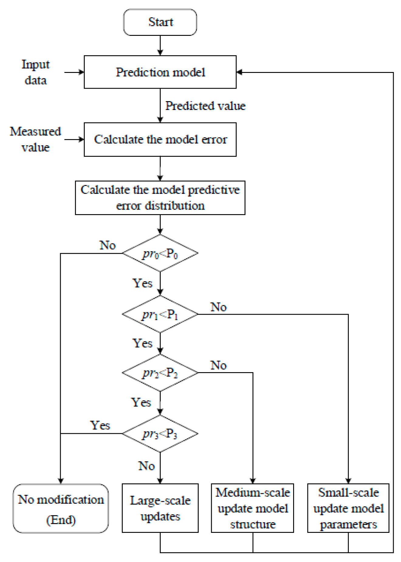
The accuracy of the hybrid model is evaluated via simulation online. The sample interval is selected by sliding the window to maintain the number of samples as ns, and the absolute value of the error is statistically analyzed. If the prediction error of the hybrid model is below a threshold determined by technicians according to the benefit of the process, the model is considered to be accurate. Otherwise, the reason why the model is inaccurate is analyzed, and the model is modified at a different scale according to the variation range of the model error. The modified model is monitored for a time period to ensure that the modification is effective. Otherwise, the modification process continues. The more detailed modification procedure, as shown in Figure 3, is described below.
The prediction error for a single sample is denoted as ε , and the thresholds of the prediction error are ε 0 , ε 1 , and ε 2 , with 0 < ε 0 < ε 1 < ε 2 . In a time period, the numbers of errors in [ 0 , ε 0 ] , [ ε 0 , ε 1 ] , [ ε 1 , ε 2 ] , and [ ε 2 , + ] are denoted as n 0 , n 1 , n 2 , and n 3 , respectively. The probability of the error in the four ranges is calculated in Equation (18).
p r i = n i i = 0 3 n i , ( i = 0 , 1 , 2 , 3 ) .
Suppose that the four thresholds for the probability are P i ( i = 0 , 1 , 2 , 3 ) . Then, the modification is performed according to the relationship between p r i and P i .
If p r 0 P 0 , the model is considered to be accurate, and no modification is needed. If the distribution pr1 has p r 1 P 1 , the error of the prediction model is slightly too large; thus, the requirement of the process is not satisfied. Usually, this is not caused by a large variation of the feed properties. Thus, only the parameters of the sub-models are modified. An improved K-neighbor just-in-time learning algorithm is proposed to retrain the SLFN models for improving the accuracy, which is called “small-scale modification”. Details of the method can be found in Section 3.1.
If the distribution pr2 has p r 2 P 2 , the error of the prediction model is large. Then, structure modification is performed on the SLFN sub-model by using the structure pruning method, and the model is updated. This is called “medium-scale modification”. Details of the method can be found in Section 3.2.
If p r 3 P 3 , the model error is very large, and the variations of the feed properties and the working conditions are considered at the same time. Firstly, all the hybrid SLFN models are modified by updating the model parameters and structure updating. If the model is still not accurate, it is not applicable to the current working conditions, and remodeling is considered. This is called “large-scale modification”.

3.1. Improved K-Neighbor Just-In-Time Learning for Small-Scale Modification

In this section, a small-scale modification method using just-in-time modeling is described. Here, a method is proposed to select a better modeling dataset for the just-in-time method, and the original model is then retrained to update the model parameters. When the just-in-time learning method is used for online modeling, firstly, the samples most similar to the current sample are selected, and then the selected samples are employed to construct a new model or retrain the existing model. The current input sample is denoted as x q ( 1 × n ) , where n is the number of input variables. This is also called a query vector.
The historical input samples are denoted as X ( N × n ) , with i = 1 , 2 , , N , where x i represents the i-th historical input sample with n inputs, which is also called the response vector, and N represents the number of the samples. Then,
x q = ( x q 1 , x q 2 , , x q n ) ,
x i = ( x i 1 , x i 2 , , x i n ) .
The Euclidean distance d q i and the cosine of the vectoral angle cos ( θ q i ) of x q and x i are given as follows:
d q i = j = 1 n ( x q j x i j ) 2 , j = 1 , 2 , , n ,
cos ( θ q i ) = x q x i T x q 2 x i 2 ,
where x i j is the j-th variable of sample x i .
Then, the similarity between the query vector x q and the response vector x i is evaluated to select samples for just-in-time modeling. Usually, the following Equation is used to calculate the similarity [12,13]:
s q i = λ e d q i 2 + ( 1 λ ) cos ( θ q i ) .
In Equation (23), λ [ 0 , 1 ] is an unknown parameter that is usually determined by experience.
According to many studies [12,13,14,15,16,17,18,19,20], the samples used for just-in-time learning significantly affect the performance of the model. In order to improve the quality of the dataset selected for just-in-time learning modeling, a new similarity-evaluation Equation is proposed below.
c q i = cos ( θ q i ) e d q i 2 ,
where c q i represents the similarity of the samples x q and x i , with c q i [ 1 , 1 ] .
When c q i < 0 , the cosine angle of the two samples is large, the similarity is small, and x i is not suitable for just-in-time modeling. When c q i > 0 , the similarity is larger. If c q i is close to 1, the sample x i is selected for just-in-time modeling.
The first k samples in descending order of the similarity are selected for just-in-time modeling, which can be expressed as follows:
Ω k = { ( ( x 1 , y 1 ) , ( x 2 , y 2 ) , , ( x k , y k ) ) | c q 1 > c q 2 > > c q k } .
Furthermore, the modeling samples can be optimized in a principal component analysis (PCA) model. From the viewpoint of the correlation among variables, Q is described as distance and T2 is used to guarantee the samples in local region. Then, the two indices are fused to obtain a novel index, whose minimum corresponding to k is the optimal size for local samples [15]. In this study, k = 8. Then, the SLFN models in the model base are retrained using the ELM and the method described in Section 2.2.

3.2. Morris-Based SLFN Structure Pruning for Medium-Scale Modification

For medium-scale modification, the structure of the SLFNs is regulated. Based on the influence of neurons on the output of the model, the pruning is carried out to optimize the network structure. An improved EE is used to evaluate the contribution of a node to the output of the network. If the EE is below a threshold, the node is deleted. When determining the influence of the input layer on the model output, the input variable refers to the input feature (the input of the model). When determining the influence of the hidden layer on the output, the input variable refers to the output of the hidden layer neuron.
The EE was defined by Morris in 1991 [21]. In the standard EE-based Morris pruning method, the values of the input variables are mapped to the range [0, 1], and the space of the input variables is a super-cube with dimension K. If the output y is differentiable, i ( x ) = y / x i can be used as an index to evaluate the influence of the input variable x i on the output y. Then, i ( x ) may be equal to 0 or a nonzero constant for all input vectors x . It may also be a non-constant function of x i or one or more x i ( j i ) . These situations correspond to four cases where the influence of x i on y can be ignored, is linearly addable, or is nonlinear and depends on other variables.
We know that all the input values are in the range [0, 1]. The input values are discretized, and the input variable x i is set equal to one of the values in { 0 , 1 / ( p 1 ) , 2 / ( p 1 ) , , 1 } , where p is an even number determined by experience.
The EE of x i is defined as
d i ( x ) = [ y [ ( x 1 , x 2 , , x i 1 , x i + Δ , x i + 1 , , x k ) y ( x ) ] / Δ ,
where ∆ is a predetermined multiple of 1 / ( p 1 ) .
That is, one EE value is obtained by running the model twice. The first time, the value of the input variable x j ( j = 1 , 2 , 3 , , k ) can be randomly selected, and, the second time, the input value should have an increment of ∆. Then, the significance of the input to the output can be determined by running the model for a number of times proportional to k or k 2 . For each input, numerous p k 1 ( p Δ ( p 1 ) ) EE values are obtained. In the Morris method, it is assumed that the “basic factor (EE)” obeys a certain distribution Fi. The mean quantifies the individual effect of the input on the output, whereas the standard deviation estimates the combined effects of the input due to nonlinearities or interactions with other inputs. These sensitivity measures can be used to rank the inputs according to their relative importance and determine non-influential parameters that may be fixed in subsequent model calibration.
In the standard EE-based Morris pruning method, the input values of a variable must be mapped to the range [0, 1], and the distribution of the input value is usually uniform [42,43]. However, in practice, the value of a variable may vary in a large range and be distributed nonuniformly. Mapping all the values in a large range to the range [0, 1] may result in an unreasonable sample density. Additionally, different input variables may have different types of distributions. In such cases, the standard EE-based Morris pruning method is not suitable. Thus, herein, an improved EE is proposed.
The input variables are denoted as x = [ x 1 , x 2 , , x k ] , and the output variable is denoted as y, where k is the number of input variables. Suppose that there is only one output. The range of the i-th input variable x i is denoted as [ a i , b i ] , and different variables have different types of distributions.
a b i = b i a i ,
a b m i n = m i n ( a b i ) , i = 1 , 2 , 3 , , k ,
0 < Δ < a b m i n / p ,
b a i = b i Δ a i .
To minimize the number of model evaluations which are required to compute the sensitivity measures, Morris designed a random orientation matrix B* = (Jm,1X* + ( Δ /2)[(2BJm,k) D* + Jm,k]) P*, where B* is constructed using B, B is an m × k strictly lower triangular matrix of ones, Jm,k is an m × k matrix of ones, D* is a k × k diagonal matrix with elements chosen randomly from the set [−1, 1], and P* is a k × k matrix constructed by randomly permuting the columns of a k × k identity matrix. For more information on the sampling design, please refer to References [21,42].
The acquisition of the above matrix is a randomization process. Suppose the two rows of B which differ only in their i-th elements (i = 1, 2, …, k) B ( i ) = [ x 1 x 2 x i 1 x i , 1 x i + 1 x k x 1 x 2 x i 1 x i , 2 x i + 1 x k ] and the result of only the first two stages of the randomization process on these rows, then J2,1X* + ( Δ /2)[(2B(i) − J2,k)D* + J2,k] can be obtained. In this study, for the input variable xi, let li = abi/(p − 1). Then, calculate the probability of xi in the ranges [ai, ai + li), [ai + li ai + 2li), …, [ai + (p − 3) li, ai + (p − 2) li), [ai + (p − 2) li, ai + bai), and [ai + bai, bi]. It is clear that, in any column except the i-th, the two elements are equal and have one of the values in [ai, ai + li, ai + 2li, …, (bi Δ )] and [ai + Δ , ai + li + Δ , ai + 2li + Δ , …, (bi Δ ) + Δ ], and each has equal probability. Then, for an input vector x, the improved EE of the i-th input is defined by Equation (26), but the range of xi is different, that is, xi ∈ [ai,bi] and xibi Δ . Therefore, its scope of application is expanded.
The distribution of the EE of the input x i is denoted as F i , that is, d i ( x ) ~ F i . The number of EE values is 2 k 1 p k , with the distribution F i . Then, by analyzing F i in the same way as the standard EE method does, the significance of the input variable is determined. The number of times that the model must be run for obtaining the EE values should be designed economically to limit the computation time. For more detail, please refer to References [21].
According to the modification strategy, when the accuracy of the hybrid model worsens and p r 2 P 2 , the improved EE-based Morris pruning method is activated to improve the model. The procedure for SLFN structure optimization using the pruning method is as follows:
Step 1: Using Equation (12), determine the weights of all the sub-models. In the sub-models which were never modified, the one with the largest weight is modified.
Step 2: Input the sampling matrix into the sub-model with the largest input weight. Then, calculate the EE value of each hidden-layer neuron and its statistical analysis value.
Step 3: Calculate the mean and standard deviation of the neuronal EE values and optimize the neural-network structure by pruning.
Step 4: Retrain the network model. Then, use the test data to test this model, and calculate the model error again.
Step 5: If the model is still in the medium-scale modification region and there are unpruned sub-models, return to Step 1.

3.3. Large-Scale Modification

When the error of the model is too large and p r 3 P 3 , more process data are collected, and all the models are constructed from the first step.

4. Case Study: Online Simulation Using Industrial Data

In this section, a case study is presented, in which the foregoing modeling method and model-modification strategy are employed for modeling and prediction of the tailings grade in mineral processing. In mineral processing, the particle size in the grinding-classification process, recovery rate, concentrate grade, and tailings grade are key indices. However, in many actual processes, these indices are measured offline, causing delays for process control. Additionally, owing to the complexity of the process and the frequent changes of the feed property, prediction models for the indices using neural networks and other methods cannot adapt to the variation of the process. To solve these problems, online simulation using the proposed AFL–SLFN modeling method and the multiscale modification strategy is used to predict the tailings grade, which can improve the computation and model updating speed and the precision of the model.

4.1. Preprocesing of the Dataset

The froth features, process conditions, ore compositions and grade, concentrate grade, and tailings grade were collected in a bauxite beneficiation plant. Then, Pearson correlation analysis and significance test analysis were performed to reduce data redundancy. The variables with a coefficient larger than 0.25, as shown in Table 1, were used as inputs to predict the tailings grade. That is, 12 input features were selected out of a total number of 26 features. The grade was analyzed every 8 h, and the froth features were obtained online by analyzing froth videos and photographs. According to the flowchart of the process, it takes approximately 10 min for the ore to pass from the first scanning cell to the tailings. Therefore, the froth features between 10 and 20 min before the sampling time of the tailings were averaged and used for prediction of the tailings grade. Finally, 450 groups of data were obtained. Thus, the data covered 150 days of production. Among these data, 360 groups were used as training sets, and the remaining 90 groups were used as test sets.
There are some missing values in the original industrial data due to human causes and mechanical failures. Therefore, an associated K-nearest neighbor (Knn) method was used to interpolate the missing data. Firstly, the candidate input feature related to the input feature corresponding to each missing data value were determined by correlation analysis, and all values of the input features were normalized to be dimensionless. Then K samples nearest to the missing data were determined according to the Euclidean distance between each sample of the candidate input features. The K values were then assigned weights by distance to estimate the missing data.

4.2. Small-Scale Mdoification of Prediction Model for Tailings Grade

R represents the number of sub-models, and H represents the number of hidden nodes. Grid searches of R on {2, 3, …, 9, 12} and of H on {5, 8, 11, 14, …, 50} were performed to identify the optimal values. For selecting the activation function, we firstly set up a base-function pool, including a trigonometric function cluster, logarithmic function cluster, polynomial function cluster, or exponential function, Gaussian function, or mixed function cluster. Each activation function was a base function, and different base functions were used for different activation functions. Then, the base functions were adjusted according to the learning accuracy to obtain an optimal combination of the base functions as activation functions. Each model had different activation functions that were randomly selected from { 1 / ( 1 + e x ) , sin x , 0.5 e x 2 / 10 , e x , cos 2 x }.
The effects of the parameters R and H on the results are presented in Table 2. To test the stability of the models, we conducted these experiments 20 times. The results shown in Table 2 are the stable ones.
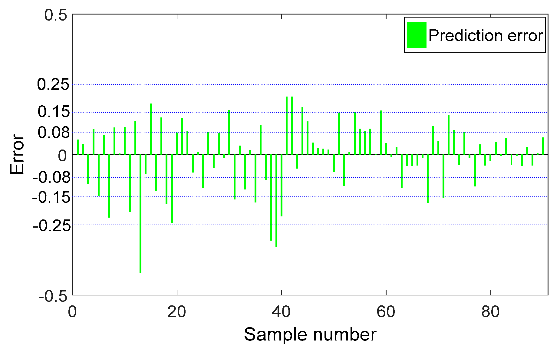
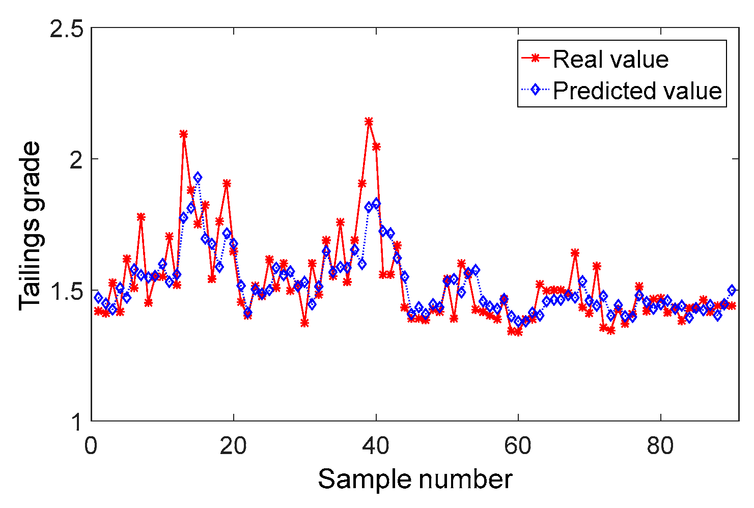
With an increase in the number of hidden-layer neurons and sub-models, model runtime only slightly increased, the accuracy of the model was not always improved; thus, the parameters R and H were set as six and 25, respectively, which were the optimal values. Using the training data, six SLFN sub-models were obtained by conducting the training six times. Each SLFN model had 25 hidden neurons, and the number of hidden neurons was determined by tests. The prediction results for the test dataset are shown in Figure 4. Here, the prediction results represent the adaptive weighting of the six sub-models. The error of the model was calculated using the measured and predicted values, as shown in Figure 5. There were many points with large errors. Therefore, online modification was necessary.
For model modification, the number of samples in the sliding window n s was set as nine, corresponding to three days of production. According to the requirements of the actual production process and the experiences of the operators and the technicians, the error thresholds ε 0 , ε 1 , and ε 2 were set as 0.08, 0.15, and 0.25, respectively, and the model prediction error probability thresholds P 0 , P 1 , P 2 , and P 3 were set as 0.6, 0.3, 0.3, and 0.6, respectively. Here, 0.08 and 0.15 were values accepted by the technicians in the plant, and other values were set according to experience.
Then, the distribution probability of the model error in different regions was calculated. For the first nine samples, the number of errors in the four regions was four, four, one, and zero, as shown in Table 3. Therefore, for the 10th sample, small-scale modification was needed. The improved just-in-time local modeling method was then used to update the model. In this section, only small-scale modification is considered; medium-scale modification is discussed in the next section. The online modification procedure was as follows:
Step 1: According to the k-nearest theory, the eight closest samples to the query sample were selected from the historical data and used for retraining to obtain six new SLFN sub-models, each having five hidden nodes.
Step 2: The new models were then used to predict the tailings grade of the query sample. The six old models were kept in the model base.
Step 3: The sliding window was moved ahead by one sample, and the prediction errors of the samples in the new window were calculated.
Step 4: According to the distribution of the prediction errors, if modification was needed, the foregoing procedure was repeated to construct new models using the just-in-time method; otherwise, the six old models were used for prediction.
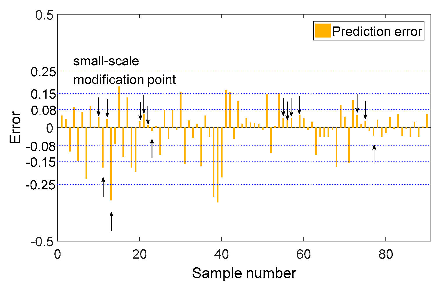
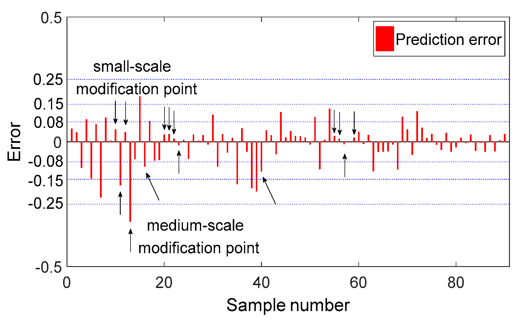
The prediction results and the corresponding errors of the small-scale modified AFL–SLFN model are illustrated in Figure 6 and Figure 7, respectively. In Figure 7, the point with a vertical arrow represents a small-scale modification point.
As shown in Figure 4, Figure 5, Figure 6 and Figure 7, the small-scale modification was effective for tailings grade prediction, and the adaptability of the model was improved. However, for samples 11–20 and 38–44, the prediction errors were large, and the small-scale modification was not adequate. Therefore, medium-scale modification was necessary. Similarly, there were small fluctuations for samples 51–54 and 68–72.

4.3. Medium-Scale Modification of Prediction Model for Tailings Grade

As depicted in Figure 6, the measured value of the tailings grade changed significantly for samples 11 and 38 and deviated for several consecutive samples. According to the distribution of errors listed in Table 3, for sample 16, a medium-scale modification was needed. Thus, the improved Morris pruning method was used to update the sub-model with the largest weight. The pruned model and the other five sub-models were then used to predict the next sample, and the errors were calculated and checked to determine whether further modification was needed. For the 90 samples, two medium-scale modifications were performed. For sample 40, another medium-scale modification was required. Details regarding the pruning method are presented below, taking the second medium-scale modification as an example.
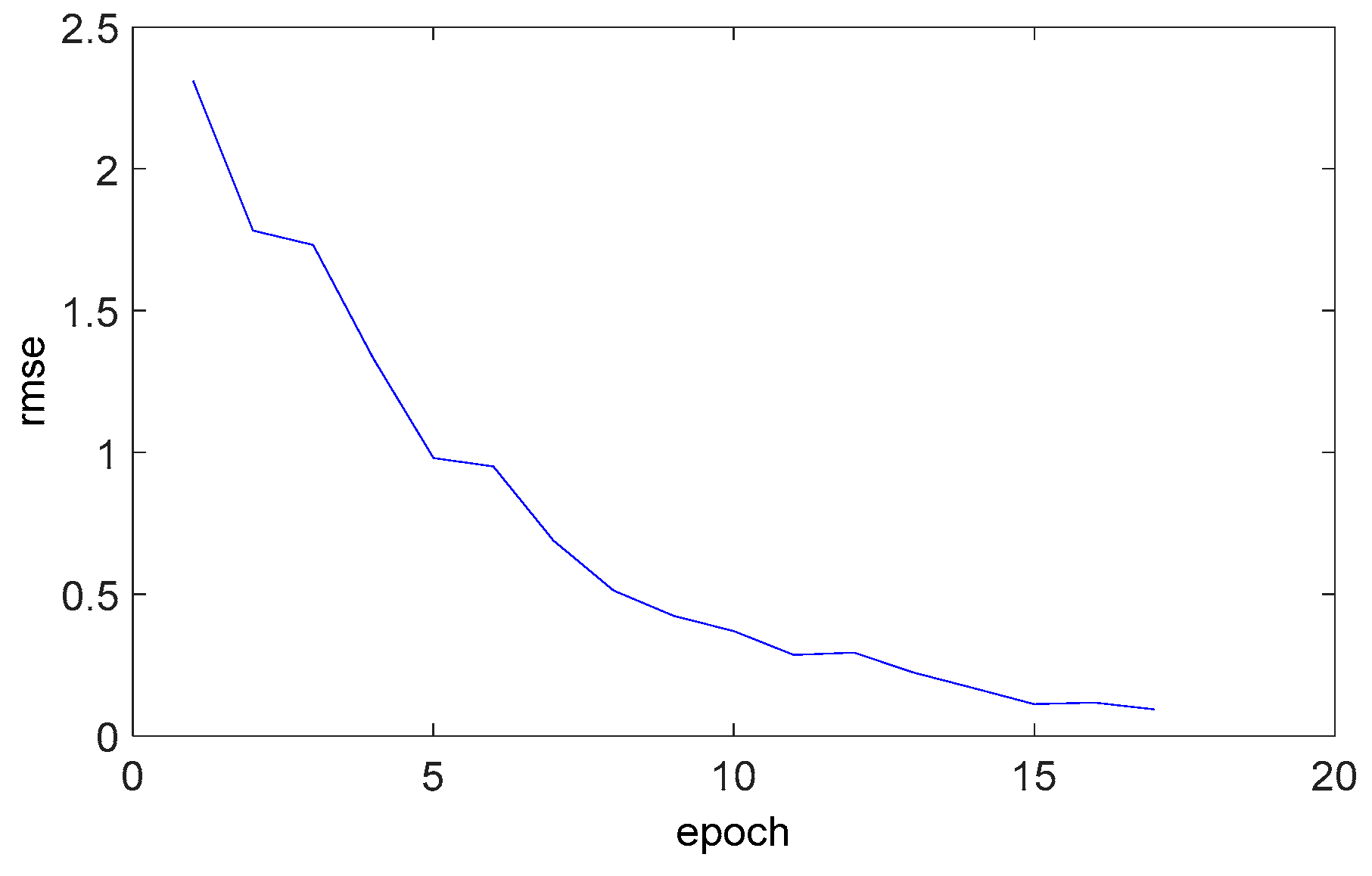
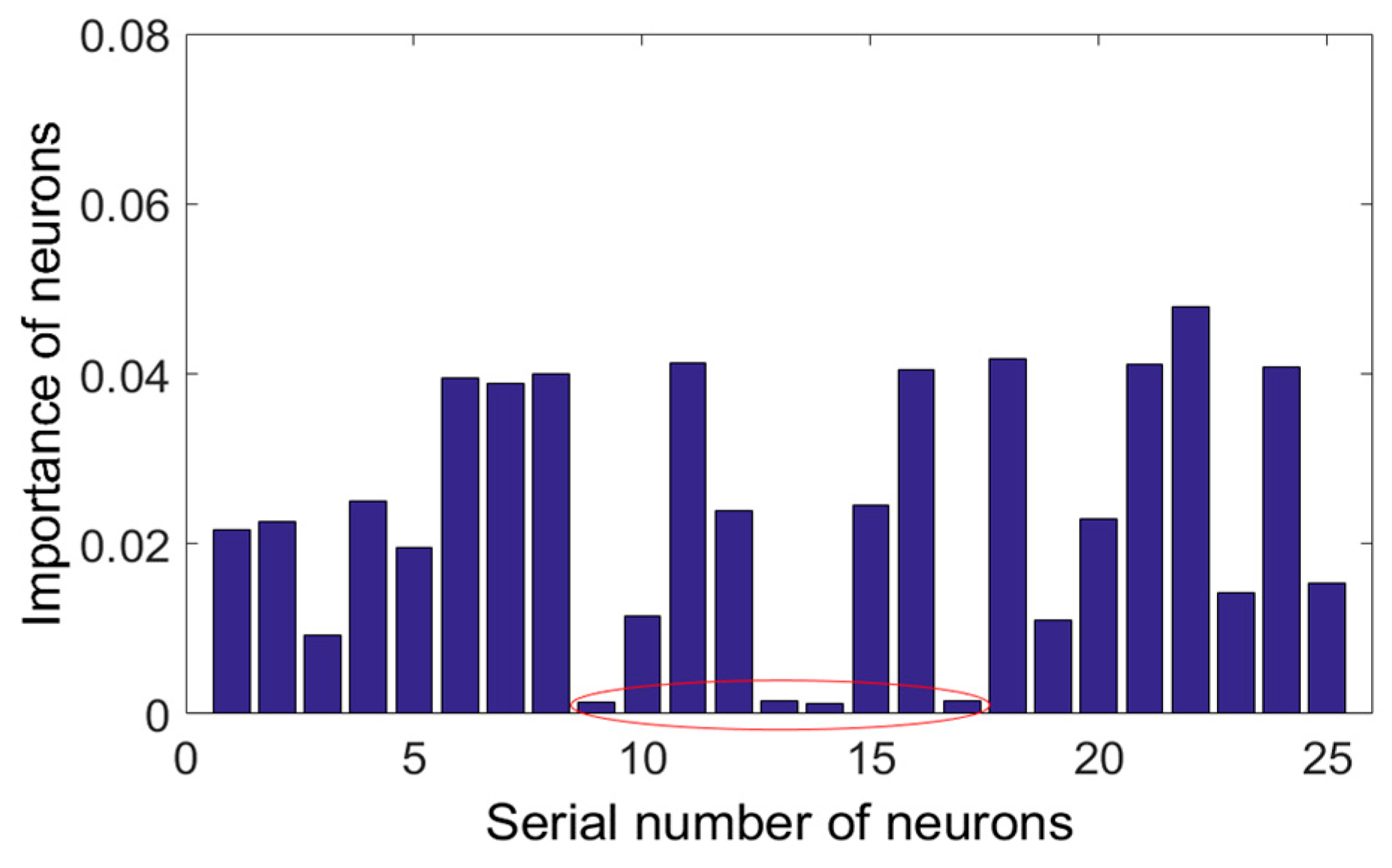
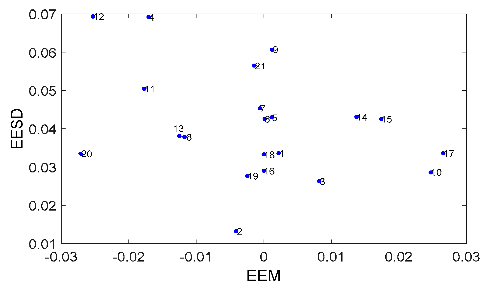
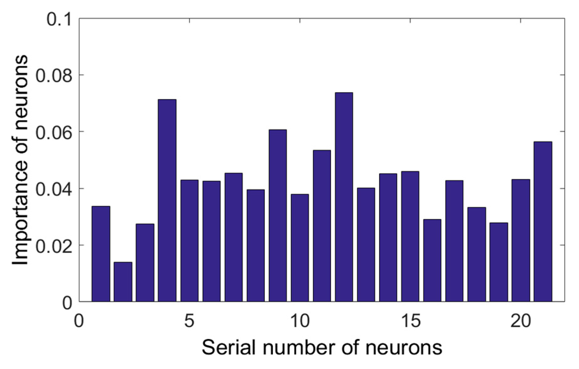
For the second medium-scale modification, the sub-model with the second-largest weight was modified. We knew that there were 25 neurons in the hidden layer of the model. The learning process of the sub-model for the 360 training samples is shown in Figure 8, where the threshold value of the mean square error for training was 0.1. As shown in Figure 8, the training stopped at the 17th iteration. The RMSEs were 0.093518 and 0.099472 for the training and test, respectively. To accurately describe the effect of each hidden-layer neuron on the overall prediction output of the network model, the EE value corresponding to each neuron was calculated using the improved Morris population sampling method. According to the Morris method [21,42,43], the number of EE values of each input was set as r, and then the average of the r EE values was determined. Here, r (≥2) was set randomly. Here, according to experience, the following values were used: r = 6, p = 8, and k = 12. After the model ran once, six independent EE values were obtained for each hidden-layer neuron, and the economy of the model was 12/13. The mean value was taken as the abscissa, and the standard deviation was taken as the ordinate, as shown in Figure 9. To further describe the role of each neuron in the model, the evaluation index is shown in Figure 10.
As shown in Figure 9 and Figure 10, the mean and the standard deviation of the 21 EE values were relatively large, indicating that the corresponding neurons had great influence on the output and could be considered as important neurons. The mean and standard deviation of the ninth, 13th, 14th, and 17th EE values were close to zero. Thus, the corresponding neurons were considered to be unimportant and ignored. Therefore, the ninth, 13th, 14th, and 17th neurons of the hidden layer were deleted. Additionally, as shown in Figure 9, the 22nd input had strong nonlinearity or interaction with other inputs. Hence, the previous 360 samples (counting back from the current query sample) were used as training samples to retrain the pruned sub-model. The simulation results after pruning are shown in Figure 11, Figure 12 and Figure 13.
Following the pruning of the sub-model structure, the raining stopped after the seventh iteration. The training and test RMSEs were 0.071579 and 0.081624, respectively. Thus, the training speed and model accuracy were both improved.
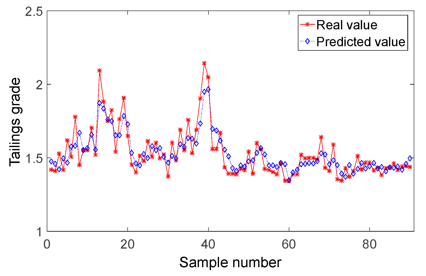
The simulation results of the AFL–SLFN hybrid model with the multiscale modification strategy are illustrated in Figure 14, where small-scale and medium-scale modification was performed by simulating online prediction. The prediction errors are depicted in Figure 15. The distribution of the model errors in all the sliding windows and the modification are presented in Table 3.
As indicated by Table 3, the sample was in the small-scale modification area in the first sliding window, and the local sample set was constructed using the improved K-nearest neighbor just-in-time learning algorithm to predict the 10th test sample. In the fifth sliding window, the error probability of each region was below the threshold value; thus, modification was not necessary, and the initial model was used to predict the 14th test sample. In the seventh sliding window, the sample was in the medium-scale modification area, and the sub-model with the largest weight was selected. The Morris pruning method based on the improved EE value was used to optimize the sub-model structure. After updating the model, the 16th test sample was predicted.
In the eighth sliding window, the error probability of each region was below the threshold; thus, modification was not necessary, and the 17th test sample was predicted using the updated model. By analogy, all predictions were finally obtained.
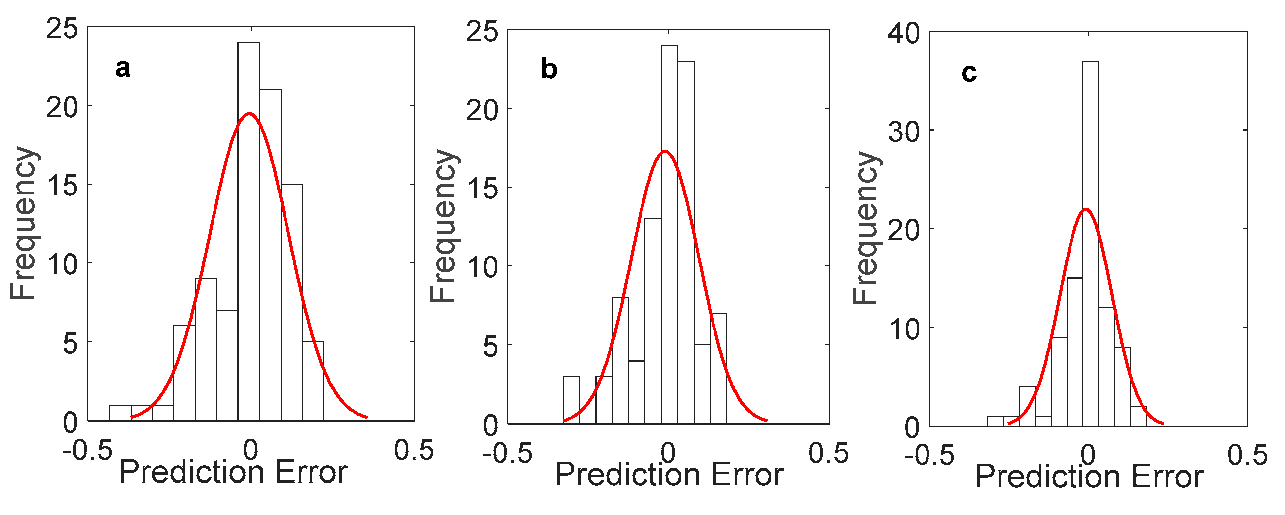
The distributions of the model errors in Figure 5, Figure 7 and Figure 15 are plotted in Figure 16. The statistics of the errors for different modifications, as well as the time consumed (including model modification and prediction), are presented in Table 4.
Figure 16a–c present the error distributions under no modification, small-scale modification, and multiscale modification, respectively. The prediction error had a normal distribution, and the normality of the data was verified by a D-normality test. The results indicated that the models with and without modification were valid. As shown in Figure 16c, the prediction-error distribution for the multiscale modification strategy was the most consistent with the normal distribution, and this strategy yielded the highest accuracy.
Figure 15 and Figure 16 and Table 4 indicate that the hybrid model with only small-scale modification improved the model accuracy significantly. However, the model with multiscale modification tracked the process dynamics with higher accuracy than that with only small-scale modification. In the online modification process, the improved just-in-time local modeling method had to reselect the sample, the medium-scale modification process required pruning, and both of them had to retrain the model. Thus, the computation time increased for the multiscale modification. However, owing to the high speed of the ELM, the runtime of the prediction model did not change significantly. Thus, the model had stronger dynamic adaptability and higher prediction accuracy under the joint action of the small-scale and medium-scale modification strategy and could predict the flotation grade accurately in a long and stable manner.

4.4. Model Comprasion

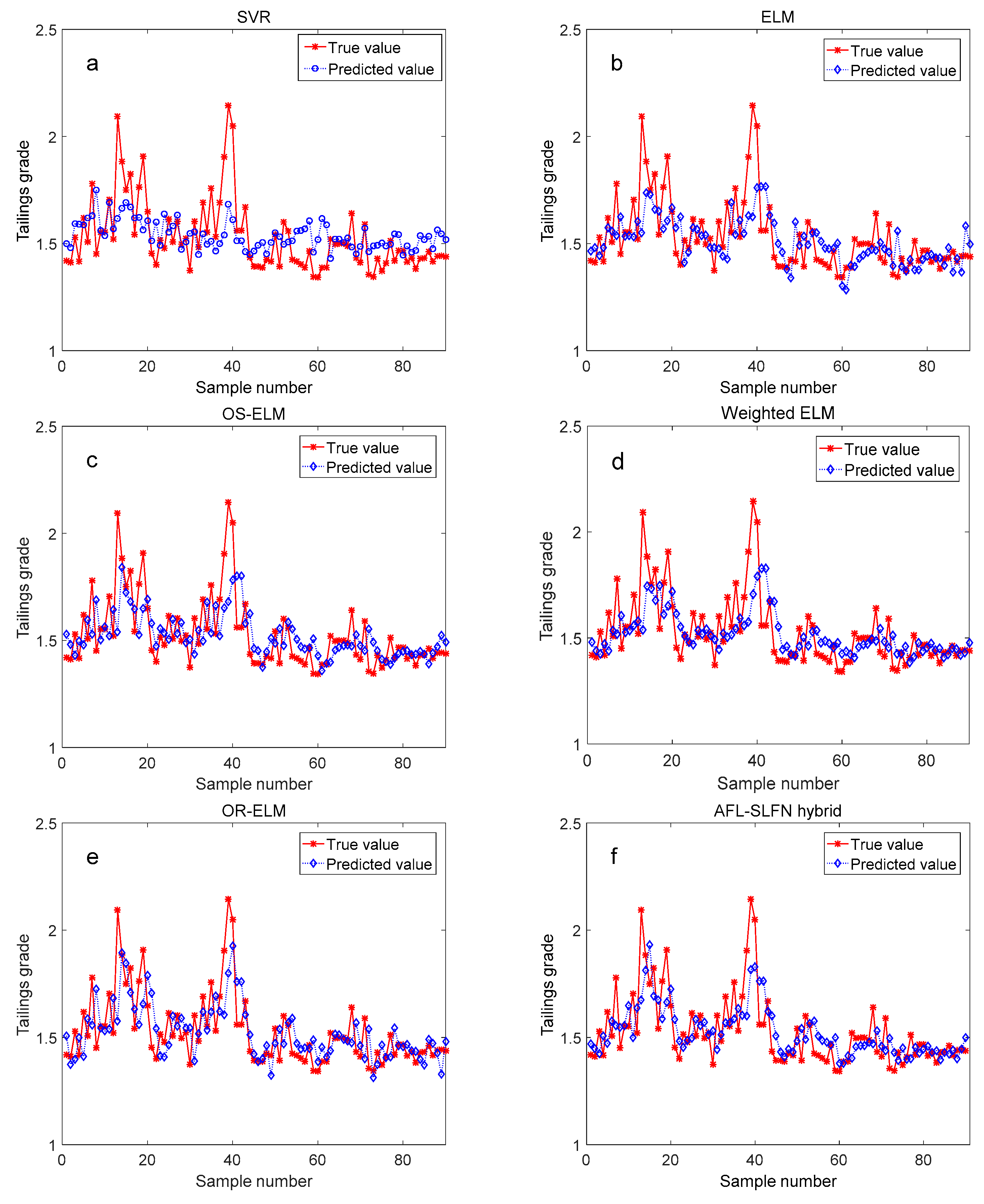
To better demonstrate the capability of the proposed model, its performance was compared with that of state-of-the art algorithms, including support vector regression (SVR), the ELM, the online sequential ELM (OS-ELM) [44], the weighted ELM [45], and the online recurrent ELM (OR-ELM) [46]. In the following experiments, we used the sigmoid function as the activation function of the basic ELM. Grid searches of C (tradeoff constant) on {21, 22, 23, …, 215, 216} for the weighted ELM and of L (hidden-layer nodes) on {5, 10, 15, 20, 25, …, 50} were performed to identify the optimal values for all the models. For the SVR model, the RBF kernel was used. The kernel-function parameters were determined using the approach described in Reference [47]. The regularization parameter was set as four, and the kernel-function parameter was set as 1.0. The prediction results of the proposed model and the other models are illustrated in Figure 14 and Figure 17.
Table 5 presents the prediction performances of all the models according to the following performance metrics: the RMSE, MRE, R2, and Time. Clearly, the AFL–SLFN hybrid model with modification achieved the best outcomes: RMSE = 0.0845, MRE = 0.0361, and R2 = 0.8748. Regarding the runtime, because the proposed method involved a dynamic online modification process, the overall prediction time was longer than that of the static model, but the difference was negligible for the 8-h tailings grade test time.

5. Conclusions

An adaptive weighted hybrid intelligent modeling method with a multiscale online modification strategy for the prediction of industrial-process indices was proposed and verified. The hybrid modeling method is based on an SLFN using an ELM and activation-function learning, where different combinations of base functions are used as activation functions. Thus, the network parameters are trained quickly, and optimization of the structure is convenient. Considering the model mismatch caused by the process dynamics and the instability of the feed properties in industrial processes, a multiscale modification strategy for online estimation was proposed. In this strategy, an improved just-in-time method is used for local modeling, i.e., small-scale modification. The weight distribution of the Euclidean distance and the cosine information do not need to be considered, and the reliability of the local modeling dataset is enhanced. An improved EE-based Morris pruning method is used for optimizing the sub-model parameters and structure, i.e., medium-scale modification. Here, the mapping range and the distribution of input variables can be generalized; thus, the model structure can be optimized conveniently. The method was compared with other state-of-the-art methods via a simulation using preprocessed industrial data. The results indicated that the proposed method can achieve higher accuracy and better adaptability. Meanwhile, due to the model, the modification was done by simulating continuous industrial production, and it can be concluded that the generalization of the model with modification is reasonable.
In this study, only pruning was used for the modification of the network structure. However, sometimes, neurons must be added to the networks. Additionally, adaptively increasing or decreasing the number of input variables and neurons should be investigated for achieving the optimal network structure. Thus, future work will continue to focus on optimizing the network structure.

Author Contributions

Formal analysis, H.Z.; investigation, X.W., Y.W., and S.Y.; methodology, H.Z. and S.Y.; resources, X.W., Y.W., and S.Y.; supervision, X.W.; writing—original draft, H.Z.; writing—review and editing, H.Z. and X.W. All authors read and approved the final version of the manuscript.

Funding

This research was supported by the National Natural Science Foundation of China (No. 61590921), the National Natural Science Foundation of China (No. 61673401 and 61273187), the 111 project (No. B17048), and the Fundamental Research Funds for the Central Universities of Central South University (No. 2018zzts542).

Conflicts of Interest

The author declares no conflicts of interest.

References

  1. Oubelli, L.A.; Aït Ameur, Y.; Bedouet, J.; Kervarc, R.; Chausserie-Laprée, B.; Larzul, B. A scalable model based approach for data model evolution: Application to space missions data models. Comput. Lang. Syst. Struct. 2018, 54, 358–385. [Google Scholar] [CrossRef]
  2. Yerramilli, S.; Tangirala, A.K. Detection and diagnosis of model-plant mismatch in multivariable model-based control schemes. J. Process Control 2018, 66, 84–97. [Google Scholar] [CrossRef]
  3. Ge, Z.; Chen, X. Dynamic Probabilistic Latent Variable Model for Process Data Modeling and Regression Application. IEEE Trans. Control Syst. Technol. 2019, 27, 323–331. [Google Scholar] [CrossRef]
  4. Abdallah, A.M.; Rosenberg, D.E. A data model to manage data for water resources systems modeling. Environ. Model. Softw. 2019, 115, 113–127. [Google Scholar] [CrossRef]
  5. Mcbride, J.; Sullivan, A.; Xia, H.; Petrie, A.; Zhao, X. Reconstruction of physiological signals using iterative retraining and accumulated averaging of neural network models. Physiol. Meas. 2011, 32, 661–675. [Google Scholar] [CrossRef] [PubMed]
  6. Feng, Y.; Hong, W.; Lei, X.; Ping, W.; Song, Z. Data driven model mismatch detection based on statistical band of Markov parameters. Comput. Electr. Eng. 2014, 40, 2178–2192. [Google Scholar]
  7. Giantomassi, A.; Ippoliti, G.; Longhi, S.; Bertini, I.; Pizzuti, S. On-line steam production prediction for a municipal solid waste incinerator by fully tuned minimal RBF neural networks. J. Process Control 2011, 21, 164–172. [Google Scholar] [CrossRef]
  8. Song, W.; Liang, J.Z.; He, X.L.; Chen, P. Taking advantage of improved resource allocating network and latent semantic feature selection approach for automated text categorization. Appl. Soft Comput. J. 2014, 21, 210–220. [Google Scholar] [CrossRef]
  9. Wallace, M.; Tsapatsoulis, N.S. Intelligent initialization of resource allocating RBF networks. Neural Netw. 2005, 18, 117–122. [Google Scholar] [CrossRef]
  10. Wang, M.; Qi, C.; Yan, H.; Shi, H. Hybrid neural network predictor for distributed parameter system based on nonlinear dimension reduction. Neurocomputing 2016, 171, 1591–1597. [Google Scholar] [CrossRef]
  11. Liu, J.; Luan, X.; Liu, F. Adaptive JIT-Lasso modeling for online application of near infrared spectroscopy. Chemom. Intell. Lab. Syst. 2018, 183, 90–95. [Google Scholar] [CrossRef]
  12. Cheng, C.; Chiu, M.-S. A new data-based methodology for nonlinear process modeling. Chem. Eng. Sci. 2004, 59, 2801–2810. [Google Scholar] [CrossRef]
  13. Ding, Y.; Wang, Y.; Zhou, D. Mortality prediction for ICU patients combining just-in-time learning and extreme learning machine. Neurocomputing 2018, 281, 12–19. [Google Scholar] [CrossRef]
  14. Xiong, W.; Zhang, W.; Xu, B.; Huang, B. JITL based MWGPR soft sensor for multi-mode process with dual-updating strategy. Comput. Chem. Eng. 2016, 90, 260–267. [Google Scholar] [CrossRef]
  15. Fujiwara, K.; Kano, M.; Hasebe, S.; Takinami, A. Soft-sensor development using correlation-based just-in-time modeling. AIChE J. 2009, 55, 1754–1765. [Google Scholar] [CrossRef]
  16. Fujiwara, K.; Kano, M.; Hasebe, S. Development of correlation-based pattern recognition algorithm and adaptive soft-sensor design. Control Eng. Pract. 2012, 20, 371–378. [Google Scholar] [CrossRef]
  17. Yu, A.; Grauman, K. Predicting Useful Neighborhoods for Lazy Local Learning. In Proceedings of the Advances in Neural Information Processing Systems 27: Annual Conference on Neural Information Processing Systems 2014, Montreal, QC, Canada, 8–13 December 2014. [Google Scholar]
  18. Uchimaru, T.; Kano, M. Sparse Sample Regression Based Just-In-Time Modeling (SSR-JIT): Beyond Locally Weighted Approach. IFAC Pap. 2016, 49, 502–507. [Google Scholar] [CrossRef]
  19. Niu, D.; Liu, Y. Modeling hydrometallurgical leaching process based on improved just-in-time learning algorithm. In Proceedings of the 2017 36th Chinese Control Conference (CCC), Dalian, China, 26–28 July 2017. [Google Scholar]
  20. Yuan, X.; Huang, B.; Ge, Z.; Song, Z. Double locally weighted principal component regression for soft sensor with sample selection under supervised latent structure. Chemom. Intell. Lab. Syst. 2016, 153, 116–125. [Google Scholar] [CrossRef]
  21. Morris, M.D. Factorial sampling plans for preliminary computational experiments. Technometrics 1991, 33, 161–174. [Google Scholar] [CrossRef]
  22. Engelbrecht, A.P. A new pruning heuristic based on variance analysis of sensitivity information. IEEE Trans. Neural Netw. 2001, 12, 1386–1399. [Google Scholar] [CrossRef]
  23. Khoshroo, A.; Emrouznejad, A.; Ghaffarizadeh, A.; Kasraei, M.; Omid, M. Sensitivity analysis of energy inputs in crop production using artificial neural networks. J. Clean. Prod. 2018, 197, 992–998. [Google Scholar] [CrossRef]
  24. Ibrahim, S.; Choong, C.E.; El-Shafie, A. Sensitivity analysis of artificial neural networks for just-suspension speed prediction in solid-liquid mixing systems: Performance comparison of MLPNN and RBFNN. Adv. Eng. Inform. 2019, 39, 278–291. [Google Scholar] [CrossRef]
  25. Huang, G.B.; Saratchandran, P.; Sundararajan, N. A generalized growing and pruning RBF (GGAP-RBF) neural network for function approximation. IEEE Trans. Neural Netw. 2005, 16, 57–67. [Google Scholar] [CrossRef] [PubMed]
  26. Hayashi, Y.; Setiono, R.; Azcarraga, A. Neural network training and rule extraction with augmented discretized input. Neurocomputing 2016, 207, 610–622. [Google Scholar] [CrossRef]
  27. Yin, J. A variable-structure online sequential extreme learning machine for time-varying system prediction. Neurocomputing 2017, 261, 115–125. [Google Scholar] [CrossRef]
  28. Henríquez, P.A.; Ruz, G.A. A non-iterative method for pruning hidden neurons in neural networks with random weights. Appl. Soft Comput. 2018, 70, 1109–1121. [Google Scholar] [CrossRef]
  29. Mohammed, M.F.; Lim, C.P. A new hyperbox selection rule and a pruning strategy for the enhanced fuzzy min–max neural network. Neural Netw. 2017, 86, 69–79. [Google Scholar] [CrossRef]
  30. Han, H.-G.; Zhang, S.; Qiao, J.-F. An adaptive growing and pruning algorithm for designing recurrent neural network. Neurocomputing 2017, 242, 51–62. [Google Scholar] [CrossRef]
  31. Mei, W.; Liu, Z.; Cheng, Y.; Zhang, Y. A MDPSO-Based Constructive ELM Approach With Adjustable Influence Value. IEEE Access 2018, 6, 60757–60768. [Google Scholar] [CrossRef]
  32. Zhang, S.; Liu, Z.; Huang, X.; Xiao, W. A Modified Residual Extreme Learning Machine Algorithm and Its Application. IEEE Access 2018, 6, 62215–62223. [Google Scholar] [CrossRef]
  33. Yang, S.; Wang, Y.; Sun, B.; Peng, K.; Zhang, X. ELM weighted hybrid modeling and its online modification. In Proceedings of the 2016 Chinese Control and Decision Conference (CCDC), Yinchuan, China, 28–30 May 2016; pp. 3443–3448. [Google Scholar]
  34. Yang, S.; Wang, Y.; Wang, M.; He, H.; Li, Y. Active Functions Learning Neural Network. J. Jiangnan Univ. 2015, 6. [Google Scholar]
  35. Huang, G.B. Extreme learning machines: A survey. Int. J. Mach. Learn. Cybern. 2011, 2, 107–122. [Google Scholar] [CrossRef]
  36. Huang, G.B.; Zhu, Q.Y.; Siew, C.K. Extreme learning machine: Theory and applications. Neurocomputing 2006, 70, 489–501. [Google Scholar] [CrossRef]
  37. Yao, L.; Ge, Z. Distributed parallel deep learning of Hierarchical Extreme Learning Machine for multimode quality prediction with big process data. Eng. Appl. Artif. Intell. 2019, 81, 450–465. [Google Scholar] [CrossRef]
  38. Adhikari, N.C.D.; Alka, A.; George, R.K. TFFN: Two hidden layer feed forward network using the randomness of extreme learning machine. In Proceedings of the 2017 International Conference on Intelligent Sustainable Systems (ICISS), Palladam, India, 7–8 December 2017; pp. 852–857. [Google Scholar]
  39. Golestaneh, P.; Zekri, M.; Sheikholeslam, F. Fuzzy wavelet extreme learning machine. Fuzzy Sets Syst. 2018, 342, 90–108. [Google Scholar] [CrossRef]
  40. Zhang, H.; Zhang, S.; Yin, Y. Online sequential ELM algorithm with forgetting factor for real applications. Neurocomputing 2017, 261, 144–152. [Google Scholar] [CrossRef]
  41. Liao, Y.H.; Chou, J.C. Weighted Data Fusion Use for Ruthenium Dioxide Thin Film pH Array Electrodes. IEEE Sens. J. 2009, 9, 842–848. [Google Scholar] [CrossRef]
  42. Lewis, A.; Smith, R.; Williams, B. Gradient free active subspace construction using Morris screening elementary effects. Comput. Math. Appl. 2016, 72, 1603–1615. [Google Scholar] [CrossRef] [Green Version]
  43. Shi, W.; Chen, X. Controlled Morris method: A new distribution-free sequential testing procedure for factor screening. In Proceedings of the 2017 Winter Simulation Conference (WSC), Las Vegas, NV, USA, 3–6 December 2017; pp. 1820–1831. [Google Scholar]
  44. Liang, N.; Huang, G.; Saratchandran, P.; Sundararajan, N. A Fast and Accurate Online Sequential Learning Algorithm for Feedforward Networks. IEEE Trans. Neural Netw. 2006, 17, 1411–1423. [Google Scholar] [CrossRef]
  45. Zong, W.; Huang, G.-B.; Chen, Y. Weighted extreme learning machine for imbalance learning. Neurocomputing 2013, 101, 229–242. [Google Scholar] [CrossRef]
  46. Park, J.M.; Kim, J.H. Online recurrent extreme learning machine and its application to time-series prediction. In Proceedings of the International Joint Conference on Neural Networks, Anchorage, AK, USA, 14–19 May 2017. [Google Scholar]
  47. Al-Musaylh, M.S.; Deo, R.C.; Adamowski, J.F.; Li, Y. Short-term electricity demand forecasting with MARS, SVR and ARIMA models using aggregated demand data in Queensland, Australia. Adv. Eng. Inform. 2018, 35, 1–16. [Google Scholar] [CrossRef]
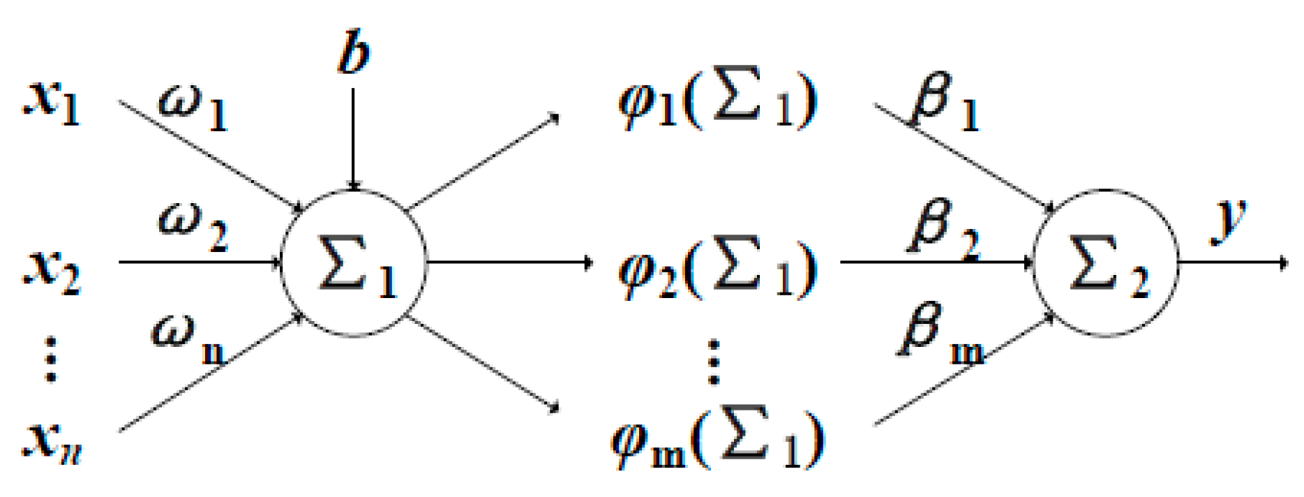
Figure 1. Single-layer feedforward neural network with activation-function learning (AFL–SLFN) with a simple structure.
Processes 07 00893 g001
Figure 2. Hybrid weighted model.
Processes 07 00893 g002
Figure 3. Model-modification strategy.
Processes 07 00893 g003
Figure 4. Prediction results obtained without the modification strategy.
Processes 07 00893 g004
Figure 5. Prediction error for the tailings grade without the modification strategy.
Processes 07 00893 g005
Figure 6. Prediction results obtained using the small-scale modification strategy.
Processes 07 00893 g006
Figure 7. Prediction error for the tailings grade with the small-scale modification strategy.
Processes 07 00893 g007
Figure 8. AFL–SLFN training process.
Processes 07 00893 g008
Figure 9. Distribution of the elementary effect (EE) values in hidden-layer neurons.
Processes 07 00893 g009
Figure 10. Effect of each hidden neuron on the model.
Processes 07 00893 g010
Figure 11. AFL–SLFN training process after pruning.
Processes 07 00893 g011
Figure 12. Distribution of the EE values in the hidden-layer neurons after pruning.
Processes 07 00893 g012
Figure 13. Effect of each hidden neuron on the model after pruning.
Processes 07 00893 g013
Figure 14. Prediction results for the multiscale modification strategy.
Processes 07 00893 g014
Figure 15. Prediction error for the tailings grade with the multiscale modification strategy.
Processes 07 00893 g015
Figure 16. Error distributions for the different modification strategies: (a) error distribution for Figure 5; (b) error distribution for Figure 7; (c) error distribution for Figure 15.
Processes 07 00893 g016
Figure 17. Prediction results for the tailings grade: (a) support vector regression (SVR) model; (b) extreme learning machine (ELM) model; (c) online sequential (OS)-ELM model; (d) weighted ELM model; (e) online recurrent (OR)-ELM model; (f) AFL–SLFN hybrid model.
Processes 07 00893 g017
Table 1. Pearson coefficient and Ps value of input features.
No.FeaturePearson CoefficientSignificance Test (Ps)
1Feeding rate−0.4032622.234 × 10−19
2Na2CO3 addition0.3371951.145 × 10−13
3Roughing dispersant−0.2545341.123 × 10−7
4Cleaner_1 dispersant−0.2985006.705 × 10−11
5Fan frequency for air sparge−0.3198022.251 × 10−12
6Roughing_1 collector−0.3399107.071 × 10−14
7Rough scavenging collector0.3889684.982 × 10−18
8Cleaner scavenging collector0.3729191.363 × 10−16
9Roughing_1 froth depth−0.3295494.342 × 10−13
10Roughing_2 froth depth−0.2897022.517 × 10−10
11Cleaner_1 froth depth−0.2585621.906 × 10−8
12Cleaner_2 froth depth−0.2559402.678 × 10−8
Table 2. Performance comparison among different parameter sets. MRE—mean relative error; RMSE—root-mean-square error.
RHMRERMSER2Time (s)
3100.06530.14630.47951.2163
250.05820.12480.66221.2424
400.06000.12440.66661.2815
6100.06080.13760.59061.2525
250.05830.12110.68701.2883
400.05770.12230.67921.3946
10100.06170.13920.58981.3412
250.05890.12140.68391.3204
400.05910.12300.67031.5452
Table 3. Error distribution in each sliding window.
No.Sliding Window[0, 0.08)[0.08, 0.15)[0.15, 0.25)[0.25, ∞]Query SampleModification Strategy
1Samples 1–9441010Small
2Samples 2–10441011Small
3Samples 3–11342012Small
4Samples 4–12432013Small
5Samples 5–13422114None
6Samples 6–14512115None
7Samples 7–15413116Medium
8Samples 8–16422117None
81Samples 81–89900090None
82Samples 82–909000NoneNone
Table 4. Comparison of the online modification strategies for predicting the tailings grade.
Modification StrategyRMSEMRER2Time (s)
No modification0.12110.05830.68701.2883
Small-scale modification0.10570.04740.78184.6665
Multiscale modification0.08450.03160.87489.1429
Table 5. Comparison of different models for tailings grade prediction. SVR—support vector regression; ELM—extreme learning machine; OS—online sequential; OR—online recurrent; AFL–SLFN—single-layer feedforward neural network with activation-function learning.
ModelRMSEMRER2Time (s)
SVR0.14720.06970.47552.7811
ELM0.14210.06510.54051.0093
OS-ELM0.14050.06340.54731.8993
Weighted ELM0.13800.06120.56441.6771
OR-ELM0.13260.06290.62021.8219
AFL–SLFN hybrid0.12110.05830.68701.2883
AFL–SLFN hybrid with modification0.08450.03610.87489.1429