Dynamic Semi-Quantitative Risk Research in Chemical Plants

Abstract

When a major accident occurs in a chemical industry park, it directly affects the personal safety of operators and neighboring residents and causes major losses; therefore, we should take measures to strengthen the management of chemical industry parks. This article proposes and analyzes a new dynamic semi-quantitative risk calculation model for chemical plants that can be applied digitally. This model provides a sustainable, standardized, and comprehensive management strategy for the safety management of chemical plants and chemical industry park managers. The model and its determined parameters were applied to the safety management of chemical companies within the chemical industry park of Quzhou, Zhejiang Province. From the point of view of the existing semi-quantitative model, the existing problems of the current model are analyzed, the current model is optimized, and a new dynamic semi-quantitative calculation model scheme is proposed. The new model uses an analytical hierarchy process targeting the factors affecting the risks in chemical plants, and chemical plant semi-quantitative dynamic calculation system consisting of the operator, process/equipment, risk, building environment, safety management, and domino effect, and the comprehensive risk of the chemical plant was calculated. The model is ultimately a real-time quantitative value, but its calculation process can compare and analyze the causes of high risk in a chemical plant as they relate to these six factors. Its implementation requires only software, which will greatly help chemical plant safety management.

1. Introduction

Chemical industry parks are built in development zones and are based on the development of oil and chemicals. They have unique inner features, and their most important characteristic is that they are potentially dangerous. Due to the nature of chemical products, chemical industrial parks are potentially high risk: chemical plants are concentrated in the parks, and there are many major hazards such as inflammable, explosive, and toxic chemicals within them. When an accident occurs, the consequences can be very serious. Historical examples include the Bhopal tragedy [1], the Piper Alpha [2], the Flixborough disaster [3], BP Texas City [4], the West Fertilizer explosion [5], the Tianjin explosion, etc. [6] (details of these events are shown in

Table 1. Some major chemical accidents in recent years.

Time	Accident Location	Accident Type	Death Toll	Direct Property Loss
1974.6.1	Flixborough	Chemical explosion	28	unknown
1984.12.2	Bhopal	Chemical poisoning	25,000	$470 million
1988.7.6	Piper Alpha	Chemical explosion	167	$7500 million
2013.4.17	State of Texas	Chemical explosion	35	unknown
2015.8.12	Binhai, Tianjin	Chemical explosion	165	$1098 million

).Therefore, the safety management of chemical industry parks is very important.

To prevent and control major chemical safety accidents, we need to take appropriate measures to strengthen the management of chemical industry parks. There are many factors affecting chemical safety accidents, mainly human, machine, material, method, environment, management, and others; if we can comprehensively monitor and manage these safety factors, we can detect potential safety problems in a timely manner and immediately rectify and improve them to prevent major accidents. Targeted management of the risk level of dangerous chemicals in chemical industry parks can be used to fully mobilize the limited resources of government departments and plants. The focus of such management, rational distribution, is one of the most ideal management tools currently used in chemical industry parks. Therefore, chemical industry parks should implement a combination of key management of major chemical hazards and real-time monitoring.

Comparatively more research has been invested in hazard risk assessment, and quantitative risk assessment methods have been used in the overall risk assessment and safety planning of chemical industry parks, for example, the U.K.’s Canvey Island research project in 1978, Italy’s Ravenna research project in 1979, and the Rijnmond research project in the Netherlands in 1979 [7]. In 2002, the European Union research center launched the ARAMIS(accidental risk assessment methodology for industries) project and provided a comprehensive evaluation system [8,9] as a part of this project. In 2004, Khan F.I, Amyotte P.R proposed the comprehensive essential safety index (I2SI), which consists of two main sub-indices: the risk index (HI) and the underlying safety potential index [10]. Khakzad et al. [11] applied bow-tie and Bayesian network methods in conducting quantitative risk analysis of drilling operations. Abimbola et al. [12] performed safety and risk analysis of a managed pressure drilling operation using Bayesian networks. Goerlandt et al. [13] presented a review focusing on the validation of QRA (quantitative risk analysis) in a safety context. Valerie DE Dianous et al. [14] studied the consequences and causes of all kinds of accidents faced by plants in the chemical industry and emphasized the use of the bow structure diagram method. Christian Delvosalle et al. [15] analyzed the possible accident scenarios for various major hazards. Bahman [16] proposed a new approach, which can predict and assess the impact of an accident in one process unit on the other process units that could be affected. Jonkman S.N et al. [17] gave a model of quantitative risk measures for loss of life and economic damage. Selvik J.T et al. presented and discussed the RCM (reliability centered maintenance) framework to improve risk and uncertainty assessments. The QRA techniques used are based on standard methods, such as fault tree and event tree analysis, but also on more tailor-made methods and approaches to meet the great diversity of processes, hazardous materials, equipment types, and control schemes that characterize the chemical processing industry [18,19,20]. In chemical risk research, governments are constantly exploring the best ways to solve problems via collaboration. Control standards and procedures related to major hazards are promulgated by the United Kingdom, France, the Netherlands, etc. [21,22,23,24,25]. In terms of risk criteria, Kletz [7] proposed that the highest risk of death among residents in the vicinity of chemical facilities is 10⁻⁶ per year, and some companies in the United Kingdom, the United States, and Denmark use this risk standard. According to the risk assessment methods of major hazards and different occasions, the Dutch government has also established reference values for personal and social risks relating to chemical plants [26,27]. A risk index was devised to allow the assessment of the risk level originating from a given installation or site over the affected zone, and a Bayesian network methodology was developed to estimate the total probability of a major accident in a chemical plant [28,29,30,31,32]. The current research detailed above, which is mainly used for chemical industry park planning and analysis, cannot be easily used for the dynamic safety management of existing chemical industry parks; in addition, only the main hazards themselves were considered in these studies, and other major factors that affect safety accidents, such as human, machine, material, method, and environment, were not considered.

To sum up, there are more mature safety assessment methods that have been developed at home and abroad, but these are mainly relatively static assessment methods for the planning of chemical industry parks. For example, Nancy Leveson [33] presented a new accident model founded on basic systems theory concepts. The use of such a model provides a theoretical foundation for the introduction of new unique types of accident analysis, hazard analysis, and accident prevention strategies. Nancy Leveson [34] also described a new method for identifying system-specific leading indicators based on the accident causal relationship of the STAMP (System-Theory Accident Model and Process) model and tools that were intended to be built on the model. There are fewer methods of dynamic assessment generally, and they do not take into account factors beyond the hazards themselves, such as the dynamic process of change in the production and storage of hazards or the combined effects of operators, process, equipment, the building environment, safety management, and the domino effect [35]. The question that remains, and which we address in this paper, is how to carry out dynamic and quantitative assessment of the major hazards in a chemical industry park and provide an assessment result of the dangers in the chemical plants to the park managers promptly and intuitively, so that the park managers can detect the potential safety hazards in time and avoid the occurrence of major safety accidents. The six influencing factors of the model are all dynamic, and each inspection time point has a comprehensive quantitative value. The dynamic form can ensure that the calculated risk value is a real-time quantitative value, which is in line with the actual situation on site and ensures that this research will have great practical significance.

Therefore, this article is based on the research of dynamic semi-quantitative real-time monitoring and management methods for major hazards in chemical industry parks as they relate to the operators, process/equipment, risk, building environment, safety management, and domino effect. We analyze and calculate these six factors and give a dynamic semi-quantitative calculation model of chemical hazards based on an analytical hierarchy process [36]. Using this model, the risk value of each chemical plant in a park can be accurately calculated, and the safety hazards of each chemical plant can be found according to the risk value. Our focus is on the improvement and tracking of safety hazards to reduce the probability of accidents.

2. Using the Analytical Hierarchy Process to Establish a Dynamic Semi-Quantitative Evaluation Model

At present, the mature safety evaluation model is based on the R value. This model only considers the four parameters of the existence of dangerous chemicals (storage) in the major hazards identification of dangerous chemicals (GB18218) specified in the critical mass, which dangerous chemicals these are, the correction coefficient, and the corresponding correction coefficient of major hazards to which the factory personnel are exposed. For a chemical plant in a chemical industrial park, other influence factors, such as the huge number and dense distribution of different kinds of chemical hazards in the park, make it easier for an accident to cause a domino effect. The risk, operators, processes/equipment, building environment, safety management, and other factors in the chemical plant have a great impact on the risk value of the chemical plant. Therefore, we used an AHP (analytical hierarchy process) to conduct dynamic semi-quantitative assessment and monitoring of hazards in chemical plants. At the same time, the influence of the five factors operator, process/equipment, building environment, safety management, and domino effect was added, and the risk value R’ of the danger source was comprehensively calculated. The description of the letters used in the equations in this section is shown in

Table 2. Parameters of the dynamic semi-quantitative evaluation model of chemical hazards.

Parameters:
(1) Hazards calculation parameter
R  risk value
q1,q2, …, qn  The actual quantity (in storage) of each dangerous chemical (tons)
Q1,Q2, …, Qn  Corresponding critical mass (ton)
β1,β2 …, βn  The corresponding correction coefficient
α  Correction factor for number of exposed personnel
R3  R value after optimization
R1  Hazards in the production process
R2  Hazards of the storage tank
q1’,q2’, …, qn’  Quantity of each dangerous chemical online (ton)
Q1’,Q2’, …, Qn’  Corresponding critical mass (ton)
(2) The domino effect calculation parameter
Δp  Blast overpressure (Pa)
p0  Atmospheric pressure (101,325 Pa)
Z  Dimensionless distance
L  The horizontal distance from the target to the source of the blast (m)
E  The total explosive energy source (J)
α’  Equivalent coefficient for vapor cloud, generally 0.04
W1  The mass of fuel in the vapor cloud that actually contributes to the blast shockwave (Kg)
QC  Heat of combustion of the fuel (J/Kg)
q (r)  Radiation flux to the target (W/m2)
q0  Radiation flux on the surface of the fireball, cylindrical tank to take 270 kW/m2, spherical tank to take 200 kW/m2
R0  Fireball radius (m)
r  The horizontal distance from the target to the center of the fireball (m)
W2  Fireball consumption of combustible material (kg)
t  Fireball duration (s)
P  Domino effect probability
Y  Domino effect probability unit
t’  No-fault time
I  Radiation intensity on the target (KW/m2)
V  Equipment volume (m3)
Pblast  The domino effect probability of shockwave
Pheat  The domino effect probability of heat radiation
γ  Domino coefficient
(3) The operator calculation parameter
H1  Personnel qualifying value
H2  Personnel proficiency value
t2  Staff working time at a post
K2  Skilled scale factor
T2  The time required to reach a certain level of proficiency
H3  Personnel stability value
t3  Working hours at the post
K3  Stability ratio coefficient
T3  The time it takes for a person to reach a certain level of operational stability after an accident
H4  Personnel workload value
t4  Personnel work time from work start to work end
K4  Workload ratio factor
T4  Job normal working-class work time, generally taken to be 8 h
M0  Jobs required for the number of workers
N0  The actual number of jobs at the post, and N0 < M0
H5  The reliability value of a single person
Hs  The reliability of the designated post
Hp  The reliability of a single staff member
Hu  The reliability of unit personnel quality
(4) The process/equipment, building environment, and safety management calculation parameter
D  Process/equipment basic score
Xi  The result of process/equipment judgment, yes is 1, no 0
E  Building environment basic score
Yi  The result of building environmental judgment, yes is 1 and no is 0
F  Safety management basic score
Zi  The result of safety management judgment, yes is 1 and no is 0

.

2.1. Establishing a Dynamic Semi-Quantitative Risk Calculation Model for Chemical Hazards

In view of the difficult problem of chemical hazard risk assessment, the fishbone diagram analysis method was used to acquire the six factors that impact the hazard risk, and the six factors were used to construct the model using the analytical hierarchy process. Then, we confirmed the detailed calculation of each indicator on the model, used the forced pair comparison to confirm the weight of each factor, and finally produced the dynamic semi-quantitative hazard risk calculation model, as shown in Figure 1.

2.2. Dynamic Semi-Quantitative Calculation and Analysis of Hazards

2.2.1. Dynamic and Quantitative Calculation of Risk Values for Hazards

According to the requirements of the Provisional Regulations on the Supervision and Administration of Major Dangerous Chemicals, which came into force on 1st, December, 2011, the major hazards are graded by the State Administration of Work Safety (No. 40).

(1)

The classification index uses the actual (stored) amounts of various dangerous chemicals in the unit and their critical amount ratios specified in “Identification of Major Hazard of Dangerous Chemicals” (GB18218); the sum of the ratios of the corrected coefficients is the classification index.

(2)

R value calculation

The R value is calculated as shown in Equation (1), which is from the “Identification of Major Hazard of Dangerous Chemicals” (GB18218). From the calculation of the R value, we can see that the R value actually represents the inherent danger of the hazard, which is formulated by coupling between accident proneness and the seriousness of accident consequences. The correspondence between major hazard levels and R values is shown in

Table 3. The levels of significance of chemical hazards and the corresponding R values.

Chemical Hazard Significance Level	R Value
Level 1	R ≥ 100
Level 2	100 > R ≥ 50
Level 3	50 > R ≥ 10
Level 4	R < 10

.

$$R=\alpha \left({\beta }_1\frac{{\mathrm{q}}_1}{Q_1}+{\beta }_2\frac{{\mathrm{q}}_2}{Q_2}+\dots \dots +{\beta }_{\mathrm{n}}\frac{{\mathrm{q}}_{\mathrm{n}}}{Q_{\mathrm{n}}}\right)$$

(1)

2.2.2. Analysis of Dynamic Semi-Quantitative Hazard Calculation Methods

The R value is currently the traditional classification index for major hazards as it is more intuitive, simple, and easy to calculate; however, its equation does not consider more important factors, only the storage area of the hazard itself, so it is more suitable for small and medium-sized chemical plants. Chemical plants are more concentrated in chemical parks, and because the R value considers too few factors and is not comprehensive enough, it cannot easily reflect all aspects of the characteristics of chemical industry parks. Thus, we need to increase each influence factor and optimize the R value. Using fishbone chart analysis, we can derive the important factors that most affect the risk value of the hazard, as shown in Figure 2.

Hazards in the Pipeline

The current classification of major hazards is calculated based on the stored amount of the hazard in the storage area, which is the main factor affecting the plant risk value. However, hazards in the pipeline are also a great danger. In the event of an accident, these hazards are also more destructive, especially in chemical plants where the output of hazards is relatively large. Therefore, in the calculation of the overall risk value of the chemical plant, this part of the hazards also needs to be taken into account.

Domino Effects in Chemical Industry Parks

The domino effect in a chemical industry park can play an amplifying role in the devastation and damage caused by an accident. This part is also indispensable in the calculation of the risk value of a chemical plant in a chemical park. Valerio Cozzani et al. [35] studied the domino effect in hazards and emphasized the importance of including the domino effect in the calculation of the risk value.

Operator, Equipment, Process, and Environment

“Operator” refers to the operators who use dangerous raw materials and manufacture dangerous products; they are the biggest difficulties in production management and are the focus of discussion in all management theories at present. Operators’ personality traits, ability levels, and education levels are not the same, and their attitude towards the work and awareness of the dangers of the product are not the same; all these have a great impact on the safety of the operation. In the past, a majority of chemical accidents have been due to improper operation by operators. “Equipment” refers to the production of machines, tools, and other auxiliary production equipment. In the production process, whether the equipment is functioning or the tools are good or bad is another factor affecting safety. “Process” refers to the documents, regulations, and systems to be followed in the production process, including process instructions, guidelines for standard processes, production drawings, production schedules, product operating standards, inspection standards, and various operating procedures. If the process is wrong, this will result in a major chemical plant accident. “Environment” refers to the building environment, including the layout of the building and temperature and humidity control. The environment also has a great impact on the occurrence of safety incidents, such as sudden changes in temperature and humidity, which may be a direct result of safety incidents, or improper design of the building environment, which can amplify the scope of and loss resulting from a safety incident. Therefore, in chemical plant risk factor analysis, the operator, equipment/process, and environment cannot be ignored.

Safety Management

Safety management is an important part of production management and is a comprehensive system of science. The object of safety management is the management and control of the status of all people, objects, and the environment in production. It is a kind of dynamic management. Safety and danger exist in the same context in mutual opposition and interdependence. As the movement of things changes, safety and danger are changing all the time, and the fight is reversed. The state of things will tilt toward the victor of the struggle, showing that there is no absolute safety or danger in the movement of things. To maintain the safety status of production, we must take various measures to prevent danger. The risk factors are completely controllable; therefore, in chemical industry park risk factor analysis, corporate safety management is also the top priority.

2.3. Analysis of Influencing Factors in the Dynamic Quantitative Evaluation

2.3.1. Increased Risk of Quantities in the Pipeline

Hazards in storage are a major risk for all chemical plants in a chemical industry park and form a major part of the risk value. The sum of all similar hazards stored on site needs to be calculated. In addition, there is also a need to supplement this with the risk value in the production pipeline, as shown in Equations (2) to (4).

$${\mathrm{R}}_3{=\mathrm{R}}_1{+\mathrm{R}}_2$$

(2)

$$R_1=\alpha \left({\beta }_1\frac{{\mathrm{q}}_1}{Q_1}+{\beta }_2\frac{{\mathrm{q}}_2}{Q_2}+\dots \dots +{\beta }_{\mathrm{n}}\frac{{\mathrm{q}}_{\mathrm{n}}}{Q_{\mathrm{n}}}\right)$$

(3)

$$R_2=\alpha \left({\beta }_1\frac{{\mathrm{q}{}^{\prime }}_1}{Q{{}^{\prime }}_1}+{\beta }_2\frac{{\mathrm{q}{}^{\prime }}_{{}^{\prime }2}}{Q{{}^{\prime }}_2}+\dots \dots +{\beta }_{\mathrm{n}}\frac{{{\mathrm{q}}^{\prime }}_{\mathrm{n}}}{Q{{}^{\prime }}_{\mathrm{n}}}\right)$$

(4)

2.3.2. Domino Effect

The calculation of the domino effect coefficient includes two parameters: the probability of shock domino effect (P_blast) and the probability of thermal radiation domino effect (P_heat). The calculation of the domino effect probability was obtained using a simulation evaluation of accident consequences. By selecting the explosion and fire models as the accident consequence models, we can get the shockwave domino effect probability and the thermal radiation domino effect probability; while there are several accident consequence models for a chemical industry park, the more common are explosion and fire.

(1)

Explosion—blast shockwave overpressure

An explosion is a very sharp physical and chemical change of matter. It is also a phenomenon in which a large amount of energy is quickly released or rapidly transformed into mechanical work in a short time. It is usually achieved by means of gas expansion, which can be physical explosion or chemical explosion according to the nature of the explosion. Physical explosion is a phenomenon in which the material state parameters (temperature, pressure, and volume) change rapidly and emit large amounts of energy and work externally in an instant. Chemical change is the rapid transformation of a substance from one chemical structure to another chemical structure, releasing a large amount of energy and doing work externally. The main types of explosion models are blasting energy from compressed gas containers, blasting energy when all of the media are liquid, blasting energy of liquefied gases, and high-temperature saturated water, steam cloud explosions, and shockwave overpressure.

Overpressure on the shockwave front in shockwave overpressure models is related to the ability to generate shockwaves and is also related to the distance from the explosion center. Shock overpressure can be calculated as shown in Equations (5) to (7).

$$\frac{\Delta p}{P_0}=0.137Z^{-1}+0.119Z^{-2}+0.269Z^{-1}-0.019$$

(5)

$$Z=L•{\left(\frac{P_0}{E}\right)}^{\frac{1}{3}}$$

(6)

$$E=1.8\alpha {}^{\prime }{W}_1{Q}_C$$

(7)

(2)

Fire—thermal radiation

There are two main types of fire assessment: pool fire and vapor explosion (BLEVE).

Liquid leaks generally cause pool fire, the damage from which is mainly thermal radiation. If the heat radiation acts on containers and equipment, especially liquefied gas containers, the internal pressure will rapidly rise, causing the container and equipment to rupture; if heat radiation acts on combustibles, it ignites them; and if heat radiation is applied to personnel, it can cause burns and death. Vapor explosion refers to the sudden boiling of liquid generated by massive overheating causing an explosive boiling phenomenon. The BLEVE acronym stands for “boiling liquid expanded to vapor explosion”, but this is too cumbersome, so it is simplified to “vapor explosion”. According to the characteristics of dangerous chemicals in a chemical industry park, we selected the vapor explosion (BLEVE) model. The thermal radiation flux of this model is calculated as shown in Equations (8) to (10).

$$\mathrm{q}\left(\mathrm{r}\right)=\frac{{\mathrm{q}}_0{R}_0{}^2\mathrm{r}\left(1-0.058\mathrm{lnr}\right)}{{\left(R_0{}^2+r^2\right)}^{3/2}}$$

(8)

$$R_0=2.9W_2{}^{1/3}$$

(9)

$$t=0.45W_2{}^{1/3}$$

(10)

(3)

The accident domino effect threshold

In order to judge whether a domino effect will occur after a major accident occurs, threshold values of the relevant physical parameters characterizing the damage effect are generally selected for determination. If the calculation result of the related physical parameter exceeds the threshold value, a domino effect is considered to be caused.

• Thermal radiation domino effect threshold

The threshold of heat radiation for atmospheric pressure vessels over more than 10 min is 15 kW/m², and the threshold for thermal radiation for pressure vessels over more than 10 min is 50 kW/m²; these were given by Valerio Cozzani et al. [37]. The setting of these thresholds has been approved by other international scholars, and this article also adopts these thresholds.

b.

Shock wave domino effect threshold

Along with the thresholds for the domino effect from thermal radiation, Valerio Cozzani et al. [37] gave destruction thresholds for atmospheric pressure vessels, pressure vessels, long vessels, and small vessels, respectively, of 22 kPa, 16 kPa, 31 kPa, and 37 kPa. The setting of these thresholds has been approved by other international scholars, and this article also adopts these thresholds.

(4)

Domino effect probability

The domino effect probability formula calculates the probability of damage to equipment based on the probability function method for empirical data, as shown in Equation (11). The most common equipment failure probability models are shown in

Table 4. Commonly used equipment failure probability models.

Physical Factors	Container Type	Threshold	Probability Calculation Equations
Overpressure	Atmospheric pressure	22 kPa	Y = −18.96 + 2.44lnPs
	Pressure	16 kPa	Y = −42.44 + 4.33lnPs
	Long type	31 kPa	Y = −28.07 + 3.16lnPs
	Small type	37 kPa	Y = −17.79 + 2.18lnPs
Heat radiation	Atmospheric pressure	More than 10 m,15 W/m2	Y=12.54 − 1.847lnt’
			lnt’ = −1.128lnI − 2.667 × 10−5V + 9.877
	Pressure	More than 10 m, 50 W/m2	Y=12.54−1.847lnt’
			lnt’ = −0.947lnI + 8.835V0.032

.

$$P=\frac{1}{\sqrt{2\pi }}{\displaystyle {\int }_{-\infty }^{Y-5}{e}^{-\raisebox{1ex}{$x^2$}\!\left/ \!\raisebox{-1ex}{$2$}\right.}}dx$$

(11)

(5)

Domino effect coefficient

The value of the domino coefficient γ considers three aspects:

(1)

Domino effect forms, including thermal radiation and shock wave overpressure;

(2)

The probability of a domino effect;

(3)

The number of units that may have a secondary accident affected by the domino effect.

The probability of the domino effect can be obtained by simulating and predicting the accident consequence of major hazards, the principle of maximum risk, and the principle of probability summation of the forecasting process. Thus, the calculation of γ can be obtained as shown in Equation (12):

$$\gamma ={\displaystyle {\prod }_{i=1}^n\left(1+P_{blast}\right)){\displaystyle {\prod }_{k-1}^n\left(1+P_{heat}\right)}}$$

(12)

where i is an accident that occurred in major hazards, causing a second accident in neighboring plant i; k is an accident that occurred in major hazards, causing a second accident in adjacent plant k.

The equations in Section 2.3.2 is from the paper by Valerio Cozzani et al. [37].

2.3.3. Operator

Based on the analysis of human behavior characteristics in the system, the group quality of operators in dangerous positions in industrial facilities was evaluated from the aspects of the eligibility, proficiency, stability, and workload of the operators.

(1)

Personnel eligibility

Dangerous chemicals positions must be certified posts; for those with certificates, we set H₁ = 1; for those not licensed, H₁ = NA (empty value).

(2)

Personnel proficiency

The personnel proficiency was calculated as shown in Equation (13).

$$H_2=1-\frac{1}{k_2\left(\frac{t_2}{T_2}+1\right)}$$

(13)

(3)

Personnel stability

The personnel stability was calculated as shown in Equation (14).

$$H_3=1-\frac{1}{k_3\left[{\left(\frac{t_3}{T_3}\right)}^2+1\right]}$$

(14)

(4)

Personnel workload

If a post should have M₀-many personnel working but in fact has only N₀ people, withM₀>N₀, the working hours should be converted. Therefore, the personnel workload was calculated as shown in Equation (15).

$$H_4=1-k_4{\left[\frac{t_4\left(\frac{M_0-N_0}{M_0}+1\right)}{T_4}-1\right]}^2$$

(15)

(5)

Reliability of individual operators

The reliability of individual operators was calculated as shown in Equation (16).

$$H_5=H_1{H}_2{H}_3{H}_4$$

(16)

(6)

The quality of the operator assigned to the post

The work in a position can be performed by a group of people. Suppose there are N-many people who can operate in the same place (they will work in the same place at different times). Since the relationship between these N individuals is neither “serial” nor “parallel”, the reliability of the designated operator was averaged. Therefore, the reliability of the qualifications of the designated operators was calculated as shown in Equation (17):

$$H_S=\frac{{\displaystyle \sum _{i=1}^N{H}_{5i}}}{N}$$

(17)

where i is the ith person; N is the total number of operators for the same position at different time periods.

(7)

The reliability of the quality of a single post

The reliability of the quality of a single post was calculated as shown in Equation (18):

$$H_p=\underset{i=1}{\overset{n}{\Pi }}{H}_{si}$$

(18)

where i is the ith person; n is the number of people working on a job.

(8)

Unit operator quality of reliability

The unit operator quality of reliability was calculated as shown in Equation (19):

$$H_u=1-\underset{i=1}{\overset{m}{\Pi }}\left(1-H_{pi}\right)$$

(19)

where i is the ith post; m is the number of jobs in a unit.

The equations in Section 2.3.3 is from the “Eighth Five-Year Plan” of China’s national science and technology research topic, which is “Study on Identification and Evaluation Technology of Flammable, Explosive and Toxic Major Hazards”.

2.3.4. Process/Equipment Rating Scale

The process/equipment rating scale comes from the “Eighth Five-Year Plan” of China’s national science and technology research topic, which is “Study on Identification and Evaluation Technology of Flammable, Explosive and Toxic Major Hazards”. The process/equipment used in the hazardous areas in the chemical plant mainly involves the 13 items shown in

Table 5. Chemical hazard process/equipment rating scale.

Number	Item	Content(Keywords)	Score (D)	Xi
1	Equipment maintenance (or)	1. Strict, 2. Basic	8, 6	X11, X12
2	Explosion-proof device (and)	1. Explosive itself, 2. Explosion-proof membrane	24, 11	X21, X22
3	Inert gas protection(or)	1. Continuous, 2. Sufficient	13, 15	X31, X32
4	Emergency cooling (or)	1. More than 10 min, 2. About 10 min	10, 12	X41, X42
5	Emergency Power Supply (or)	1. Multi-channel power supply, 2. Generator set	12	X51, X52
6	Electrical explosion-proof(or)	1. Flameproof, 2. Increased safety, 3. Intrinsically safe, 4. Positive pressure, 5. Oil-filled, 6. Sand-filled, 7. No spark, 8. Explosion-proof, 9. Dust Explosion-proof	7	X61, X62, X63, X64, X65, X66, X67, X68, X69
7	Anti-static (and)	1. Less production, 2. Leakage, 3. Neutralization, 4. Shielding, 5. Smooth surface	7	X71, X72, X73, X74, X75
8	Lightning protection (and)	1. Less production, 2. Leakage, 3. Neutralization, 4. Shielding, 5. Smooth surface	7	X81, X82, X83, X84, X85
9	Device for preventing fire (and)	1. Flame arrester, 2. Fluid seal, 3. Others	12	X91, X92, X93
10	Process parameter control (or)	1. A set, 2. Parallel and manual, 3. Parallel and automatic	11	XA1, XA2, XA3
11	Leak detection device and response(or)	1. Alarm and confirmation, 2. Alarm and protection	11, 15	XB1, XB2
12	Fault alarm and control device (and)	1. Cut off, 2. Control valve, 3. Vibration and alarm, 4. Vibration and protection, 5. Others	11, 11, 10, 13, 10	XC1, XC2, XC3, XC4, XC5
13	Accident emissions and treatment (and)	1. Safety, 2. Outside the unit, 3. Emergency ventilation duct, 4. Double jacket, 5. Protective dike	11, 13, 13, 14, 11	XD1, XD2, XD3, XD4, XD5

. Each item has several sub-items, and the score of each sub-item may be different. There is a need for comprehensive conversion, here given by the rules of each score sheet (sub-item content is reflected in keywords, Table 5).

2.3.5. Building Environment Rating Scale

The building environment rating scale comes from the “Eighth Five-Year Plan” of China’s national science and technology research topic, which is “Study on Identification and Evaluation Technology of Flammable, Explosive and Toxic Major Hazards”. The building environment of the hazardous area in the chemical plant mainly involves the five items in

Table 6. Chemical hazard building environment rating scale.

Number	Item	Content(Keywords)	Score (E)	Yi
1	Ventilation plant	Full ventilation	6	Y11
2	Pressure relief (or)	1. Auto window, 2. Safety hole, 3. Other	8	Y21, Y22, Y23
3	Monitoring device (and)	1. Control room, 2. Surveillance, 3. Troubleshooting	10, 12, 18	Y31, Y32, Y33
4	Plant structure (and)	1. Reasonable classification, 2. Fire resistance, 3. Fire prevention distance, 4. Explosion protection, 5. Escape port	5	Y41, Y42, Y43, Y44, Y45
5	Industrial sewer (and)	1. Industrial sewer, 2. Oil trap	5	Y51, Y52

. Each item has several sub-items, and the score of each sub-item may be different. Comprehensive conversion is given by the rules of each score sheet (sub-item content is reflected in keywords, Table 6).

2.3.6. Safety Management Rating Scale

The safety management rating scale comes from the “Eighth Five-Year Plan” of China’s national science and technology research topic, which is “Study on Identification and Evaluation Technology of Flammable, Explosive and Toxic Major Hazards”. The safety management used in the hazardous area in the chemical plant mainly involves the 10 items shown in

Table 7. Chemical hazard safety management rating scale.

Number	Item	Content(Keywords)	Score (F)	Zi
1	Safety production responsibility system	1. Director, 2. Deputy director, 3. Other deputy director, 4. Chief engineer, 5. Head of department, 6. Director of the workshop, 7. Team leader, 8. Operator, 9. Union leader	1.11	Z11~Z19
2	Safety education	1. New workers, 2. Special workers, 3. New technologies, 4. Returning workers, 5. New jobs, 6. Middle-level cadres, 7. Team leaders, 8. All staff	1.25	Z21~Z28
3	Safety technical measures plan	1. Plan, 2. Specific funds, 3. Responsible person, 4. Target value	2.50	Z31~Z34
4	Safety inspection	1. Regular, 2. Frequent, 3. Dedicated, 4. Professional, 5. Seasonal, 6. Holidays, 7. Focus	1.43	Z41~Z47
5	Safety rules and regulations	1. Rewards, 2. On-duty, 3. Operational procedures, 4. Management, 5. Approval, 6. Hazard, 7. Protection, 8. Electricity, 9. Overtime, 10. Ignition, 11. Inspection, 12. Leakage prevention, 13. Signs	0.77	Z51~Z5D
6	Safety management agencies and personnel	1. Committee, 2. Agency, 3. Part-time management, 4. Part-time employee insurance, 5. Supervisor	2.00	Z61~Z65
7	Statistical analysis of accidents	1. Record, 2. Analyze 3. Statistics	3.33	Z71~Z73
8	Hazard assessment and rectification	1. Safety evaluation, 2. Hierarchical management, 3. Restructuring, 4. Important management	2.50	Z81~Z84
9	Emergency plans and measures	1. Command, 2. Procedure, 3. Plan, 4. Device, 5. Safety exit, 6. Emergency equipment, 7. Communication, 8. Service organization, 9. Exercise	1.11	Z91~Z99
10	Fire safety management	1. Committee, 2. Responsibility, 3. Inspection, 4. Account, 5. Mark, 6. Plane paper, 7. Fire protection, 8. Fire suppression, 9. Communication, 10. Exercise	1.00	ZA1~ZAA

. Each item has several sub-items, and the score of each sub-item may be different. Comprehensive conversion is given by the rules of each score sheet (sub-item content is reflected in keywords, Table 7).

2.4. Constructing a Dynamic Semi-Quantitative Calculation Model for Chemical Hazards

Any one system includes two parts: one is the thing itself, and the other is an important factor affecting it. The important factors affecting chemical hazards are the domino effect, operators, process, equipment, the building environment, and safety management. This article focuses on the” domino effect, operator, process/equipment, building environment, and safety management” system, using a dynamic semi-quantitative system composed of the five parts of the system. The influence coefficient of each index factor can then be calculated, and we can finally calculate the risk value of the hazards.

At the same time, as this article summarizes the previous valuable experience and the current actual situation, we propose setting six first-level indicators (a hazard risk factor, domino effect factor, operator factor, process/equipment factor, building environment factor, and safety management factor) and a total of 42 secondary indicators of the risk value of dangerous chemical hazards to be used to carry out dynamic semi-quantitative calculations, as shown in Figure 3.

3. Index Value Calculations via an Analytical Hierarchy Model

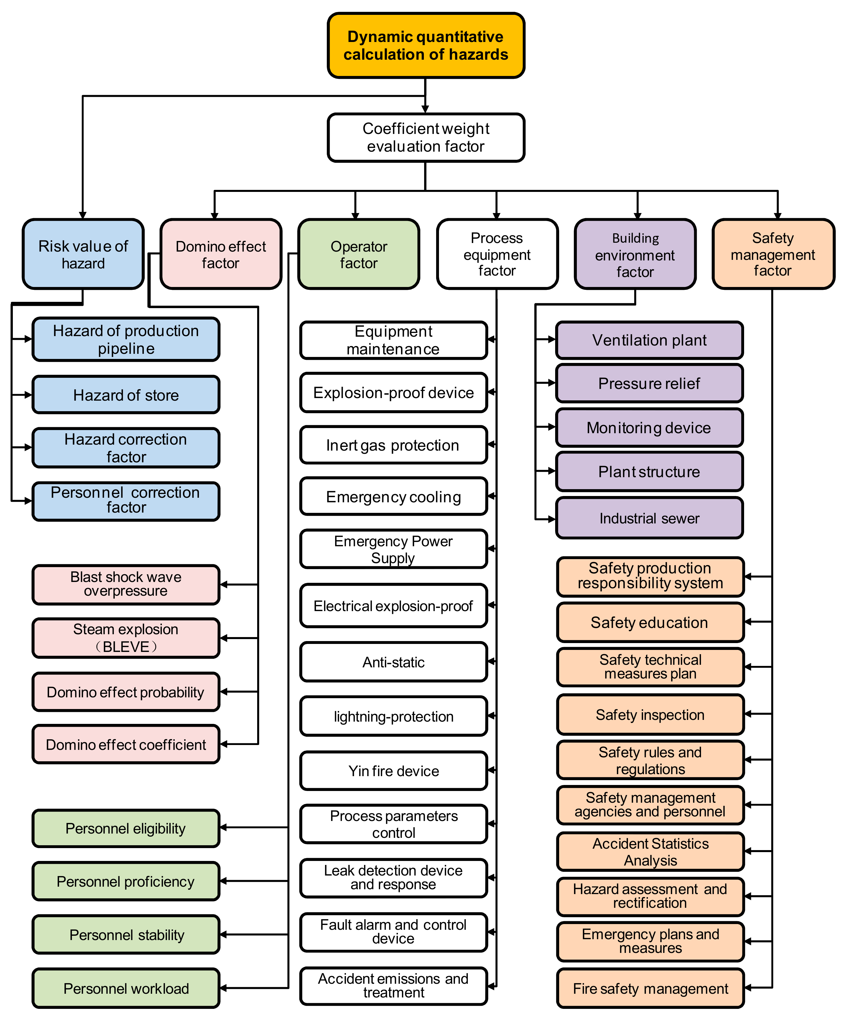
In the dynamic semi-quantitative calculation model for chemical hazards, the six weighting factors are the risk value factor of the hazard, domino effect factor, operator factor, process/equipment factor, building environment factor, and safety management factor. In this article we aimed to study the dynamic quantitative risk values of chemical hazards. The dynamic focus is on all quantitative and semi-quantitative data changes which need to be dynamically monitored, such as real-time changes in the output of hazards in the production pipeline according to the input value of the monitoring point. Therefore, a monitoring point setup matrix was chosen to calculate the overall dynamic quantitative data. The description of the letters used in the equations in this section is shown in

Table 8. Chemical hazard dynamic quantitative calculation model parameters used in the calculation of parameters.

Parameters:
q  Chemical hazards storage mass(ton);
q’  Chemical hazards production site mass (ton);
Q  Chemical hazards storage critical mass (ton);
Q’  Chemical hazards production site critical mass (ton);
i  The ith monitoring point
m  Read m monitoring point data
N  n kinds of chemical substances.
b2  Domino effect probability unit
b3  Domino effect probability
R’  The final optimized risk value

.

3.1. Risk Value Factor of a Hazard, Denoted a (Also R₃)

From the previous analysis, we define the two matrix equations for the variable q in the chemical hazards storage area and the variable q’ in the production site, as shown in Equations (20) and (21).

$$q=\left[\begin{array}{cccccc}{q}_{11}& q_{12}& & \cdots & & q_{1m}\\ q_{21}& q_{22}& & & & q_{2m}\\ & & \ddots & & ⋰& \\ ⋮& & & ⋰& & ⋮\\ & & ⋰& & \ddots & \\ q_{n1}& q_{n2}& & \cdots & & q_{nm}\end{array}\right]$$

(20)

$$q{}^{\prime }=\left[\begin{array}{cccccc}q{{}^{\prime }}_{11}& q{{}^{\prime }}_{12}& & \cdots & & q{{}^{\prime }}_{1m}\\ q{{}^{\prime }}_{21}& q{{}^{\prime }}_{22}& & & & q{{}^{\prime }}_{2m}\\ & & \ddots & & ⋰& \\ ⋮& & & ⋰& & ⋮\\ & & ⋰& & \ddots & \\ q{{}^{\prime }}_{n1}& q{{}^{\prime }}_{n2}& & \cdots & & q{{}^{\prime }}_{nm}\end{array}\right]$$

(21)

When the chemical hazards in the storage area and production pipeline are determined, the correction factor and critical value of the hazard can be found in the table. The correction coefficient is β, the chemical hazards storage critical mass is Q, and the chemical hazards production site critical mass is Q’, so the relative ratios in the available matrices are as shown in Equations (22) and (23).

$$A=\left[\begin{array}{cccccc}\frac{{\beta }_1}{Q_1}& \frac{{\beta }_2}{Q_2}& & \cdots & & \frac{{\beta }_n}{Q_n^{}}\end{array}\right]$$

(22)

$$A{}^{\prime }=\left[\begin{array}{cccccc}\frac{{\beta }_1}{Q{{}^{\prime }}_1}& \frac{{\beta }_2}{Q{{}^{\prime }}_2}& & \cdots & & \frac{{\beta }_n}{Q{{}^{\prime }}_n^{}}\end{array}\right]$$

(23)

According to Equations (2) to (4), we can calculate the risk value factor of hazard a_i as shown in Equation (24).

$$a_i=\alpha \ast (A\ast q_i+A{}^{\prime }\ast q_i{}^{\prime })$$

(24)

Therefore, the value of a is as shown in Equation (25).

$$a=\left[\begin{array}{cccccc}{a}_1& a_2& & \cdots & & a_m\end{array}\right]$$

(25)

3.2. Domino Effect Factor, Denoted b

The parameters q and q’ can be read out from the risk value factors of a hazard, and their sum is a variable that affects the domino effect. The equation of total hazard mass can be obtained from Equations (20) and (21), and it is as shown in Equation (26).

$$q{}^{″}=q+q{}^{\prime }=\left[\begin{array}{cccccc}{q}_{11}+q{{}^{\prime }}_{11}& q_{12}+q{{}^{\prime }}_{12}& & \cdots & & q_{1m}+q{{}^{\prime }}_{1m}\\ q_{21}+q{{}^{\prime }}_{21}& q_{22}+q{{}^{\prime }}_{22}& & & & q_{2m}+q{{}^{\prime }}_{2m}\\ & & \ddots & & ⋰& \\ ⋮& & & ⋰& & ⋮\\ & & ⋰& & \ddots & \\ q_{n1}+q{{}^{\prime }}_{n1}& q_{n2}+q{{}^{\prime }}_{n2}& & \cdots & & q_{nm}+q{{}^{\prime }}_{nm}\end{array}\right]$$

(26)

We do not consider the impacts between various hazards, because the impact of each calculation is too complex to study here in detail. The jth substance of all those where the monitoring point is located, defined as the data of the jth row, can be obtained from Equation (26) and is shown in Equation (27).

$$q_j{}^{″}=q_j+q{{}^{\prime }}_j=\left[\begin{array}{cccccc}{q}_{j1}+q{{}^{\prime }}_{j1}& q_{j2}+q{{}^{\prime }}_{j2}& & \cdots & & q_{jm}+q{{}^{\prime }}_{jm}\end{array}\right]$$

(27)

3.2.1. Overpressure Explosion Model and Vapor Explosion Model Calculation

The specified overpressure explosion model is the Δp data set, the vapor explosion model is the q(r) data set, and b₁ is defined as shown in Equation (28).

$$b_1=\left[\begin{array}{c}\mathsf{\Delta }\mathrm{p}\\ \mathrm{q}\left(\mathrm{r}\right)\end{array}\right]=\left[\begin{array}{cccccc}{\mathsf{\Delta }\mathrm{p}}_1& {\mathsf{\Delta }\mathrm{p}}_2& & \cdots & & {\mathsf{\Delta }\mathrm{p}}_{\mathrm{m}}\\ {\mathrm{q}}_1\left(\mathrm{r}\right)& {\mathrm{q}}_2\left(\mathrm{r}\right)& & \cdots & & {\mathrm{q}}_{\mathrm{m}}\left(\mathrm{r}\right)\end{array}\right]$$

(28)

(1)

Overpressure explosion model

Taking the overpressure explosion model of the ith monitoring point, we can get $\Delta p_{ji}$ from Equations (5) to (7), and (27), as shown in Equation (29).

$$\mathsf{\Delta }{p}_{\mathrm{ji}}=P_0\left\{\frac{0.137}{L^3\left[\frac{P_0}{1.8\alpha {}^{\prime }(q_{ji}+q{{}^{\prime }}_{ji})Q_c}\right]}+\frac{0.119}{L^2{\left[\frac{P_0}{1.8\alpha {}^{\prime }(q_{ji}+q{{}^{\prime }}_{ji})Q_c}\right]}^{\frac{2}{3}}}+\frac{0.269}{L^{}{\left[\frac{P_0}{1.8\alpha {}^{\prime }(q_{ji}+q{{}^{\prime }}_{ji})Q_c}\right]}^{\frac{1}{3}}}-0.019\right\}$$

(29)

We define the overpressure explosion model device container specification matrix as

$$X=\left[\begin{array}{cccc}{x}_1& x_2& x_3& x_4\end{array}\right]=\left[\begin{array}{cccc}\mathrm{Atmospheric} \mathrm{pressure}& \mathrm{Pressure}& \mathrm{Long} \mathrm{type}& \mathrm{Small} \mathrm{type}\end{array}\right]$$

(30)

with restrictions:$x_1,x_2,x_3,x_4\in \left\{0,1\right\},\mathrm{and} x_1+x_2+x_3+x_4=1$, according to the device container, to set the possible condition equations shown in

Table 9. Overpressure model equipment container condition correspondence table.

Number	x Value	Condition	Result
1	x1 = 1	Δp ≥ 22 kpa	b2 = Y=−18.96 + 2.44lnPs
		Δp < 22 kpa	b3 = 0
2	x2 = 1	Δp ≥ 16 kpa	b2 = Y=−42.44 + 4.33lnPs
		Δp < 16 kpa	b3 = 0
3	x3 = 1	Δp ≥ 31 kpa	b2 = Y=−28.07 + 3.16lnPs
		Δp < 31 kpa	b3 = 0
4	x4= 1	Δp ≥ 37 kpa	b2 = Y=−17.79 + 2.18lnPs
		Δp < 37 kpa	b3 = 0

.

(2)

Vapor explosion modell

Taking the vapor explosion model of the ith monitoring point, we can get q_ji(r) and t_i from Equations (8) to (10), and (27), as shown in Equations (31) and (32).

$${\mathrm{q}}_{\mathrm{ji}}\left(\mathrm{r}\right)=\frac{{\mathrm{q}}_0{\left[2.9\ast {\left(q_{ji}+q{{}^{\prime }}_{ji}\right)}^{1/3}\right]}^2\mathrm{r}\left(1-0.058\mathrm{lnr}\right)}{{\left\{{\left[2.9\ast {\left(q_{ji}+q{{}^{\prime }}_{ji}\right)}^{1/3}\right]}^2+r^2\right\}}^{3/2}}$$

(31)

$$t_{\mathrm{j}i}=0.45\ast {\left(q_{ji}+q{{}^{\prime }}_{ji}\right)}^{1/3}$$

(32)

We define the vapor explosion model device container specification matrix as shown in Equation (33).

$$Y=\left[\begin{array}{cc}{y}_1& y_2\end{array}\right]=\left[\begin{array}{cc}\mathrm{Atmospheric} \mathrm{pressure}& \mathrm{Pressure}\end{array}\right]$$

(33)

With restrictions $y_1,y_2\in \left\{0,1\right\},\mathrm{and} y_1+y_2=1$, according to the device container, to set the possible condition equations in

Table 10. Steam model equipment container condition correspondence table.

Number	y Value	Condition	Result
1	y1 = 1	qji(r) ≥ 15 kpa and t ≥ 10 min	b2 = Y = 12.54 − 1.847(−1.128lnI − 2.667 × 10−5V + 9.877)
		qji(r) < 15 kpa or t < 10 min	b3 = 0
2	y2 = 1	qji(r) ≥ 50 kpa and t ≥ 10 min	b2 = Y = 12.54−1.847(−0.947lnI + 8.835V0.032)
		qji(r) < 50 kpa or t < 10 min	b3 = 0

.

3.2.2. Overpressure Explosion and Vapor Explosion Model Probability Calculations

We define the overpressure explosion probability as the b_3i data set and the vapor explosion probability as the b’_3i data set; the explosion probability matrix can then be constructed as shown in Equations (34) to (36).

$$b_3=\left[\begin{array}{cccccc}{\mathrm{b}}_3{}_1& {\mathrm{b}}_3{}_2& & \cdots & & {\mathrm{b}}_3{}_{\mathrm{m}}\\ {{\mathrm{b}}^{\prime }}_3{}_1& {{\mathrm{b}}^{\prime }}_3{}_2& & \cdots & & {{\mathrm{b}}^{\prime }}_3{}_{\mathrm{m}}\end{array}\right]$$

(34)

$$b_{3i}=\frac{1}{\sqrt{2\pi }}{\displaystyle {\int }_{-\infty }^{b_{2i}-5}{e}^{-x^2/2}dx}$$

(35)

$$b{{}^{\prime }}_{3i}=\frac{1}{\sqrt{2\pi }}{\displaystyle {\int }_{-\infty }^{b{{}^{\prime }}_{2i}-5}{e}^{-x^2/2}dx}$$

(36)

3.2.3. Domino Effect Coefficient

Because the multilayer domino effect is complicated, but the calculation method is the same, we only consider the domino effect for a single layer. According to Equation (12), the domino effect coefficient is as shown in Equation (37).

$$b_{4i}=(1+b_{3i})(1+b{{}^{\prime }}_{3i})$$

(37)

The output domino effect coefficient b is as shown in Equation (38).

$$b=\left[\begin{array}{cccccc}{b}_{41}& b_{42}& & \cdots & & b_{4m}\end{array}\right]$$

(38)

3.3. Operator Factor, Denoted c

In the calculation of the operator’s index coefficient, there are five items involved in the calculation of important information: the post (g), certificate (t₁), working age (t₂), accident-free time (t₃), and working time (t₄).We set the input matrix as shown in Equation (39).

$$C_i=\left[\begin{array}{c}{\mathrm{Name}}_{} 1\\ {\mathrm{Name}}_{} 2\\ \\ ⋮\\ \\ {\mathrm{Name}}_{} \mathrm{n}\end{array}\right]={\left[\begin{array}{ccccc}{\mathrm{g}}_1& t_{11}& t_{21}& t_{31}& t_{41}\\ {\mathrm{g}}_2& t_{12}& t_{22}& t_{32}& t_{42}\\ & & & & \\ ⋮& ⋮& ⋮& ⋮& ⋮\\ & & & & \\ {\mathrm{g}}_{\mathrm{n}}& t_{1n}& t_{2n}& t_{3n}& t_{4n}\end{array}\right]}_i$$

(39)

This article uses real-time quantitative data, so there is no situation of different people in the same location; that is, N = 1 and M₀ = N₀.When g_k = g_j (k ≠ j, k = 1,2,…,n, j = 1,2,…,n), from Equations (13)–(15), H_pi is as shown in Equation (40).

$$H_{p\mathrm{i}}={\displaystyle \prod _{j=1}^n\left\{\left[1-\frac{1}{k_2\left(\frac{t_2}{T_2}+1\right)}\right]\ast \left[1-\frac{1}{k_3\left({\left(\frac{t_3}{T_3}\right)}^2+1\right)}\right]\ast \left[1-k_4{\left(\frac{t_4}{T_4}-1\right)}^2\right]\right\}}$$

(40)

The elements u in the set {g₁,g₂,…,g_n}_i can make up H_p, so the operator risk is as shown in Equation (41).

$$H_u{}_{\mathrm{i}}=1-\underset{j=1}{\overset{m}{\Pi }}\left(1-H_{pj}\right)$$

(41)

From the calculation process, it can be seen that H_u has a maximum close to 1. Taking into account the limited impact of personnel factors, when the value is 0.8, the coefficient c is specified as 1. The worse the indicator, the greater the coefficient c. The highest value of H_u is 1 and the lowest value is specified as 0.6, so when the value is lower than 0.6, it is calculated using 0.6 instead. Therefore, the range of c values is 0.8 to 1.33.

When H_ui ≤ 0.6, we let H_ui = 0.6, and c_i is calculated as shown in Equation (42).

$$c_{\mathrm{i}}=\frac{0.8}{H_{\mathrm{u}}{}_{\mathrm{i}}}$$

(42)

The coefficient c is as shown in Equation (43).

$$c=\left[\begin{array}{cccccc}{c}_1& c_2& & \cdots & & c_{\mathrm{m}}\end{array}\right]$$

(43)

3.4. Process/Equipment Factor, Denoted d

The process/equipment index factor includes a total of 13 second-level factors, namely, equipment maintenance, explosion-proof devices, inert gas protection, emergency cooling, emergency power supply, electrical explosion-proofing, anti-static, lightning protection, devices for preventing fire, process parameter control, leak detection device and response, fault alarm and control devices, and accidental discharge and treatment. There is a certain number of third-level index factors for each second-level index factor, and the scores for each third-level index factor are not the same. There are two kinds of calculation logic, “and” and “or”, for the third-level indices, with the highest total score being 310 points. Coefficient d is defined as 1 at 248 points (80%), and the worse the indicator, the greater the coefficient d. The highest is 310 points, and when the value is less than 186 points (60%), it is calculated using 186 points. Therefore, the range of d values is 0.8 to 1.33.

According to Table 5, the score matrix

D = [8 6 24 11 13 15 10 12 12 7 7 7 12 11 11 15 11 11 10 13 10 11 13 13 14 11]

can be built for input data X_i, where

X_i = [X₁₁ X₁₂ X₂₁ X₂₂ X₃₁ X₃₂ X₄₁ X₄₂ X₅ X₆ X₇ X₈ X₉ X_A X_B1 X_B2 X_C1 X_C2 X_C3 X_C4 X_C5 X_D1 X_D2 X_D3 X_D4 X_D5]^T

with restrictions as follows:

(1)

The original input data are only 0 or 1, that is, X₁₁, X₁₂, …, X_D5 ∈ {0,1};

(2)

X₁₁ + X₁₂ ≤ 1;

(3)

X₃₁ + X₃₂ ≤ 1;

(4)

X₄₁ + X₄₂ ≤ 1;

(5)

X₅ = X₅₁ + X₅₂ ≤ 1;

(6)

X₆ = X₆₁ + X₆₂ + X₆₃ + X₆₄ + X₆₅ + X₆₆ + X₆₇ + X₆₈ + X₆₉ ≤ 1;

(7)

X₇ = X₇₁ + X₇₂ + X₇₃ + X₇₄ + X₇₅ ≤ 1;

(8)

X₈ = X₈₁ + X₈₂ + X₈₃ + X₈₄ + X₈₅;

(9)

X₉ = X₉₁ + X₉₂ + X₉₃;

(10)

X_A = X_A1 + X_A2 + X_A3 ≤ 1;

(11)

X_B1 + X_B2 ≤ 1.

According to the above score matrix, input data, and restrictions, we can get x_i, where x_i is the multiplication of matrix D and matrix X_i, as shown in Equation (44).

x_i = DX_i

(44)

when x_i ≥ 186, the definition of value d is as shown in Equation (45).

$$d_i=\frac{248}{x_i}$$

(45)

when x_i < 186, the definition of value d is $d_i=1.33$.

The process/equipment index coefficient d is as shown in Equation (46).

$$d=\left[\begin{array}{cccccc}{d}_1& d_2& & \cdots & & d_m\end{array}\right]$$

(46)

3.5. Building Environmental Factor, Denoted e

The building environmental index factor includes a total of five second-level factors, namely, ventilation plant, pressure relief, monitoring device, plant structure, and industrial sewer. There are a certain number of third-level index factors for each second-level index factor, and the third-level index factor scores are not the same. There are two kinds of calculation logic, “and” and “or”, for the third-level indices, with the highest total score being 89 points. Coefficient e is defined as 1at 71 points (80%), and the worse the indicator, the greater the coefficient e. The highest is 89 points, and when the value is less than 53 points (60%), it is calculated using 53 points. Therefore, the range of e values is 0.8 to 1.33.

According to Table 4, the score matrix

E = [6 8 8 8 10 12 18 5 5 5 5 5 5 5]

can be built with input data Y_i such that Y_i= [Y₁₁ Y₂₁ Y₂₂ Y₂₃ Y₃₁ Y₃₂ Y₃₃ Y₄₁ Y₄₂ Y₄₃ Y₄₄ Y₄₅ Y₅₁ Y₅₂]^T and with restrictions as follows:

(1)

The original input data are only 0 or 1, that is, Y₁₁, Y₂₁,…, Y₅₂ ∈ {0,1};

(2)

Y₂₁ + Y₂₂ + Y₂₃ ≤ 1.

According to the above score matrix, input data, and restrictions, we can get y_i where y_i is the multiplication of matrix E and matrix Y_i, as shown in Equation (47).

y_i = EY_i

(47)

when y_i ≥ 53, the definition of e is as shown in Equation (48).

$$e_i=\frac{71}{{\mathrm{y}}_i}$$

(48)

when y_i < 53, the definition of e is $e_i=1.33$.

The construction environmental index coefficient e is as shown in Equation (49).

$$e=\left[\begin{array}{cccccc}{e}_1& e_2& & \cdots & & e_m\end{array}\right]$$

(49)

3.6. Safety Management Factor, Denoted f

The safety management index factor includes a total of 10 s-level factors, namely, safety production responsibility system, safety education, safety technical measures plan, safety inspection, safety rules and regulations, safety management agencies and personnel, statistical analysis of accidents, hazard assessment and rectification, contingency plans and measures, and fire safety management. There are a certain number of third-level index factors for each second-level index factor, and the third-level index factor scores are not the same. The total score is 100 points. At 80 points, coefficient f is defined as 1, and the worse the indicator, the greater the coefficient f. The highest is 100 points, and when the value is less than 60 points, it is calculated using 60 points. Therefore, the range of f values is 0.8 to 1.33.

According to Table 5, score matrix

F = [1.1 1.25 2.50 1.43 0.77 2.00 3.30 2.50 1.11 1.00]

can be built for input data Z_i, where Z_i= [Z₁ Z₂ Z₃ Z₄ Z₅ Z₆ Z₇ Z₈ Z₉ Z_A]^T, with restrictions as follows:

(1)

The original input data are only 0 or 1, that is, Z₁₁, Z₁₂,…, Z_AA ∈ {0,1};

(2)

Z₁ = Z₁₁ + Z₁₂ + Z₁₃ + Z₁₄ + Z₁₅ + Z₁₆ + Z₁₇ + Z₁₈ + Z₁₉;

(3)

Z₂ = Z₂₁ + Z₂₂ + Z₂₃ + Z₂₄ + Z₂₅ + Z₂₆ + Z₂₇ + Z₂₈;

(4)

Z₃ = Z₃₁ + Z₃₂ + Z₃₃ + Z₃₄;

(5)

Z₄ = Z₄₁ + Z₄₂ + Z₄₃ + Z₄₄ + Z₄₅ + Z₄₆ + Z₄₇;

(6)

Z₅ = Z₅₁ + Z₅₂ + Z₅₃ + Z₅₄ + Z₅₅ + Z₅₆ + Z₅₇ + Z₅₈ + Z₅₉ + Z_5A + Z_5B + Z_5C + Z_5D;

(7)

Z₆ = Z₆₁ + Z₆₂ + Z₆₃ + Z₆₄ + Z₆₅;

(8)

Z₇ = Z₇₁ + Z₇₂ + Z₇₃;

(9)

Z₈ = Z₈₁ + Z₈₂ + Z₈₃ + Z₈₄ + Z₈₅ + Z₈₆ + Z₈₇ + Z₈₈ + Z₈₉;

(10)

Z₉ = Z₉₁ + Z₉₂ + Z₉₃ + Z₉₄ + Z₉₅ + Z₉₆ + Z₉₇ + Z₉₈ + Z₉₉;

(11)

Z_A = Z_A1 + Z_A2 + Z_A3 + Z_A4 + Z_A5 + Z_A6 + Z_A7 + Z_A8 + Z_A9 +Z_AA.

According to the above score matrix, input data, and restrictions, we can get z_i, where z_i is the multiplication of matrix F and matrix Z_i as shown in Equation (50).

z_i = FZ_i

(50)

when z_i ≥ 60, the definition of f is as shown in Equation (51).

$$f_i=\frac{80}{z_i}$$

(51)

when z_i < 60, the definition of f is $f_i=1.33$.

The safety management index coefficient f is as shown in Equation (52).

$$f=\left[\begin{array}{cccccc}{f}_1& f_2& & \cdots & & f_m\end{array}\right]$$

(52)

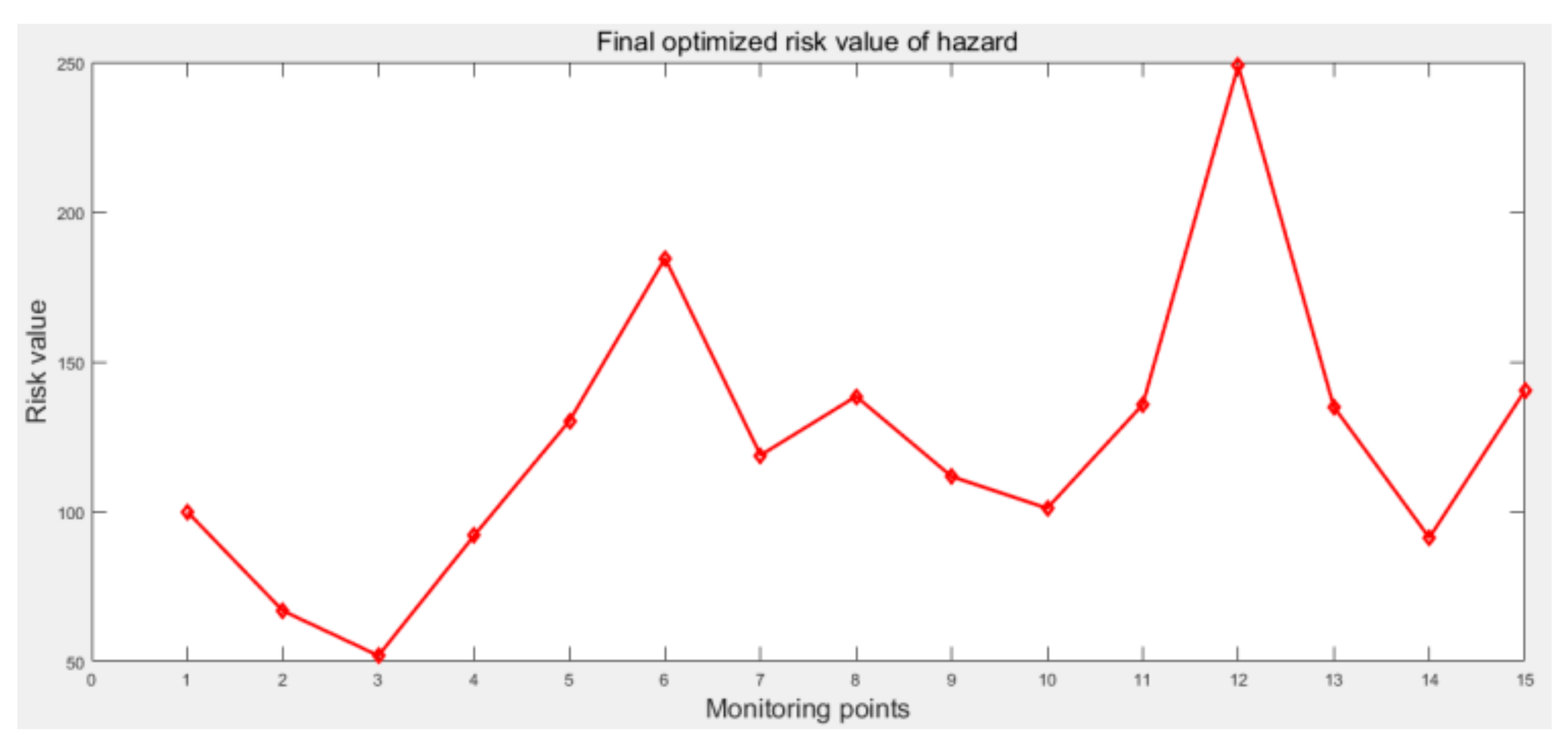
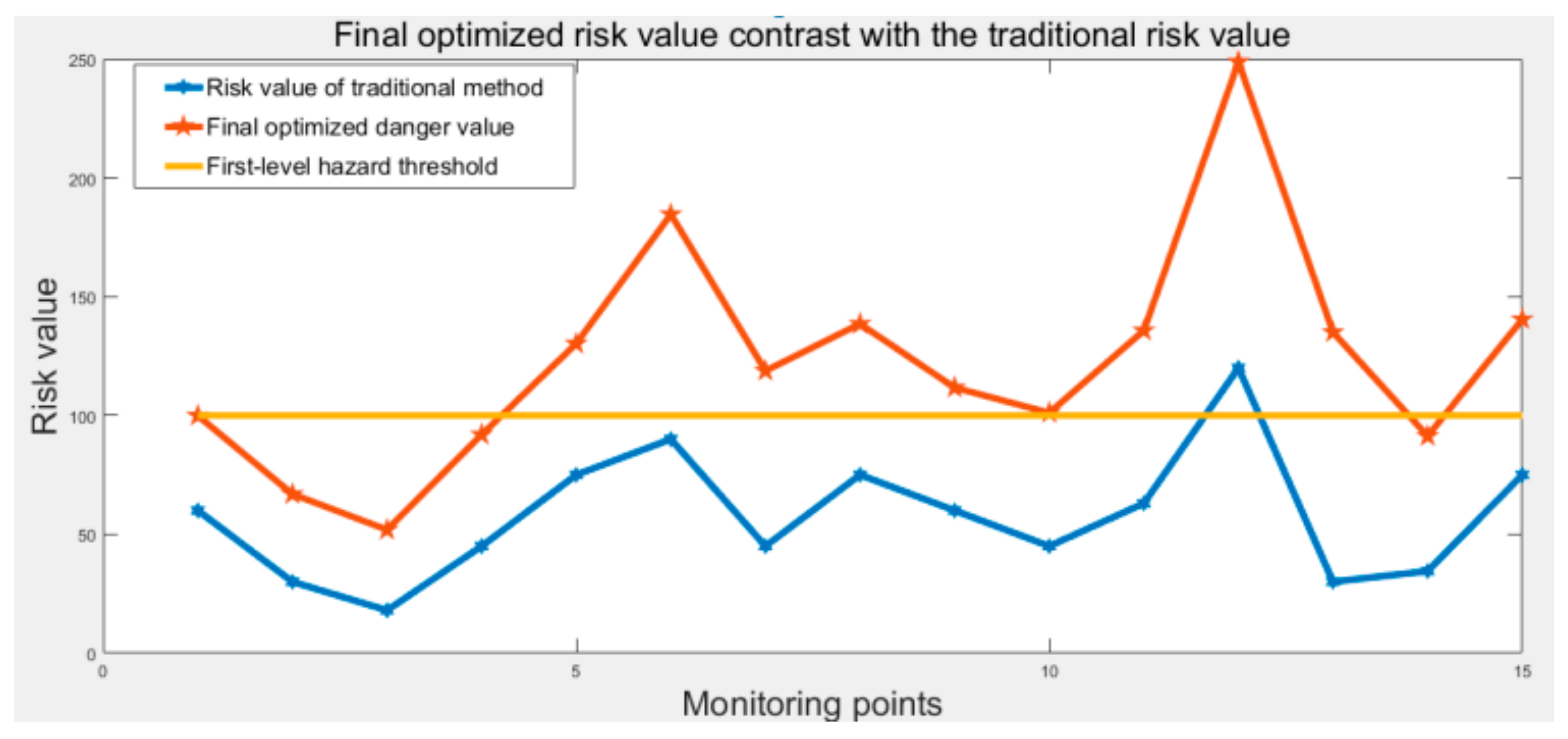
3.7. Calculation Results

We used forced pair comparison (

Table 11. Pairwise comparison to determine the weight of each factor.

Evaluation Items	One-to-One Comparison Result										Points Accumulated	Weight (ωj)
Domino effect	1	1	1	1							4	0.4
Operator	0				1	1	0				2	0.2
Process/equipment		0			0			1	0		1	0.1
Building environment			0			0		0		1	1	0.1
Safety management				0			1		1	0	2	0.2
Total											10	1.0

) to calculate the final optimized risk value R’ of the hazards. R’ is as shown in Equation (53):

$$R_{\mathrm{i}}{}^{\prime }=R_{3\mathrm{i}}\ast {\displaystyle \sum _{\mathrm{j}=1}^5{\omega }_{\mathrm{j}}{\mathrm{K}}_{\mathrm{i}}(\mathrm{j})}$$

(53)

where ${\mathrm{K}}_{\mathrm{i}}(\mathrm{j})$ is a five-point indicator function of i monitoring points.

4. Case Analysis

4.1. Major Hazards Factory Fact Sheet

At present, there are a total of 64 chemical plants in the particular chemical industry park we are studying; each chemical plant in it has its own characteristics. This chemical industrial park is potentially high-risk, and the chemical plants in the park are concentrated, and there are many major hazards such as inflammable, explosive and toxic. Applying our dynamic semi-quantitative model, chemical park managers can understand and grasp the risk values and risk trends of each chemical plant in the park, and further grasp the risk level of each chemical plant. For these chemical plants where the first-level risk or risk trend is bad, the chemical park managers should focus on monitoring and management, and notify the corresponding chemical plant to improve so as to reduce risks. One of the chemical plants is a high-yield one in this chemical industrial park, and a co-author of this article is an employee of the chemical plant who was able to provide accurate data for calculations, so this chemical plant was chosen as a calculation case. The chemical plant has a spherical tank area which has two spherical tanks that are pressure vessels filled with methanol and ethanol, respectively. The hazard masses are subject to real-time monitoring. We chose 15 monitoring points, that is, m=15, in the monitoring data and calculated the variable q in storage and the variable q’ in the production pipeline as follows (unit: ton). In the two rows of the matrices in the follow-up case, the one above is methanol and that below is ethanol, as shown in Equations (54) to (56).

$$q~q{}^{\prime }~\left[\begin{array}{c}\mathrm{Methanol} \\ \mathrm{Ethanol}\end{array}\right]$$

(54)

The variables q and q’ were therefore calculated as shown in Equations (55) and (56).

$$q=\left[\begin{array}{ccccccccccccccc}200& 70& 80& 180& 250& 200& 150& 350& 180& 120& 210& 300& 50& 80& 260\\ 200& 130& 40& 120& 250& 400& 150& 150& 220& 180& 210& 500& 150& 150& 240\end{array}\right]$$

(55)

$$q{}^{\prime }=\left[\begin{array}{ccccccccccccccc}3& 6& 4& 6& 0& 0& 8& 5& 7& 8& 10& 14& 10& 8& 4\\ 7& 6& 8& 6& 10& 20& 12& 10& 8& 10& 9& 16& 30& 12& 15\end{array}\right]$$

(56)

The resident population within 500 m of the hazards is 302, and the distance to a surrounding hazard is 70 m (the distance to other hazards is over 500 m, giving no possible impact). The names, post, certificate, working age, accident-free time, and working time of operators on the 15 monitoring points are shown in

Table 12. Information on operators at the monitoring points.

Monitoring Point	Name	Post	Certificate	Working Age (Years)	Accident-Free Time (Years)	Working Time (Hours/Day)
1	Tom	Storage	Yes	1	1	8
2	Tom	Storage	Yes	1	1	9
3	Tom	Storage	Yes	1	1	10
4	Tom	Storage	Yes	1	1	8
5	Tom	Storage	Yes	2	2	8
6	Tom	Storage	Yes	2	0	8
7	Tom	Storage	Yes	2	0	10
8	Tom	Storage	Yes	2	1	8
9	Jack	Storage	Yes	5	5	8
10	Jack	Storage	Yes	5	5	10
11	Mark	Storage	Yes	2	0	8
12	Mark	Storage	Yes	2	0	8
13	Mark	Storage	Yes	2	0	8
14	Jose	Storage	Yes	1	1	8
15	Joe	Storage	Yes	4	4	10

.

4.2. Dynamic Quantitative Calculation of Hazards

4.2.1. Risk Value Factor of Hazards, Denoted a

As the hazards are methanol and ethanol, we can look up the table to obtain $\alpha =2$; the resulting A and A′ are shown in Equation (57).

$$A=\left[\begin{array}{cc}\frac{1.5}{20}& \frac{1.5}{20}\end{array}\right]\mathrm{and} A{}^{\prime }=\left[\begin{array}{cc}\frac{1.5}{2}& \frac{1.5}{2}\end{array}\right]$$

(57)

The value of a can be obtained from $a_i=\alpha \ast (A\ast q_i+A{}^{\prime }\ast q_i{}^{\prime })$ and $a=\left[\begin{array}{cccccc}{a}_1& a_2& & \cdots & & a_m\end{array}\right]$, as shown in Equation (58).

$$a=\left[\begin{array}{ccccccccccccccc}75& 48& 36& 63& 90& 120& 75& 97.5& 82.5& 72& 91.5& 165& 90& 64.5& 103.5\end{array}\right]$$

(58)

4.2.2. Domino Effect Factor, Denoted b

From the risk value factor of hazards (previous section), we know that the parameters q and q’ are large variables that affect the domino effect. The total hazards calculation can then be obtained from Equations (26) and (27), as shown in Equation (59) (unit: ton).

$$q{}^{″}=\left[\begin{array}{ccccccccccccccc}203& 76& 84& 186& 250& 200& 158& 355& 187& 128& 220& 314& 60& 88& 264\\ 207& 136& 48& 126& 260& 420& 162& 160& 228& 190& 219& 516& 180& 162& 255\end{array}\right]$$

(59)

(1)

Overpressure explosion

From the look-up table, α’ = 0.04, methanol’s heat of combustion Q_c = 22,675 kJ/kg, ethanol’s heat of combustion Q_c = 29,640 kJ/kg, p₀ = 101,325 pa, and L = 70 m is given in the example; from Equation (29), $\Delta p$ can be obtained as shown in Equation (60).

$$\Delta p=\left[\begin{array}{ccccccccccccccc}243& 118& 126& 227& 285& 240& 200& 378& 228& 171& 258& 342& 100& 130& 298\\ 304& 219& 103& 207& 365& 542& 251& 248& 328& 284& 318& 645& 272& 251& 359\end{array}\right]$$

(60)

Since it is a pressure vessel, b₂ can be obtained according to Equation (30) and Table 9, and it is as shown in Equation (61).

$$b_2=\left[\begin{array}{ccccccccccccccc}11.2& 8.1& 8.4& 11.0& 12.0& 11.2& 10.4& 13.2& 11.0& 9.7& 11.5& 12.7& 7.4& 8.6& 12.1\\ 12.2& 10.8& 7.5& 10.6& 13.0& 14.7& 11.4& 11.3& 12.6& 11.9& 12.4& 15.5& 11.7& 11.4& 12.9\end{array}\right]$$

(61)

Therefore, according to Equation (35), the probability of overpressure explosion is as shown in Equation (62).

$$b_{3c}=\left[\begin{array}{ccccccccccccccc}1& 1& 1& 1& 1& 1& 1& 1& 1& 1& 1& 1& 1& 1& 1\\ 1& 1& 1& 1& 1& 1& 1& 1& 1& 1& 1& 1& 1& 1& 1\end{array}\right]$$

(62)

(2)

Vapor explosion

From the look-up table, q₀ = 200 kw/m², and L = 70 m is given in the example, so q(r) and t can be obtained from Equations (31) and(32) as shown in Equations(63) and (64).

$$q(r)=\left[\begin{array}{ccccccccccccccc}49& 56& 56& 49& 47& 49& 51& 43& 49& 53& 48& 45& 57& 56& 46\\ 49& 53& 58& 53& 47& 42& 51& 51& 48& 50& 48& 40& 50& 51& 47\end{array}\right]$$

(63)

$$\mathrm{t}=\left[\begin{array}{ccccccccccccccc}26& 19& 20& 26& 28& 26& 24& 32& 26& 23& 27& 31& 18& 20& 29\\ 27& 23& 16& 23& 29& 34& 25& 25& 27& 26& 27& 36& 25& 25& 29\end{array}\right]$$

(64)

Since it is a pressure vessel, we claim q(r) ≥ 50 kpa and t ≥ 600 s (10 min). It can be seen from the above equation that t is less than 600 s, so they do not all produce the domino effect of a vapor explosion; thus, the probability of vapor explosion is 0, as shown in Equation (65).

$$b{{}^{\prime }}_{3c}=\left[\begin{array}{ccccccccccccccc}0& 0& 0& 0& 0& 0& 0& 0& 0& 0& 0& 0& 0& 0& 0\\ 0& 0& 0& 0& 0& 0& 0& 0& 0& 0& 0& 0& 0& 0& 0\end{array}\right]$$

(65)

(3)

Domino effect coefficient

Methanol and ethanol produce the same domino effect, so we only need to take one set of data; from Equation (38), the domino effect coefficient b is as shown in Equation (66).

$$b=\left[\begin{array}{ccccccccccccccc}2& 2& 2& 2& 2& 2& 2& 2& 2& 2& 2& 2& 2& 2& 2\end{array}\right]$$

(66)

4.2.3. Operator Factor, Denoted c

From the input monitoring point operator post information in Table 12 and Equation (40), H_p can be obtained as shown in Equation (67).

$${\mathrm{H}}_{\mathrm{p}}=\left[\begin{array}{ccccccccccccccc}0.83& 0.81& 0.77& 0.83& 0.92& 0.48& 0.45& 0.86& 0.97& 0.91& 0.48& 0.48& 0.48& 0.83& 0.90\end{array}\right]$$

(67)

According to H_p and Equation (41), H_u can be obtained as shown in Equation (68).

$${\mathrm{H}}_{\mathrm{u}}=\left[\begin{array}{ccccccccccccccc}0.83& 0.81& 0.77& 0.83& 0.92& 0.48& 0.45& 0.86& 0.97& 0.91& 0.48& 0.48& 0.48& 0.83& 0.90\end{array}\right]$$

(68)

when H_ui ≤ 0.6, we let H_ui = 0.6; the H’_u values obtained after adjustment are as shown in Equation (69).

$${{\mathrm{H}}^{\prime }}_{\mathrm{u}}=\left[\begin{array}{ccccccccccccccc}0.83& 0.81& 0.77& 0.83& 0.92& 0.60& 0.86& 0.97& 0.91& 0.60& 0.60& 0.60& 0.60& 0.83& 0.90\end{array}\right]$$

(69)

By Equation (42), the available operator factor coefficient c is as shown in Equation (70).

$$\mathrm{c}=\left[\begin{array}{ccccccccccccccc}0.97& 0.99& 1.03& 0.97& 0.87& 1.33& 1.33& 0.94& 0.82& 0.88& 1.33& 1.33& 1.33& 0.97& 0.88\end{array}\right]$$

(70)

4.2.4. Process/Equipment Factor, Denoted d

From the input data X_i, a preliminary summary of available data is given in

Table 13. Summary of input information for calculation of the process/equipment index.

Xi	Monitoring Points
	1	2	3	4	5	6	7	8	9	10	11	12	13	14	15
X11	1	0	1	0	1	1	0	0	1	1	0	0	0	0	0
X12	0	0	0	1	0	0	1	1	0	0	0	0	1	1	1
X21	1	1	0	0	1	1	1	0	0	1	0	1	0	1	1
X22	1	1	0	1	1	1	1	0	0	1	1	0	1	0	1
X31	1	0	0	1	0	1	1	0	0	0	0	1	0	1	0
X32	0	1	1	0	1	0	0	0	1	0	0	0	1	0	1
X41	1	0	0	1	1	1	0	0	0	0	1	0	1	1	1
X42	0	1	0	0	0	0	0	0	1	1	0	0	0	0	0
X5	1	0	0	1	1	1	1	1	1	1	0	0	1	1	1
X6	1	0	1	1	1	0	1	0	1	0	1	1	1	0	0
X7	1	0	0	1	1	1	0	0	1	1	0	0	1	1	1
X8	2	3	5	4	1	3	4	5	2	3	5	5	2	4	3
X9	3	2	1	1	2	2	2	2	3	3	3	2	2	1	1
XA	1	0	1	1	1	0	0	1	1	1	1	0	0	0	0
XB1	1	1	0	0	0	0	1	1	1	1	0	1	0	1	1
XB2	0	0	1	1	1	0	0	0	0	0	1	0	0	0	0
XC1	1	1	1	0	1	1	1	1	1	1	1	1	0	1	0
XC2	0	1	1	1	0	1	1	1	1	0	1	0	0	0	0
XC3	0	1	1	1	0	0	1	1	1	1	1	1	0	0	0
XC4	1	1	1	1	0	0	0	1	0	0	0	1	1	0	1
XC5	1	1	1	1	1	1	0	0	0	0	0	1	1	0	1
XD1	1	1	1	1	1	1	0	0	0	0	0	1	1	0	1
XD2	1	1	1	0	1	1	1	0	1	0	1	1	1	0	1
XD3	0	1	1	0	1	1	1	0	0	1	1	1	1	0	1
XD4	0	1	1	0	0	0	1	1	1	1	1	1	1	0	1
XD5	1	1	0	0	1	0	0	1	0	1	1	1	0	0	1

.

From x_i=DX_i, x_i can be obtained as shown in Equation (71).

$$x=\left[\begin{array}{ccccccccccccccc}278& 235& 209& 187& 220& 199& 208& 169& 192& 212& 208& 220& 180& 134& 214\end{array}\right]$$

(71)

According to the value of x, we can further calculate d as shown in Equation (72).

$$\mathrm{d}=\left[\begin{array}{ccccccccccccccc}0.89& 1.06& 1.19& 1.33& 1.13& 1.25& 1.19& 1.33& 1.29& 1.17& 1.19& 1.13& 1.33& 1.33& 1.16\end{array}\right]$$

(72)

4.2.5. Building Environmental Factor, Denoted e

From the input data Y_i, a preliminary summary of available data is given in

Table 14. Summary of input information for calculation of the building environmental index.

Yi	Monitoring Points
	1	2	3	4	5	6	7	8	9	10	11	12	13	14	15
Y11	1	0	1	0	1	1	0	1	1	1	0	0	0	0	1
Y21	1	0	0	0	0	0	1	0	0	1	0	1	0	1	1
Y22	0	1	0	1	1	1	0	0	0	0	1	0	1	0	0
Y23	0	0	0	0	0	0	0	1	1	0	0	0	0	0	1
Y31	1	1	0	1	0	1	1	1	1	0	1	1	0	1	0
Y32	1	1	1	0	1	0	1	0	1	0	0	0	1	0	1
Y33	1	1	1	1	0	1	0	1	1	1	1	1	1	1	1
Y41	1	0	0	1	1	1	0	0	0	0	1	0	1	1	1
Y42	0	1	0	0	0	0	0	0	1	1	0	1	0	0	0
Y43	1	0	0	1	1	1	1	1	1	1	0	0	1	1	1
Y44	1	0	1	1	1	0	1	0	1	0	1	1	1	0	0
Y45	1	0	0	1	1	1	0	1	1	1	1	0	1	1	1
Y51	1	1	1	0	0	0	1	1	1	1	1	0	0	1	1
Y52	1	1	1	1	0	0	0	1	1	0	1	0	1	1	1

.

From y_i = DY_i, we can calculate y, and it is as shown in Equation (73).

$$\mathrm{y}=\left[\begin{array}{ccccccccccccccc}84& 63& 51& 61& 46& 57& 45& 62& 84& 52& 61& 46& 63& 61& 77\end{array}\right]$$

(73)

According to the value of y, we can further calculate e as shown in Equation (74).

$$\mathrm{e}=\left[\begin{array}{ccccccccccccccc}0.85& 1.13& 1.33& 1.16& 1.33& 1.25& 1.33& 1.15& 0.85& 1.33& 1.16& 1.33& 1.13& 1.16& 0.92\end{array}\right]$$

(74)

4.2.6. Safety Management Factor, Denoted f

From the input data Z_i, a preliminary summary of available data is given in

Table 15. Summary of input information for calculation of the safety management index.

Zi	Monitoring Points
	1	2	3	4	5	6	7	8	9	10	11	12	13	14	15
Z1	10	10	10	7.7	6.6	10	3	10	8.8	7.7	10	8.8	7.7	10	10
Z2	10	8.8	8.8	7.5	7.5	8.8	8.8	7.5	7.5	10	10	10	7.5	7.5	10
Z3	10	7.5	7.5	5.0	5.0	5.0	7.5	10	10	10	7.5	7.5	10	10	7.5
Z4	10	8.6	8.6	7.1	7.1	5.7	7.1	7.1	8.6	8.6	8.6	10	10	10	8.6
Z5	10	9.2	9.2	8.5	8.5	6.9	6.9	10	10	10	6.9	6.9	8.5	9.2	10
Z6	10	8.0	10	10	8.0	6.0	8.0	6.0	10	10	10	6.0	6.0	10	8.0
Z7	10	10	6.6	6.6	6.6	6.6	3.3	10	10	10	10	6.6	6.6	10	10
Z8	10	10	7.5	5.0	5.0	5.0	2.5	7.5	7.5	7.5	10	10	10	10	10
Z9	10	10	10	6.6	7.7	8.8	5.5	10	10	8.8	7.7	7.7	8.8	6.6	10
ZA	8	9.0	9.0	10	8.0	9.0	5.0	9.0	9.0	7.0	7.0	8.0	10	10	9.0

.

From z_i = FZ_i, we can calculate z as shown in Equation (75).

$$\mathrm{z}=\left[\begin{array}{ccccccccccccccc}98& 91& 87& 74& 70& 72& 58& 87& 91& 90& 88& 82& 85& 93& 93\end{array}\right]$$

(75)

According to the value of z, we can further calculate f as shown in Equation (76).

$$f=\left[\begin{array}{ccccccccccccccc}0.82& 0.88& 0.92& 1.08& 1.14& 1.11& 1.33& 0.92& 0.88& 0.89& 0.91& 0.98& 0.94& 0.86& 0.86\end{array}\right]$$

(76)

4.3. The Final Optimized Hazard Risk Value

According to Equation (53), we can get R’; the specific values of R’ are shown in Equation (77), and the data trend of R’ is shown in Figure 4.

$$\mathrm{R}{}^{\prime }=\left[\begin{array}{ccccccccccccccc}99.9& 66.9& 51.9& 91.9& 130.2& 184.6& 118.8& 138.5& 111.7& 101.1& 135.7& 248.8& 135.0& 91.3& 140.4\end{array}\right]$$

(77)

4.4. Comparison WITH the Traditional Method of Calculating Hazard Risk Values

The traditional R value can be calculated using Equation (1), as shown in Equation (78).

$$\mathrm{R}=\left[\begin{array}{ccccccccccccccc}60& 30& 18& 45& 75& 90& 45& 75& 60& 45& 63& 120& 30& 34.5& 75\end{array}\right]$$

(78)

The risk value comparison results are shown in Figure 5. According to the data in Figure 5, the traditional R value only considers the hazard of the storage area in the chemical plant, and the risk value is thus relatively low. Only one point out of the 15 monitored time points exceeds the first level of the danger standard value of 100. The final optimized hazard risk value was calculated from data from hazards in the storage area, hazards in the processing pipelines, the domino effect, operators, process/equipment, the building environment, and safety management. Out of the 15 monitoring points in time, 10 points exceeded the first level of the danger standard value of 100, and it is obvious that the optimized risk value has a more realistic result. Using the optimized hazard risk value as an indicator of the overall risk assessment in chemical plants, the real-time data of the six influencing factors can be obtained separately, which can greatly help in the safety analysis of chemical plants. For example, when R’ ≥ 100, the chemical plant is a first-level risk and needs to be heavily regulated. The chemical industry park managers can monitor the risk value fluctuations of these first-level risk chemical plants in real time. At the same time, the data can be used to determine which one of the six factors is the most influential on the danger risk value; this can then be used to find the source of the problem in time and arrange immediate improvements to reduce the chemical plant risk level to secondary risk. If it cannot be reduced to secondary risk, other measures need to be provided to ensure the safety of chemical production and to prevent accidents. Attention must be paid to trends in the risk value in real time. Once there is an abnormality, it is necessary to stop production and handle the abnormality in time. Here, the threshold (R = 100) is a criterion in the calculation of the traditional risk value. As the six factors increase, the threshold will change. This optimized threshold for R’ also needs to be accurate after statistics and calculations based on long-term data; in subsequent use, the threshold will be formulated according to the actual situation.

5. Conclusions

In this article, we proposed and analyzed a new dynamic semi-quantitative risk calculation model for chemical plants that can be applied digitally. This model provides a sustainable, standardized, and comprehensive management strategy for the safety management of chemical plants and chemical industry park managers. The model and its determined parameters were applied to the dynamic semi-quantified safety management of chemical plants with in the chemical industry park of Quzhou, Zhejiang Province. From the point of view of the existing semi-quantitative model, the existing problems of the current model were analyzed, the current model was optimized, and a new dynamic semi-quantitative evaluation model scheme was proposed. The new model employs an analytical hierarchy process to comprehensively assess and compare the differences in the risk values of hazards among plants. The dynamic semi-quantitative calculation system for managing hazards is composed of six elements: operator, process/equipment, hazard risk, building environment, safety management, and domino effect. The model finally produces a dynamic quantification value, which can be used to compare the risk value of the chemical company from six angles directly reflected through the corresponding software, allowing it to play a greater role in the safety management of the plant. The establishment of this model involves many basic disciplines, such as management, mathematics, operations research, control science, computer science, etc. A combination of these basic disciplines was used to get this dynamic quantitative risk value. Of course, the model is not perfect, giving room to further optimize the threshold and some parameter settings in future to make the model more practical and accurate. In addition to the above research topics, future research should also explore other aspects of chemical safety management in order to establish a complete chemical safety management and emergency rescue system. At the same time, we will continue to study the systematic engineering needed to combine the many basic disciplines involved in the model and use the thinking of system engineering to establish a theoretical framework of modern safety engineering based on safety risk analysis management.

References

1. Willey, R.J.; Hendershot, D.C.; Berger, S. Berger The Accident in Bhopal: Observations 20 Years Later. Process Saf. Prog. 2010, 26, 180–184. [Google Scholar] [CrossRef]
2. Shallcross, D.C. Using concept maps to assess learning of safety case studies—The Piper Alpha disaster. Educ. Chem. Eng. 2013, 8, e1–e11. [Google Scholar] [CrossRef]
3. Tauseef, S.M.; Abbasiand, T.; Abbasi, S.A. Development of a new chemical process-industry accident database to assist in past accident analysis. J. Loss Prev. Process Ind. 2011, 24, 426–431. [Google Scholar] [CrossRef]
4. Manca, D.; Brambilla, S. Dynamic simulation of the BP Texas City refinery accident. J. Loss Prev. Process Ind. 2012, 25, 950–957. [Google Scholar] [CrossRef]
5. Pittman, W.; Han, Z.; Harding, B.; Rosas, C.; Jiang, J.; Pineda, A.; Mannan, M.S. Lessons to be learned from an analysis of ammonium nitrate disasters in the last 100 years. J. Hazard. Mater. 2014, 280, 472–477. [Google Scholar] [CrossRef] [PubMed]
6. Jain, P.; Rogers, W.J.; Pasman, H.J.; Keim, K.K.; Mannan, M.S. A Resilience-Based Integrated Process Systems Hazard Analysis (RIPSHA) Approach: Part I Plant System Layer. Process Saf. Environ. Prot. 2018, 116, 92–105. [Google Scholar] [CrossRef]
7. Bottelberghs, P.H. Risk analysis and safety policy developments in the Netherlands. J. Hazard. Mater. 2000, 71, 59. [Google Scholar] [CrossRef]
8. Zarei, E.; Azadeh, A.; Khakzad, N.; Aliabadi, M.M.; Mohammadfam, I. Dynamic safety assessment of natural gas stations using Bayesian network. J. Hazard. Mater. 2017, 321, 830–840. [Google Scholar] [CrossRef] [PubMed]
9. Cahen, B. Implementation of new legislative measures on industrial risks prevention and control in urban areas. J. Hazard. Mater. 2006, 130, 293–299. [Google Scholar] [CrossRef] [PubMed]
10. Khan, F.I.; Amyotte, P.R. I2SI: A comprehensive quantitative tool for inherent safety and cost evaluation. J. Loss Prev. Process Ind. 2005, 18, 310–326. [Google Scholar] [CrossRef]
11. Khakzad, N.; Khanand, F.; Amyotte, P. Quantitative risk analysis of offshore drilling operations: A Bayesian approach. Saf. Sci. 2013, 57, 108–117. [Google Scholar] [CrossRef]
12. Abimbola, M.; Khan, F.; Khakzad, N.; Butt, S. Safety and risk analysis of managed pressure drilling operation using Bayesian network. Saf. Sci. 2015, 76, 133–144. [Google Scholar] [CrossRef]
13. Goerlandt, F.; Khakzadand, N.; Reniers, G. Validity and validation of safety-related quantitative risk analysis: A review. Saf. Sci. 2016, 99, 127–139. [Google Scholar] [CrossRef]
14. De, D.V.; Fiévez, C. ARAMIS project: A more explicit demonstration of risk control through the use of bow-tie diagrams and the evaluation of safety barrier performance. J. Hazard. Mater. 2006, 130, 220–233. [Google Scholar]
15. Delvosalle, C.; Fievez, C.; Pipart, A.; Debray, B. ARAMIS project: A comprehensive methodology for the identification of reference accident scenarios in process industries. J. Hazard. Mater. 2006, 130, 200. [Google Scholar] [CrossRef] [PubMed]
16. Abdolhamidzadeh, B.; Abbasi, T.; Rashtchian, D.; Abbasi, S.A. A new method for assessing domino effect in chemical process industry. J. Hazard. Mater. 2010, 184, 416. [Google Scholar] [CrossRef] [PubMed]
17. Jonkman, S.N.; Van Gelder, P.H.A.J.M.; Vrijling, J.K. An overview of quantitative risk measures for loss of life and economic damage. J. Hazard. Mater. 2003, 99, 1–30. [Google Scholar] [CrossRef]
18. Arendt, J.S. Using quantitative risk assessment in the chemical process industry. Reliab. Eng. Syst. Saf. 1990, 29, 133–149. [Google Scholar] [CrossRef]
19. Khan, F.I.; Abbasi, S.A. Techniques and methodologies for risk analysis in chemical process industries. J. Loss Prev. Process Ind. 1998, 11, 261–277. [Google Scholar] [CrossRef]
20. Sciver, G.R.V. Quantitative risk analysis in the chemical process industry. Reliab. Eng. Syst. Saf. 1990, 29, 55–68. [Google Scholar] [CrossRef]
21. Christou, M.D.; Mattarelli, M. Land-use planning in the vicinity of chemical sites: Risk-informed decision making at a local community level. J. Hazard. Mater. 2000, 78, 191. [Google Scholar] [CrossRef]
22. Christou, M.D.; Amendolaand, A.; Smeder, M. The control of major accident hazards: The land-use planning issue. J. Hazard. Mater. 1999, 65, 151–178. [Google Scholar] [CrossRef]
23. Hauptmanns, U. A risk-based approach to land-use planning. J. Hazard. Mater. 2005, 125, 1–9. [Google Scholar] [CrossRef] [PubMed]
24. Dechy, N.; Mouilleau, Y. Some lessons of the Toulouse disaster, 21st september 2001. In Proceedings of the HRO International Conference 2007, Deauville, France, 29–31 May 2007. [Google Scholar]
25. Spaziante, A.; Carpignano, A. Land use planning around Seveso installations: The Italian approach. Res. Nurs. Health 2001, 8, 1763. [Google Scholar]
26. Basta, C.; Neuvel, J.M.; Zlatanova, S.; Ale, B. Risk-maps informing land-use planning processes A survey on the Netherlands and the United Kingdom recent developments. J. Hazard. Mater. 2007, 145, 241–249. [Google Scholar] [CrossRef] [PubMed]
27. Cozzani, V.; Bandini, R.; Basta, C.; Christou, M.D. Application of land-use planning criteria for the control of major accident hazards: A case-study. J. Hazard. Mater. 2006, 136, 170–180. [Google Scholar] [CrossRef] [PubMed]
28. Khakzad, N.; Reniers, G. Risk-based design of process plants with regard to domino effects and land use planning. J. Hazard. Mater. 2015, 299, 289–297. [Google Scholar] [CrossRef] [PubMed]
29. Huang, L.; Wan, W.; Li, F.; Li, B.; Yang, J.; Bi, J. A two-scale system to identify environmental risk of chemical industry clusters. J. Hazard. Mater. 2011, 186, 247–255. [Google Scholar] [CrossRef] [PubMed]
30. Brown, D.F.; Dunn, W.E. Application of a quantitative risk assessment method to emergency response planning. Comput. Oper. Res. 2007, 34, 1243–1265. [Google Scholar] [CrossRef]
31. Planas, E.; Arnaldos, J.; Silvetti, B.; Vallée, A.; Casal, J. A risk severity index for industrial plants and sites. J. Hazard. Mater. 2006, 130, 242–250. [Google Scholar] [CrossRef] [PubMed]
32. Dakkoune, A.; Vernières-Hassimi, L.; Leveneur, S.; Lefebvre, D.; Estel, L. Risk analysis of French chemical industry. Saf. Sci. 2018, 105, 77–85. [Google Scholar] [CrossRef]
33. Leveson, N. A new accident model for engineering safer systems. Saf. Sci. 2004, 42, 237–270. [Google Scholar] [CrossRef]
34. Leveson, N. A systems approach to risk management through leading safety indicators. Reliab. Eng. Syst. Saf. 2015, 136, 17–34. [Google Scholar] [CrossRef] [Green Version]
35. Cozzani, V.; Gubinelli, G.; Antonioni, G.; Spadoni, G.; Zanelli, S. The assessment of risk caused by domino effect in quantitative area risk analysis. J. Hazard. Mater. 2005, 127, 14–30. [Google Scholar] [CrossRef] [PubMed]
36. Othman, M.R.; Idris, R.; Hassim, M.H.; Ibrahim, W.H.W. Prioritizing HAZOP analysis using analytic hierarchy process (AHP). Clean Technol. Environ. Policy 2016, 18, 1345–1360. [Google Scholar] [CrossRef] [Green Version]
37. Cozzani, V.; Gubinelliand, G.; Salzano, E. Escalation thresholds in the assessment of domino accidental events. J. Hazard. Mater. 2006, 129, 1–21. [Google Scholar] [CrossRef] [PubMed]
Figure 1. Flowchart for establishing a dynamic semi-quantitative risk calculation model for chemical hazards.
Processes 07 00849 g001
Figure 2. Fishbone diagram analysis of the main factors that affect the risk values of chemical hazards.
Processes 07 00849 g002
Figure 3. Structure of the dynamic semi-quantitative calculation model for chemical hazards.
Processes 07 00849 g003
Figure 4. Evaluation results trend.
Processes 07 00849 g004
Figure 5. The final optimized risk value trend in contrast with the traditional risk value trend.
Processes 07 00849 g005