Feature Extraction Method for Hydraulic Pump Fault Signal Based on Improved Empirical Wavelet Transform

Abstract

There are many interference components in Fourier amplitude spectrum of a contaminated fault signal, and thus the segment obtained based on the spectrum can lead to serious over-decomposition of empirical wavelet transform (EWT). Aiming to resolve the above problems, a novel method named improved empirical wavelet transform (IEWT) is proposed. Because the power spectrum is less sensitive to the contaminated interference and manifests the presence of fault feature information, IEWT replaces the Fourier amplitude spectrum of EWT with power spectrum in segment acquirement, and threshold processing is also introduced to eliminate the bad influence on the acquirement, and thus the best decomposition result of IEWT can be obtained based on feature energy ratio (FER). The loose slipper fault signal of hydraulic pump is tested and verified. The result demonstrates that the proposed method is superior and can extract the fault feature information accurately.

1. Introduction

The hydraulic pump is a power source and supplies pressure energy to hydraulic systems. The pump has been applied in many important industrial fields such as aeronautics, astronautics, metallurgy, petrochemical engineering, and engineering machinery. The hydraulic system in aforementioned fields possess the characteristics such as large-scale continuation, integration and automation, and thus the working condition of pump facing some challenges as high temperature, high pressure and high speed [1,2]. Unfortunately, these challenges accelerate the deterioration of the health status of pumps, so it is very important to diagnose the faults for hydraulic pump [3,4]. The mechanical and fluid impact can cause the vibration of the pump, and vibration severity increases once the pump is broken [5,6]. A lot of fault feature information is contained in the vibration signal, and the signal is also contaminated by many interferences [7,8]. Recently, many scholars have applied vibration signal to diagnose the faults in domestic and foreign. Lan et al. applied wavelet packet transform (WPT), local tangent space alignment (LTSA), empirical mode decomposition (EMD) and local mean decomposition (LMD) to process the fault signal of the pump to extract the eigenvectors, and then the faults could be diagnosed by an extreme learning machine (ELM) [9]. Sun et al. calculated cyclic autocorrelation functions (CAFs) of a fault signal of the pump, and the corresponding slices were extracted from the CAFs and processed by fast Fourier transform (FFT), and then indicators were extracted from the FFT spectra to diagnose the faults [10]. Considering that the early fault signal of the pump is a periodic weak signal, Zhao et al. proposed an intermittent chaos, sliding window symbol sequence statistics-based method, and it was used to detect the early faults [11]. Du et al. presented a new method based on the layered clustering algorithm to diagnose multiple faults of an aircraft pump, and thus the faults could be diagnosed based on risk priority number and their severity layer by layer [12]. Lu et al. applied ensemble empirical mode decomposition (EEMD) to decompose the fault signal of the pump, and eigenvectors were extracted in time, frequency and time-frequency domains as the input, and then the optimized support vector regression (SVR) model was used to diagnose the faults [13].

Wavelet transform (WT) is an effective tool to process a nonlinear and non-stationary signal [14,15]. The time-domain signal can also be decomposed by WT into different frequency bandwidth groups [16,17]. Compared with short-time Fourier transform (STFT), the basic difference between WT and STFT is the basis function. The STFT only uses sine and cosine as basis functions. WT also adopts many kinds of wavelet functions specifying a certain mathematical property. Furthermore, WT fuses the principles of Fourier transform basis function and STFT window function to develop a new oscillation and attenuation wavelet basis function. Thus, WT overcomes the shortcoming of the fixed window, and the new function can change the resolution of time and frequency information with the change of scale factor. Owing to the width adjustment of WT, the signal details can be analyzed [18,19]. Currently, WT has been widely used to diagnose some faults at home and abroad. Aiming at the typical faults of bearing, some researches proposed the method based on WT and utilized it to diagnose the faults successfully [18,19]. Moreover, the method based on WT was used by Kordestani et al. to diagnose the faults of spoiler system effectively [20]. Pointing at the faults of planetary gearboxes, Zhao et al. also proposed a method based on WT, and proved the faults could be diagnosed effectively [21].

Although WT has widely used in some fields, it has some imperfect aspects. Firstly, in matching wavelet basis function with morphological features of a signal, there is no accuracy matching principle and criterion to follow. Secondly, the signal possesses many kinds of features, but the wavelet basis function is not changed when it works, and thus WT is not adaptive. Thirdly, if the basis function and scale factor are selected, the resolution is fixed, and thus it does not have the adaptability. Thirdly, although WT has the capability of multi-scale and multi-resolution, some parts of the signal contained in the window must be approximate stationary (pseudo stationary) [22].

EMD was proposed by Huang in 1998, and it is good at processing the nonlinear and non-stationary signal, and the signal is made up of some multi-component modes [23]. One single-component mode can be separated adaptively from the signal based on its morphological feature information (local maxima points), and the single-component mode is called intrinsic mode function (IMF) [24,25]. Thus far, a large number of studies about EMD have been made by scholars on a global scale. EMD was effectively applied to monitor the healthy condition of wind turbine [19]. Moreover, EMD was also employed to process some fault signals such as gearbox [25], bearings [26,27,28], and so on.

Although EMD is widely applied, the cubic splines are employed in EMD to fit the lower and upper envelopes in each sift, which can lead to two obvious defects [29]. One is mode-mixing, and another is endpoint effect. In mode mixing, an IMF may be consisted of two or more component modes, and thus it may lead to wrong decomposition. In the endpoint effect, the endpoints of an IMF are divergent, and the divergence is gradually into the inside with the iteration of the decomposition. If the iterative number becomes larger, IMF will be more distorted, then mode mixing and illusive components happen.

Aiming to improve the shortcomings of WT and EMD, a method for processing the nonlinear and non-stationary signal is proposed by Gilles, and the method is called empirical wavelet transform (EWT) [30]. In EWT, Fourier amplitude spectrum of a multi-component mode signal is segmented, and the wavelet orthogonal basis function is established based on each segment. Thus, the signal can be decomposed by EWT into several AM-FM single-component modes, and each mode is compact, supported, and centered on a specific frequency. If the signal is contaminated by interference components, there are also interference components in Fourier amplitude spectrum of the signal, and the segment of EWT is determined by the spectrums of the signal and the interference components together. Thus, the spectrum increase of interference component leads to many segments, which leads to mode mixing and over-decomposition [31]. Dong et al. applied sparsity to improve EWT, and adopted it to diagnose the faults of rolling element bearings [31]. Jiang et al. proposed a novel method based on EWT and ambiguity correlation classifiers, and EWT was used to decompose the fault signal, and ambiguity correlation classifiers was adopted to diagnose the faults of rolling element bearings [32]. Cao et al. used the EWT to decompose the signal of wheel-bearing, and the mode which was rich of fault feature information was selected to analyze the spectrum, and then the faults were diagnosed [33].

In order to resolve the above problems, a new method named improved empirical wavelet transform (IEWT) is proposed. Firstly, the power spectrum of the loose slipper fault signal is obtained. Secondly, different threshold values are adopted to eliminate the power spectrum of the interference components, and the bad influence of interference component on segment acquirement is largely reduced. Then, the best segment number is obtained based on the feature energy ratio (FER). Thus, the fault signal of hydraulic pump can be best decomposed by IEWT. The acquired results provide an important basis for the application extension to faults diagnosis study of other rotating machinery.

The rest of the paper is organized as follows. In Section 2, the algorithms of FER and IEWT are introduced, and then the flowchart of IEWT is presented. Section 3 depicts the EWT application in a simulated signal and a hydraulic pump fault signal in detail. In Section 4, some conclusions of this investigation are summarized.

2. Methodology

2.1. Feature Energy Ratio

Impact vibration is often caused by the faults of rotating machinery, and the impact vibration energy is generated, and thus the energy is rich in fault feature information. The big value of feature energy ratio (FER) signifies that the amount of fault feature information is large.

For the sake of measuring amount of fault features information in a signal, the FER is proposed in reference [34]. It can be rewritten as

FER = (E₁ + E₂ + …+ E_n)/E

(1)

where E₁, E₂, …, E_n are respectively the energy, and they are respectively presented in fault feature frequency and its harmonics, and E is the total energy of the signal.

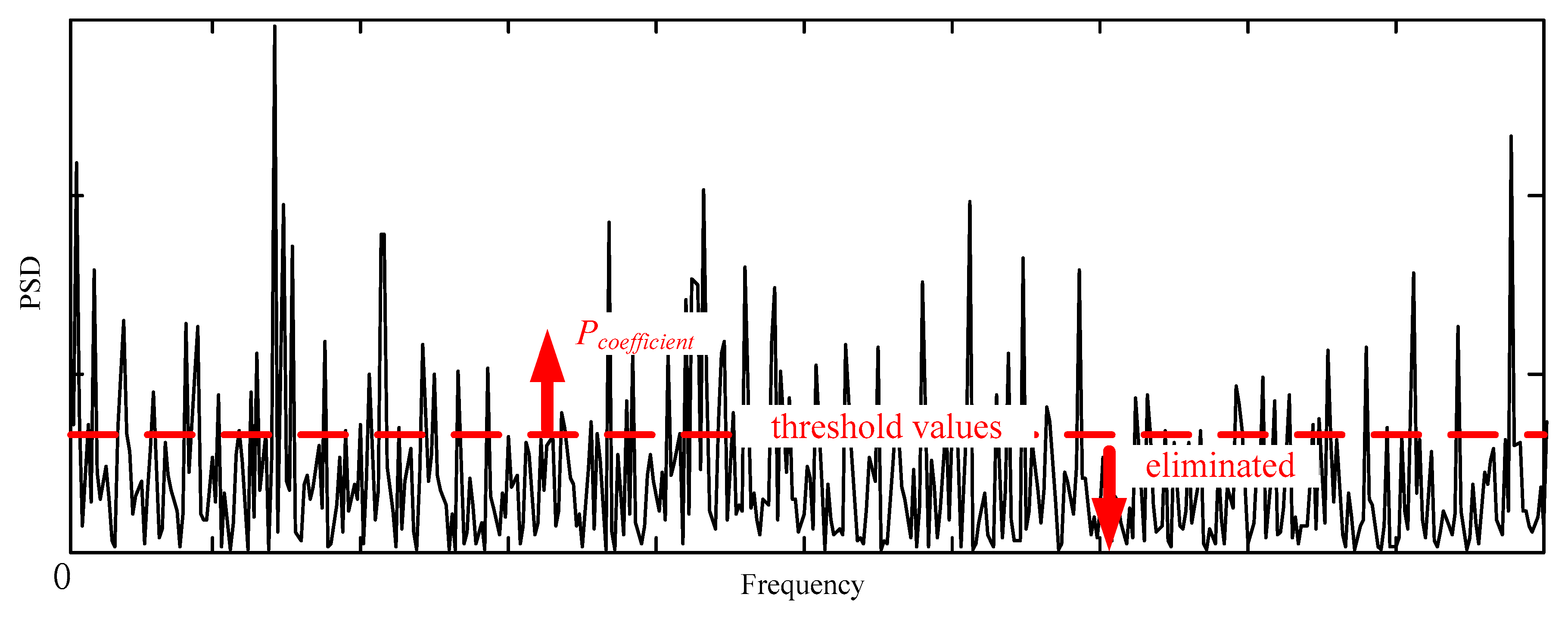
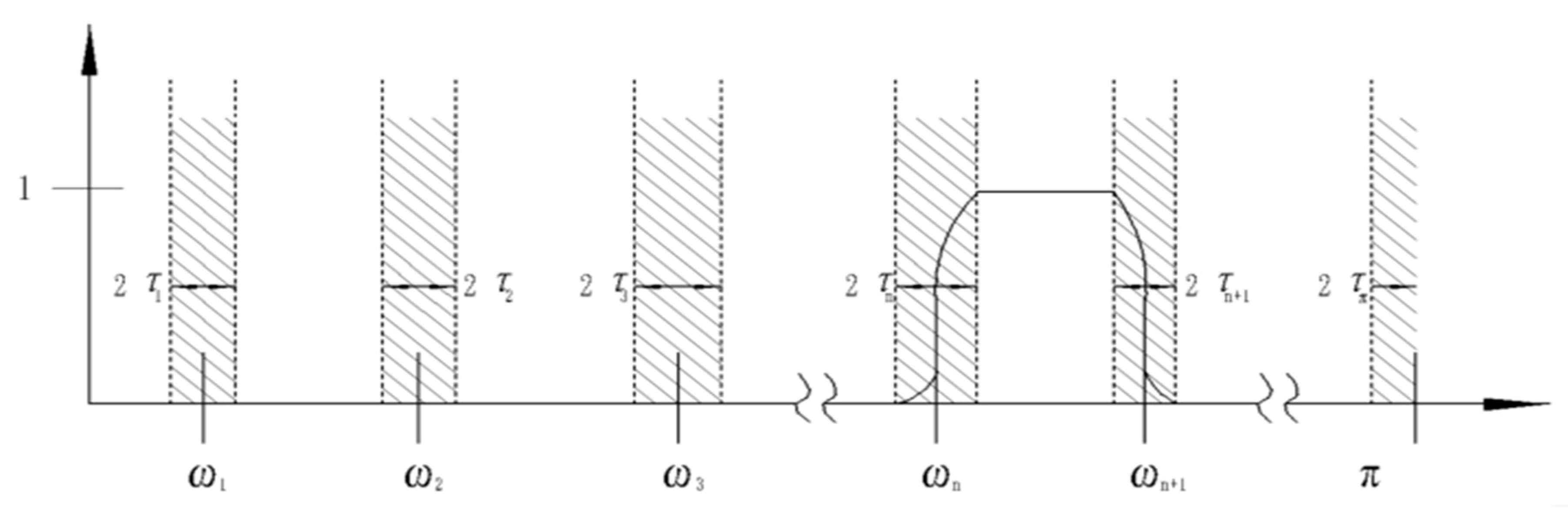
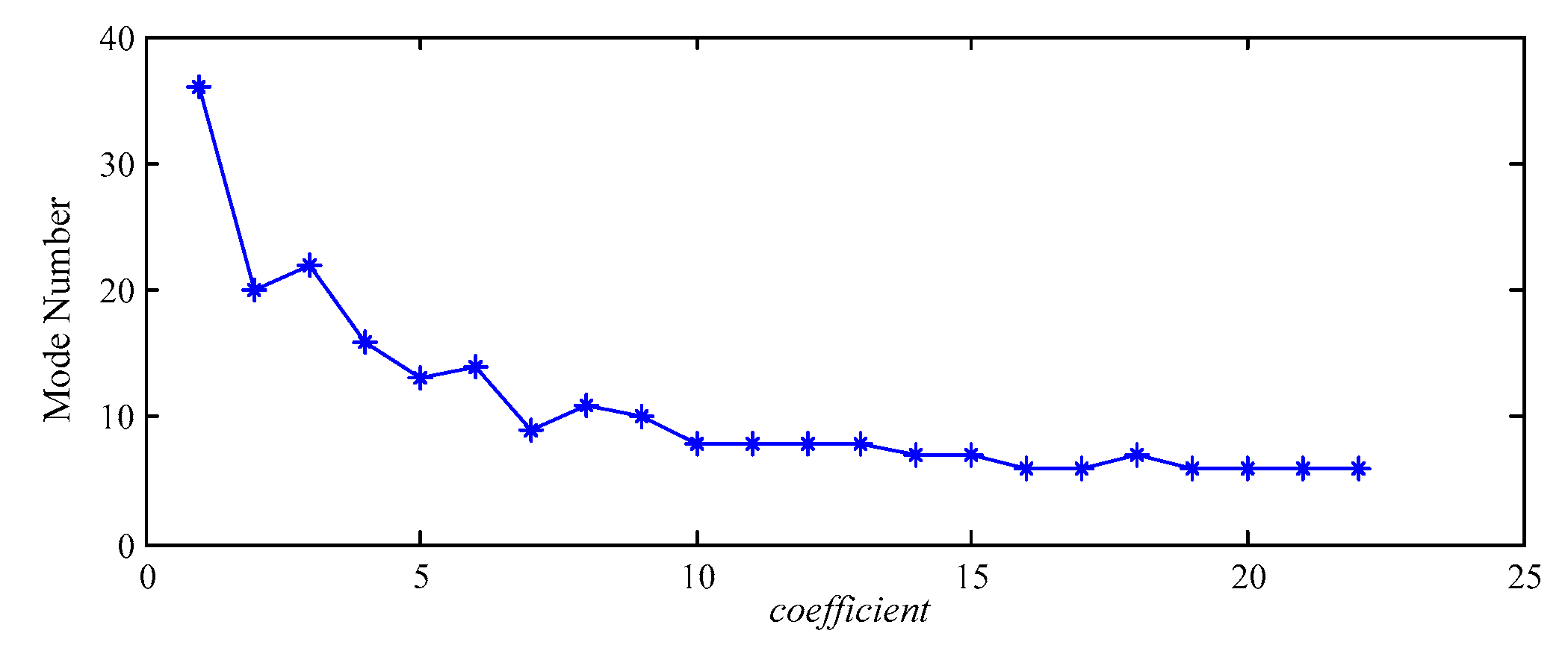
2.2. Improved Empirical Wavelet Transform

The algorithm of IEWT is described as follows:

(1) Calculating power spectrum of signals

Different from the Fourier amplitude spectrum of EWT, IEWT is based on power spectrum.

Let x(t) = (x₁, x₂, …, x_n) be a signal, and X(ω) is its Fourier amplitude spectrum in the frequency domain, and then the power spectrum of the signal is denoted as P, and it is defined as

$$P=\underset{T\to \infty }{\lim }\frac{1}{2T}{{\displaystyle \int }}_{-T}^T{x}^2\left(t\right)dt=\frac{1}{2\pi }{{\displaystyle \int }}_{-\infty }^{\infty }\underset{T\to \infty }{\lim }\frac{1}{2T}{\left|X_T\left(\omega \right)\right|}^{2}d\omega$$

(2)

(2) Applying the threshold processing

The step is also different from EWT, and the threshold processing is introduced into IEWT. The threshold values are defined as

THVA = coefficient × mean(P)

(3)

where coefficient is an integer and equals to 1, 2, …, L.

Figure 1 demonstrates how the threshold processing works.

In Figure 1, the threshold value THVA is applied to eliminate the spectrums whose values are smaller than the values (the eliminated spectrum values are set to 0), and thus a new spectrum distribution P_coefficient can be obtained. Thus, the bad influence of interference components on adaptive segment acquirement is much reduced.

(3) Decomposing the Signals

Periodicity of a normalized Fourier axis is 2 π, and the discussion is restricted to ω ∈ [0, π] based on P_coefficient. It is supposed that the Fourier support [0, π] is segmented into N contiguous segments, which means that there are N + 1 boundaries. However, 0 and π are always used in definition and it is need to be found N − 1 extra boundaries. To find the boundaries, local maxima value of power spectrum are selected, and the values are sorted in decreasing order (0 and π are excluded). It is assumed that the algorithm found M maxima, and two cases can appear:

(1) M ≥ N: enough maxima are selected to define the wanted segment number, and then the first N − 1 maxima are adopted.

(2) M ≤ N: the component mode number of a signal is smaller than expected, and all the selected maxima are kept, and rest N to the appropriate value.

In Figure 2, each segments is defined as Λ_n = [ω_n−1, ω_n], and it can be found that $U_{\mathit{n}=\mathbf{1}}^{\mathit{N}}$ Λ_n = [0, π]. Centered around each ω_n, a transition phase (the gray hatched areas on Figure 2) T_n of width 2τ_n is defined.

Based on construction of Littlewood-Paley and Meyer’s wavelets, some empirical wavelets of EWT are actually band pass filters on each Λ_n. Then ∀n > 0, it can be defined that the empirical scaling function and the empirical wavelets by expressions of Equations (4) and (5) respectively.

$${\widehat{\varnothing }}_n\left(\omega \right)\{\begin{array}{cc}1\hfill & \hfill \mathrm{if} \left|\omega \right|\le {\omega }_n-{\tau }_n\\ \cos \left[\frac{\pi }{2}\beta \left(\frac{1}{2{\tau }_n}\left(\left|\omega \right|-{\omega }_n+{\tau }_n\right)\right)\right]\hfill & \hfill \mathrm{if} {\omega }_n-{\tau }_n\le \left|\omega \right|\le {\omega }_n+{\tau }_n\\ 0\hfill & \hfill \mathrm{otherwise}\end{array}$$

(4)

and

$${\widehat{\varnothing }}_n\left(\omega \right)\{\begin{array}{cc}1\hfill & \hfill \mathrm{if} {\omega }_n+{\tau }_n\le \left|\omega \right|\le {\omega }_{n+1}-{\tau }_{n+1}\\ \cos \left[\frac{\pi }{2}\beta \left(\frac{1}{2{\tau }_{n+1}}\left(\left|\omega \right|-{\omega }_{n+1}+{\tau }_{n+1}\right)\right)\right]\hfill & \hfill \mathrm{if} {\omega }_{n+1}-{\tau }_{n+1}\le \left|\omega \right|\le {\omega }_{n+1}+{\tau }_{n+1}\\ \sin \left[\frac{\pi }{2}\beta \left(\frac{1}{2{\tau }_n}\left(\left|\omega \right|-{\omega }_n+{\tau }_n\right)\right)\right]\hfill & \hfill \mathrm{if} {\omega }_n-{\tau }_n\le \left|\omega \right|\le {\omega }_n+{\tau }_n\\ 0\hfill & \hfill \mathrm{otherwise}\end{array}$$

(5)

where γ<min_n [ω_n+1 − ω_n/ω_n+1 + ω_n], β(x) = 35x⁴ − 8x⁵ + 70x⁶ − 20x⁷.

The definition of IEWT is the same as EWT, and IEWT is defined in the same way as for the classic wavelet transform. Detail coefficient $W_f^{\epsilon }\left(n,t\right)$ is given by the inner products with the empirical wavelets in Equation (6). Approximation coefficient $W_f^{\epsilon }\left(0,t\right)$ is given by the inner products with the scaling function in Equation (7).

$$W_f^{\epsilon }(n,t)=\langle f,{\Psi }_n\rangle ={(f(\omega )\overline{{\widehat{\Psi }}_n(\omega )})}^{˅}$$

(6)

$$W_f^{\epsilon }(0,t)=\langle f,{\varnothing }_1\rangle ={(f(\omega )\overline{{\widehat{\varnothing }}_{1n}(\omega )})}^{˅}$$

(7)

The signal is reconstructed, and it is defined in Equation (8).

$$f(t)=W_f^{\epsilon }(0,t){\varnothing }_1(\omega )+{\displaystyle \sum }_{n=1}^N{W}_f^{ϵ}(n,t){\Psi }_n(t)={({\widehat{W}}_f^{\epsilon }(0,\omega ){\widehat{\varnothing }}_1(\omega )+{\displaystyle \sum }_{n=1}^N{\widehat{W}}_f^{ϵ}(n,\omega ){\widehat{\Psi }}_n(\omega ))}^{˅}$$

(8)

Thus the empirical modes are given in Equations (9) and (10)

$$F_0\left(t\right)=W_f^{\epsilon }\left(0,t\right){\varnothing }_1\left(t\right)$$

(9)

$$F_k\left(t\right)=W_f^{\epsilon }\left(k,t\right){\Psi }_k\left(t\right)$$

(10)

(4) Selecting the best decomposition result based on FER

The step is very important and also different from EWT, and the purpose of the step is to find the best decomposition.

Because coefficient = 1, 2, …, L, there are P₁, P₂, …, P_L, and thus L decomposition results can be got. Each result is comprised of some component modes, and the mode corresponding to the biggest FER value FER_{coefficient, max} is compared with that corresponding to the second biggest FER value FER_{coefficient, max}, and the comparison result is denoted in Equation (11).

A_coefficient = (FER_{coefficient, max} − FER_{coefficient, secondmax})/FER_{coefficient, secondmax}

(11)

Maximum value of A_coefficient is denoted as A_max, and thus A_max corresponds to the best decomposition result, and the corresponding threshold value is the best decomposition value. Therefore, the mode to FER_{coefficient, max} contains the richest fault feature information.

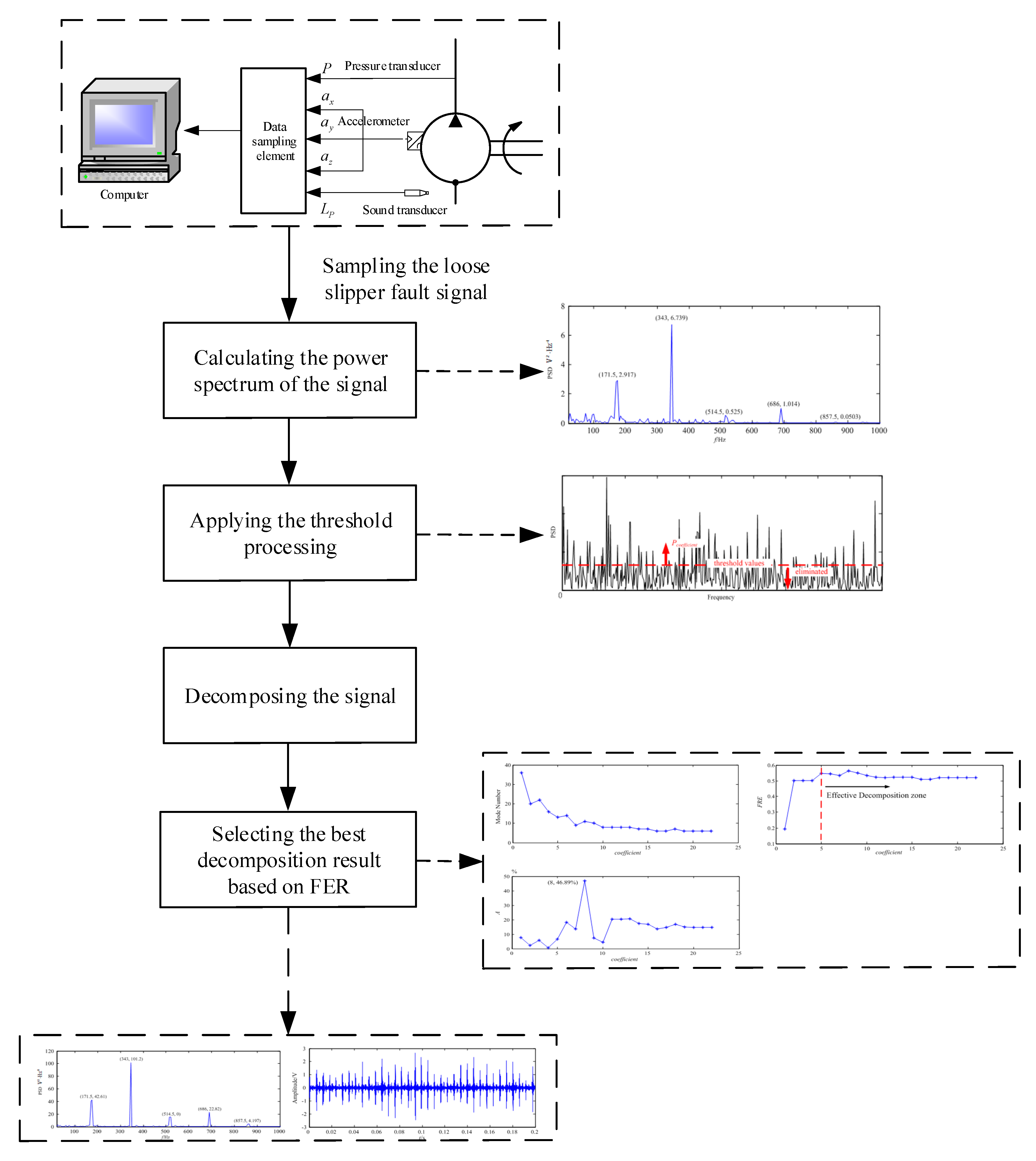
2.3. The Flowchart of IEWT

Firstly, the power spectrum of the loose slipper fault signal is calculated. Secondly, the threshold processing is applied to eliminate the power spectrum of the interference components, and segments can be acquired. Thirdly, the signal can be decomposed by IEWT based on the segments. Lastly, the best decomposition result can be selected by FER.

The flowchart of IEWT is shown in Figure 3.

3. Results and Discussion

3.1. Simualtion Study

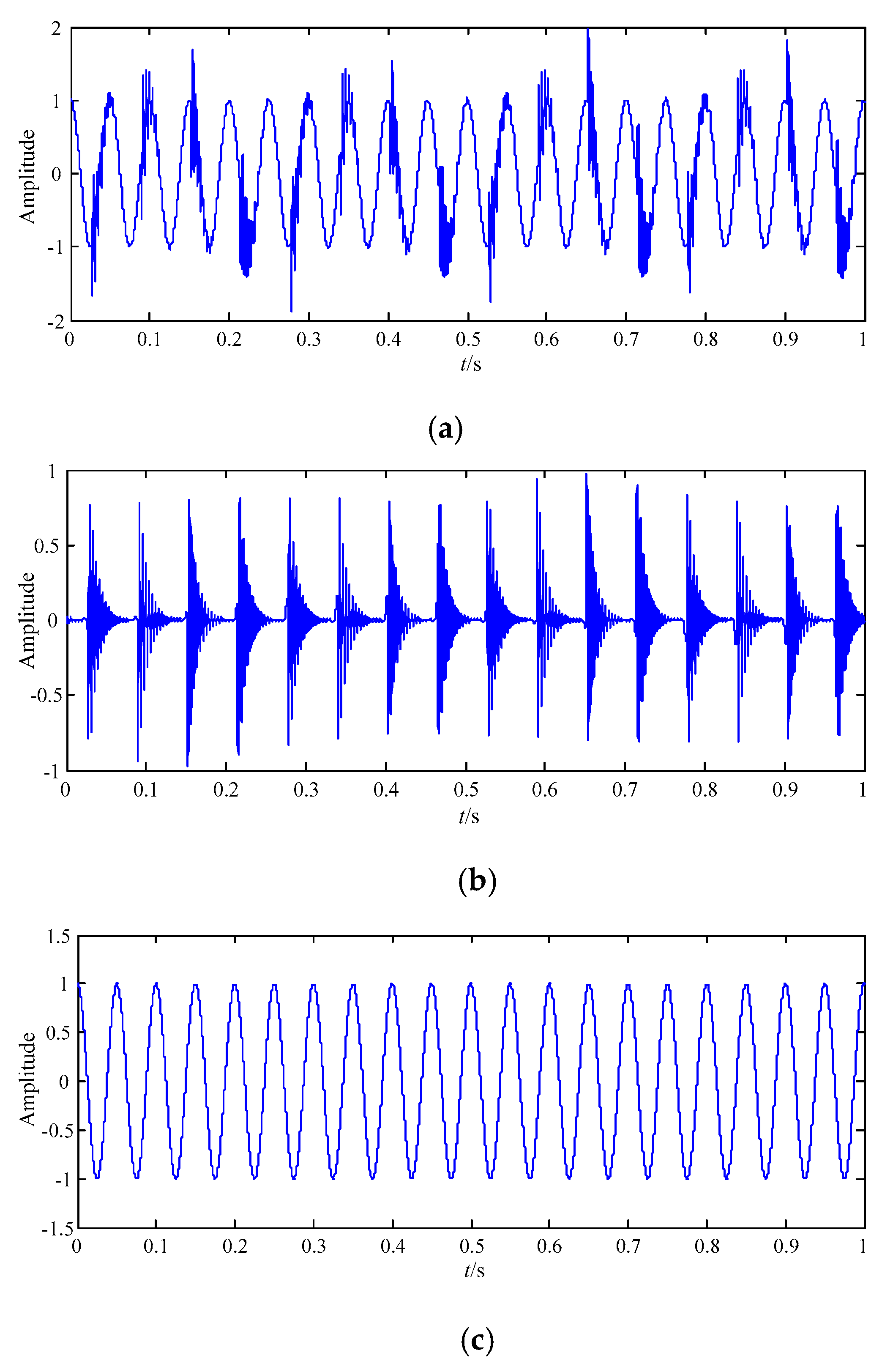
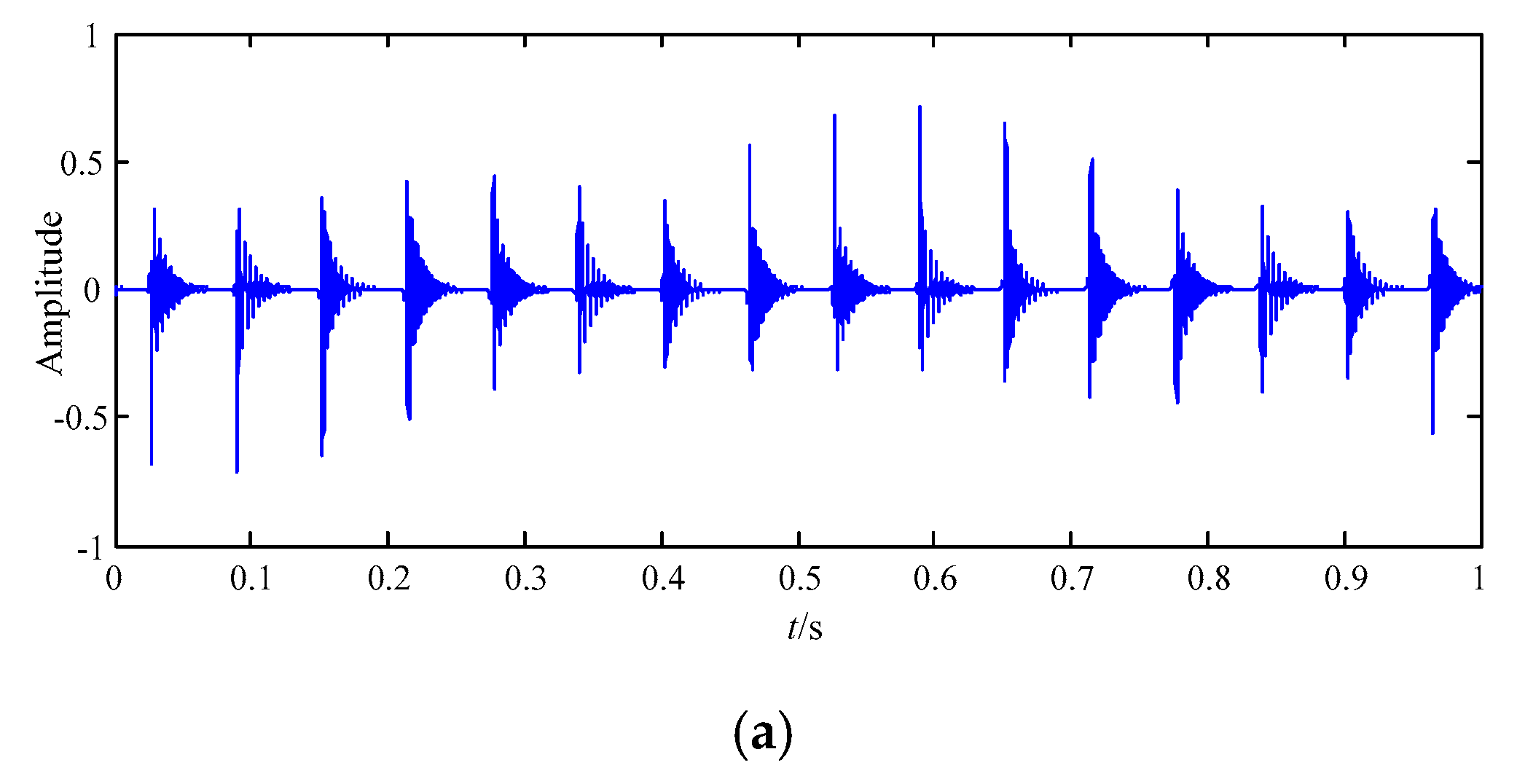
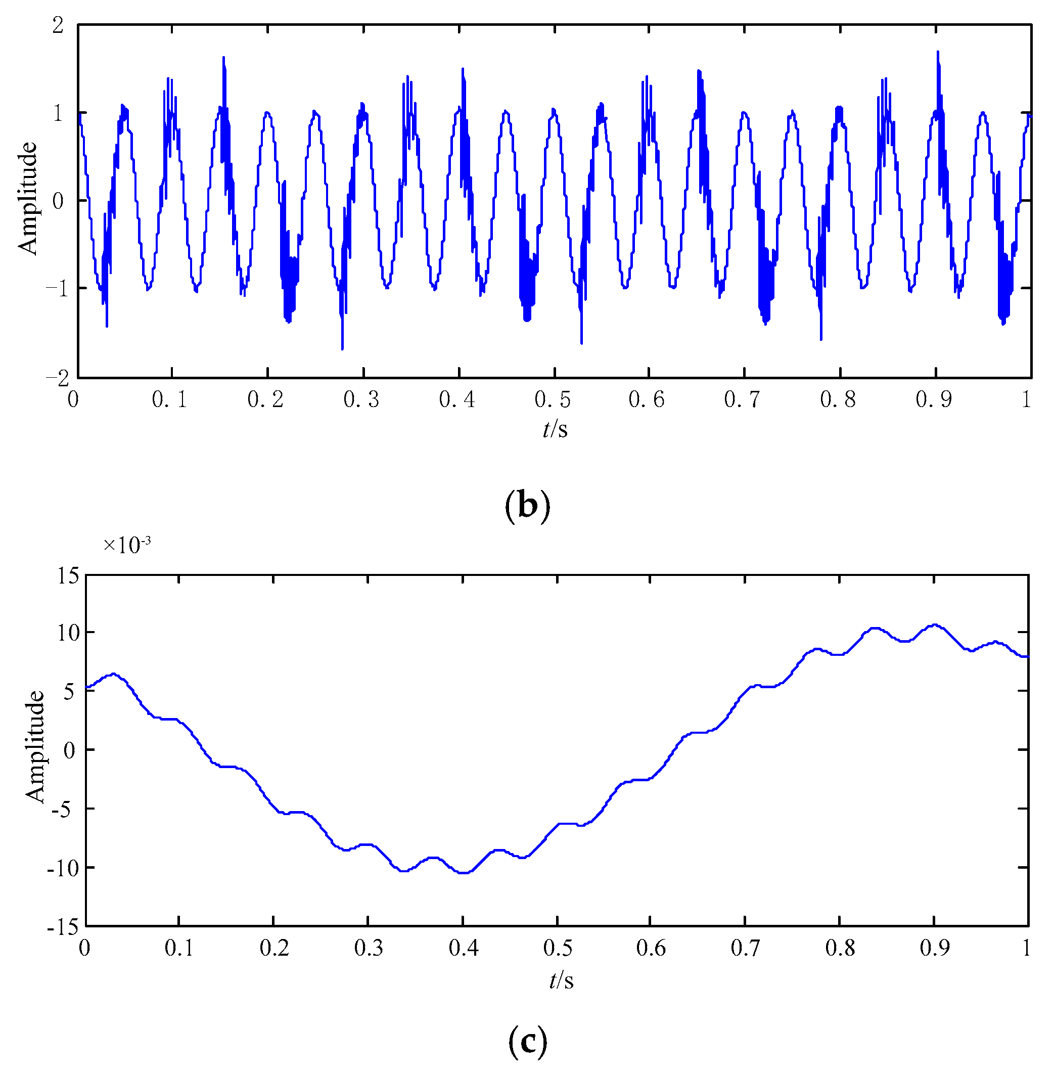
3.1.1. The Simulated Signal

In order to verify the superiority and effectiveness of IEWT, a simulated signal is defined as

x(t) = x₁(t) + x₂(t)

(12)

The signal consists of two component modes of x₁(t) and x₂(t). x₁(t) is used to simulate an impact signal caused by a fault, and it is an impact signal with periodic exponential attenuation, and its periodicity is 16 Hz, and attenuation function is e^−100tsin(510πt) in one periodicity. x₂(t) is a cosine signal, and its periodicity is 20 Hz, and x₂(t) is used to simulate an interference signal of low frequency harmonic. The sampling frequency is 10,240 Hz and sampling time is 1 s.

The signals x(t), x₁(t) and x₂(t) are displayed in Figure 4.

3.1.2. The Simulated Result Analysis Based on EWT

For demonstrating the superiority and effectiveness of IEWT, the simulated signal is also decomposed by EWT. After the decomposition analysis, three modes can be obtained, which means that there are three contiguous segments and four boundaries. Thus, there is over-decomposition, and the decomposition result is shown in Figure 5 and Figure 6.

Figure 5a shows the wave of F₃ in the time domain. Compared with the wave of x₁(t) in Figure 4b, it is shown that the wave of F₃ is distorted. Thus, the periodic impact feature information of F₃ is much different from that of x₁(t).

Figure 5b displays the wave of F₂ in the time domain, and it is seriously interfered with. Compared with the wave of x(t) in Figure 4a, the feature information of F₂ is unexpectedly high similar with that of original signal x(t), but it is known that F₂ is just a mode obtained by EWT, and thus the decomposition is wrong.

Figure 5c depicts the wave of F₁ in the time domain, and its amplitudes are very small. By comparing it with the waves of the three signals of x(t), no signal is the same as the F₁, and its wave is also seriously distorted.

Thus, it is shown that only F₃ is a little similar with the impact signal x₁(t) among the three modes.

Figure 6 shows the spectrum of F₃ in the frequency domain. The fault feature information at fault feature frequency 16 Hz and its harmonics 32 Hz, 48 Hz, 64 Hz, 80 Hz and 96 Hz are all obvious.

It can be concluded from the above analysis that although the F₃ is a little similar with the impact signal x₁(t) in the time domain, there are only two signals in the simulated signal x(t), and there are three modes of F₁, F₂, and F₃ in the decomposition result, and thus x(t) is over-decomposed by EWT.

3.1.3. The Simulated Result Analysis Based on IEWT

The power spectrum of the simulated signal is denoted as P_coefficient, and threshold value THVA is set as coefficient × mean(P_coefficient), where coefficient is an integer and mean (P_coefficient) is mean spectrum value of P_coefficient.

The simulated signal is decomposed by IEWT in [1 122] of the coefficient range, and mode numbers of 122 decomposition results based on different coefficients are displayed in Figure 7.

It can be seen from Figure 7 that the signal can be effectively and correctly decomposed into only two modes of F₁ and F₂ in each decomposition result, which means that there are two contiguous segments and three boundaries. Thus, there is no over-decomposition and mode mixing, and it is no need to compute comparison between the FER_{coefficient, max} and FER_{coefficient, secondmax} in Step 4.

In order to get the best decomposition result, FER of each mode is computed based on each of the 122 results. According to the above FER, it can be seen that the FER value of F₂ (the highest-order mode) is the biggest in each result, which means that each F₂ contains the richest fault feature information. FER value of each F₂ in all decomposition results is revealed in Figure 8.

It can be known from Figure 8 that FER values in [1 122] of the coefficient range are all above 0.9, and their trend tends to be stable in the range, and all of the biggest values are 0.936 in [61 122]. Thus, the best decomposition result is in [61 122], and all of the results are the same in the range, so only the best result based on coefficient = 61 is shown in Figure 9 and Figure 10.

The wave of F₂ is shown in Figure 9a, and it displays the periodic impact feature information in the time domain. It is compared with the wave of x₁(t) in Figure 4b, and there is nearly no difference between them. Therefore, it is concluded that periodic impact feature information of F₂ is high similar with that of x₁(t) in the time domain.

Figure 9b displays the feature information of cosine curve in F₁, and it is contaminated by little interferences. By comparing the wave of F₁ with that of x₂(t) in Figure 4c, it can be seen that feature information of F₁ is high similar with that of cosine signal x₂(t) in the time domain.

Figure 10 shows the spectrum of F₂ in the frequency domain. The amount of the fault feature information at fault feature frequency 16 Hz and its harmonics 32 Hz, 48 Hz, 64 Hz, 80 Hz and 96 Hz is very large, thus the fault feature information is extracted effectively, and there are nearly no interference components in other frequencies.

It can be known that F₂ got by IEWT and F₃ got by EWT are modes which contain the most of fault feature information, thus the two are compared with each other in the time and frequency domains. The similarity between time waves of F₂ and that of x₁(t) is higher than that between time waves of F₃ and that of x₁(t) in the time domain; the fault feature information amount of F₂ is larger than that of F₃ in the frequency domain.

From the above analysis, it is concluded that the segment can be set according to Fourier power density spectrum in the effective way, and the right mode number can be got, and then one mode which contains the richest feature information can be selected based on FER, and thus the simulated signal can be best decomposed by IEWT. Moreover, there is no over-decomposition and mode mixing, so IEWT performs much better than EWT.

3.2. Application to Fault Signals of Hydraulic Pump

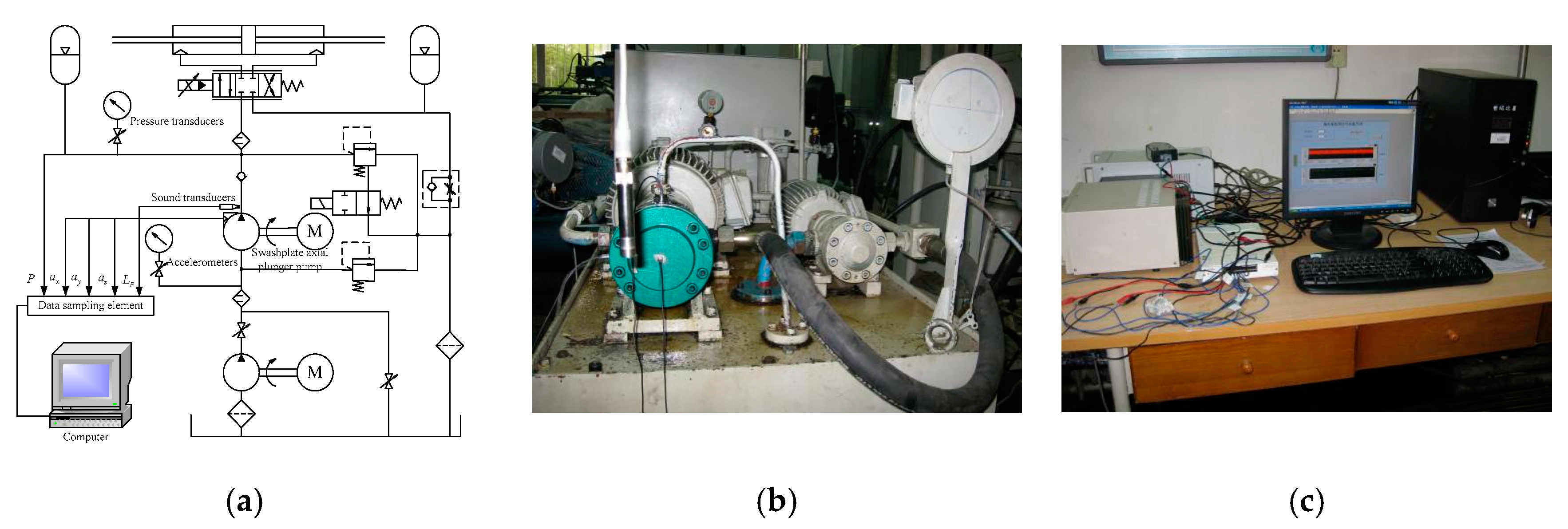
3.2.1. Experimental Scheme

An experiment was performed to swash plate axial plunger pump whose type was 10MCY14-1B. Its rotational speed was set as 1470 r/min, and outlet pressure of the pump was set as 15 MPa. The signals of loose slipper fault are sampled by accelerometer a_z at frequency of 50 kHz. The two kinds of fault feature frequency are 171.5 Hz [35]. The experimental system is displayed in Figure 11.

The length of the loose slipper fault signal is 0.2 s, and the signal is shown in Figure 12.

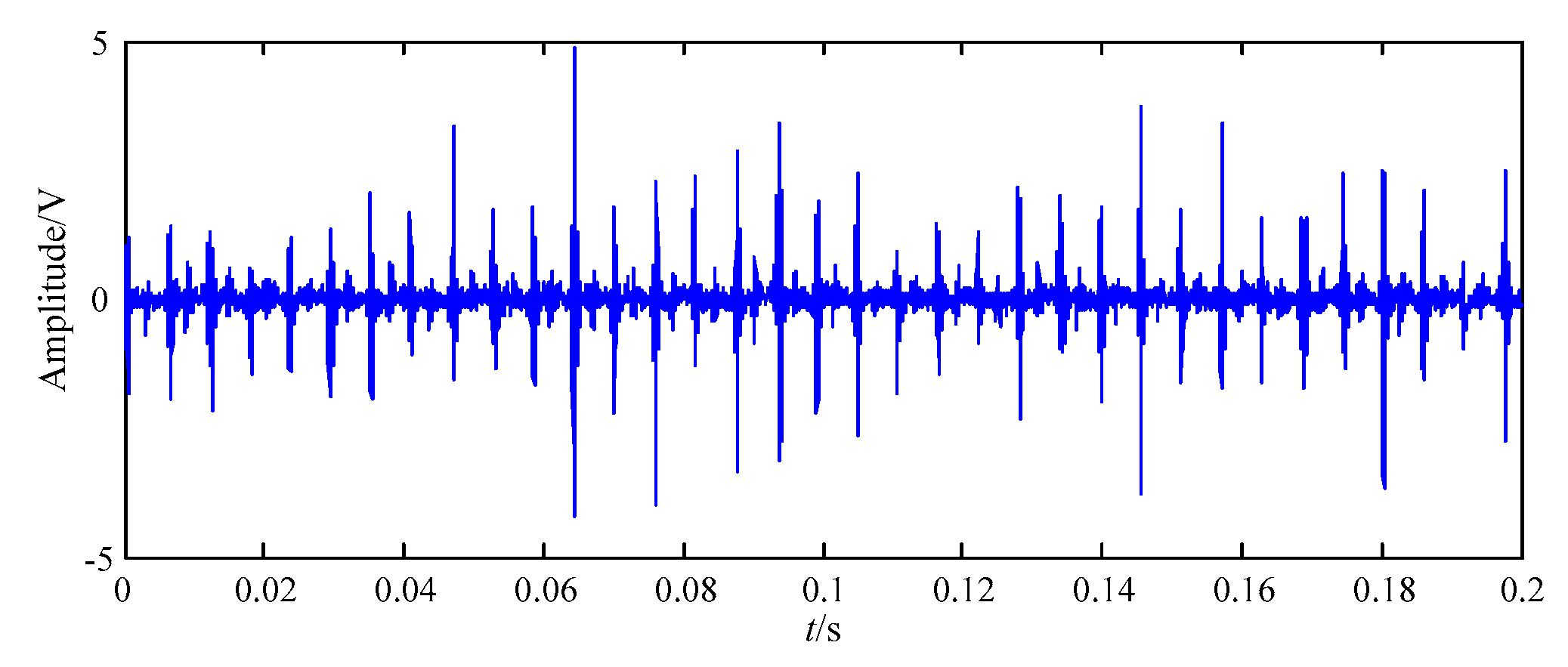
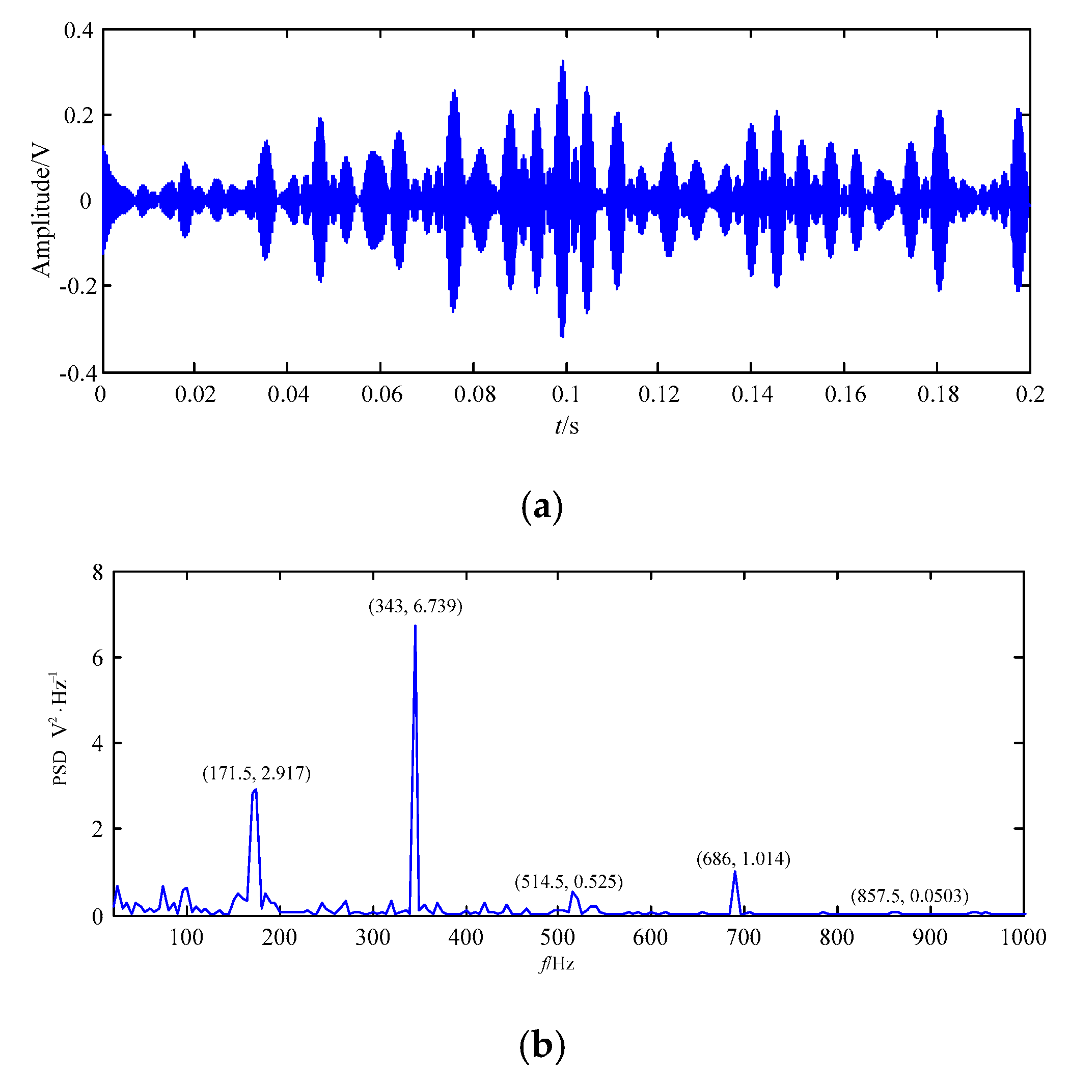
3.2.2. The Application to the Loose Slipper Fault Signal Based on EWT

In order to validate the superiority and effectiveness of IEWT, the loose slipper fault signal is firstly decomposed by EWT, and 58 modes can be obtained, so there is serious over-decomposition. The F₁₃ corresponds to maximum FER value, thus the mode contains the largest amount of fault feature information, and F₁₃ is displayed in Figure 13.

In Figure 13a, the wave of F₁₃ is displayed, and the periodic impact feature information is a little obvious, but the periodicity and amplitude information is very irregular. The fault feature information of F₁₃ in Figure 13a is low, similar with that of the original loose slipper fault signal in Figure 12.

The spectrum of F₁₃ is displayed in Figure 13b. In the frequency domain, the fault feature information at fault feature frequency 171.5 Hz and some of its harmonics is obvious, and there are some noises in the other frequencies.

3.2.3. The Application to the Loose Slipper Fault Signal Based on IEWT

IEWT is also applied to decompose the signal in [1 22] of the coefficient range, where the power spectrum of the loose slipper fault signal is denoted as P_coefficient, the threshold value THVA is set as coefficient × mean (P_coefficient), coefficient is an integer, and mean (P_coefficient) is mean value of P_coefficient.

The mode number of each decomposition result is obtained based on the different coefficients, as displayed in Figure 14.

From Figure 14, the mode number decreases with the increase of coefficient in all results. There are 36 modes in the case of coefficient = 1, which means that there are 36 contiguous segments and 37 boundaries. All of the results have six modes in the case of coefficient = 19–21. Thus, 36 modes mean that there is over-decomposition, and six modes indicate that there is mode mixing.

For the sake of obtaining the best decomposition result, FER of each mode is computed in each of all 22 results and the FER value of the highest-order mode is the biggest in each result. The FER value of each highest-order mode in all decompositions is displayed in Figure 15.

In the case of coefficient ≥ 5, FER values change little and maintain at the maximum in Figure 15. Thus, the reasonable decomposition result is in [5 22].

In order to get the best decomposition result, it is necessary to figure out whether there ia over-decomposition and mode mixing in each result. FER_{coefficient, max} of the highest-order mode is compared with FER_{coefficient, secondmax} of a certain mode in each result. If the above two FERs are very close, there is a real possibility that there is over-decomposition and mode mixing in this result. Comparison result of FER_{coefficient, max} and FER_{coefficient, secondmax} in each result is demonstrated in Figure 16.

In the case of coefficient = 8, it can be found that A_max = 46.89% in Figure 16, and it can be also seen that F₁₁ is the highest-order mode in Figure 14, which means that there are 11 contiguous segments and 12 boundaries in the result. FER_{8, max} corresponding to F₁₁ is 0.5644, and FER_{4, max} corresponding to F₄ is 0.3842. FER_{8, max} is 46.90% bigger than FER_{4, max}, and thus there is a real possibility that there is no over-decomposition and mode mixing in the case of coefficient = 8. The best decomposition result of IEWT can be obtained, as displayed in Figure 17 and Figure 18.

It can be seen from Figure 17 that periodic impact feature information of the highest-order mode F₁₁ is more obvious than that of F₁–F₁₀, and that of F₁₁ is high similar with that of the original loose slipper fault signal in Figure 12. The spectrum of F₁₁ is shown in Figure 18a, the amplitudes at fault feature frequency 171.5 Hz and its harmonics are all obvious; in Figure 18a–k, the amplitudes at the above frequencies are not all extracted in the spectrum of F₁–F₁₀, and there are many interference components in other frequencies. Thus, F₁₁ contains the largest amount of fault feature information.

Compared with F₁₃ got by EWT in Figure 13a, the periodic impact feature information of F₁₁ got by IEWT is very obvious and regular in Figure 17a, and the amplitudes of F₁₁ are also much higher than those of F₁₃. By comparing with F₁₃ got by EWT in Figure 13b, it can be seen that the amplitudes of F₁₁ got by IEWT at the fault feature frequency and its harmonics are all extracted, and the amount of fault feature information is much larger than that of F₁₃.

It can be concluded from the above analysis that the right segment can be obtained according to Fourier power density spectrum, and then the effective mode number is obtained. Based on the mode number, the best decomposition of the loose slipper fault signal can be got by IEWT in the case of coefficient = 8, and then the mode which contains the richest fault feature information can be selected based on FER. Moreover, it performs better than EWT.

4. Conclusions

When the hydraulic pump works, it is often faced with of high pressure and high speed working conditions. The vibration of the hydraulic pump is usually caused by mechanical and fluid impact, and the vibration is intensified if it is broken, and thus the fault vibration signal is contaminated by a lot of noises. The Fourier amplitude spectrum is sensitive to the noises, and the segment is got based the above spectrum of the contaminated fault signal in EWT, and thus the signal is decomposed in the wrong way.

Aiming to resolve the shortcomings of EWT, an improved method IEWT is proposed, and IEWT replaced the Fourier amplitude spectrum of EWT with power spectrum in acquiring the segment, and thus the bad influence of the interference on the segment acquirement is much reduced. Based on the right segment, the loose slipper fault signal can be decomposed by IEWT in the best way, and the mode that contains the most amount of the fault feature information can be selected based on FER. Therefore, mode-mixing and over-decomposition can be eliminated as much as possible, and IEWT performs much better than EWT.

References

1. Qian, J.Y.; Chen, M.R.; Liu, X.L.; Jin, Z.J. A numerical investigation of the flow of nanofluids through a micro Tesla valve. J. Zhejiang Univ. Sci. A 2019, 20, 50–60. [Google Scholar] [CrossRef]
2. Qian, J.-Y.; Gao, Z.-X.; Liu, B.-Z.; Jin, Z.-J. Parametric Study on Fluid Dynamics of Pilot-Control Angle Globe Valve. J. Fluids Eng. 2018, 140, 111103. [Google Scholar] [CrossRef]
3. Zhu, Y.; Qian, P.; Tang, S.; Jiang, W.; Li, W.; Zhao, J. Amplitude-frequency characteristics analysis for vertical vibration of hydraulic AGC system under nonlinear action. AIP Adv. 2019, 9, 035019. [Google Scholar] [CrossRef] [Green Version]
4. Zhu, Y.; Tang, S.; Quan, L.; Jiang, W.; Zhou, L. Extraction method for signal effective component based on extreme-point symmetric mode decomposition and Kullback–Leibler divergence. J. Braz. Soc. Mech. Sci. Eng. 2019, 41, 100. [Google Scholar] [CrossRef]
5. Wang, C.; Chen, X.; Qiu, N.; Zhu, Y.; Shi, W. Numerical and experimental study on the pressure fluctuation, vibration, and noise of multistage pump with radial diffuser. J. Braz. Soc. Mech. Sci. Eng. 2018, 40, 481. [Google Scholar] [CrossRef]
6. Wang, C.; Hu, B.; Zhu, Y.; Wang, X.; Luo, C.; Cheng, L. Numerical Study on the Gas-Water Two-Phase Flow in the Self-Priming Process of Self-Priming Centrifugal Pump. Processes 2019, 7, 330. [Google Scholar] [CrossRef]
7. Zhang, J.; Xia, S.; Ye, S.; Xu, B.; Song, W.; Zhu, S.; Tang, H.; Xiang, J. Experimental investigation on the noise reduction of an axial piston pump using free-layer damping material treatment. Appl. Acoust. 2018, 139, 1–7. [Google Scholar] [CrossRef]
8. Ye, S.; Zhang, J.; Xu, B.; Zhu, S.; Xiang, J.; Tang, H. Theoretical investigation of the contributions of the excitation forces to the vibration of an axial piston pump. Mech. Syst. Signal Process. 2019, 129, 201–217. [Google Scholar] [CrossRef]
9. Lan, Y.; Hu, J.; Huang, J.; Niu, L.; Zeng, X.; Xiong, X.; Wu, B. Fault diagnosis on slipper abrasion of axial piston pump based on Extreme Learning Machine. Measurement 2018, 124, 378–385. [Google Scholar] [CrossRef]
10. Sun, H.; Yuan, S.; Luo, Y. Cyclic Spectral Analysis of Vibration Signals for Centrifugal Pump Fault Characterization. IEEE Sens. J. 2018, 18, 2925–2933. [Google Scholar] [CrossRef]
11. Zhao, Z.; Jia, M.; Wang, F.; Wang, S. Intermittent chaos and sliding window symbol sequence statistics-based early fault diagnosis for hydraulic pump on hydraulic tube tester. Mech. Syst. Signal Process. 2009, 23, 1573–1585. [Google Scholar] [CrossRef]
12. Du, J.; Wang, S.; Zhang, H. Layered clustering multi-fault diagnosis for hydraulic piston pump. Mech. Syst. Signal Process. 2013, 36, 487–504. [Google Scholar] [CrossRef]
13. Lu, C.; Wang, S.; Makis, V. Fault severity recognition of aviation piston pump based on feature extraction of EEMD paving and optimized support vector regression model. Aerosp. Sci. Technol. 2017, 67, 105–117. [Google Scholar] [CrossRef]
14. Sharma, P.; Newman, K.; Long, C.; Gasiewski, A.; Barnes, F. Use of wavelet transform to detect compensated and decompensated stages in the congestive heart failure patient. Biosensors 2017, 7, 40. [Google Scholar] [CrossRef]
15. Zin, Z.M.; Salleh, S.H.; Daliman, S.; Sulaiman, M.D. Analysis of heart sounds based on continuous wavelet transform. In Proceedings of the IEEE Student Conference on Research and Development, Putrajaya, Malaysia, 25–26 August 2003. [Google Scholar]
16. Tsalaile, T.; Sanei, S. Separation of heart sound signal from lung sound signal by adaptive line enhancement. In Proceedings of the European Signal Processing Conference, Poznan, Poland, 3–7 September 2007. [Google Scholar]
17. El-Asir, B.; Khadra, L.; Al-Abbasi, A.H.; Mohammed, M.M.J. Time-frequency analysis of heart sounds. In Proceedings of the Digital Processing Applications (TENCON ′96), Perth, WA, Australia, 26–29 November 1996. [Google Scholar]
18. Li, Y.; Liang, X.; Xu, M.; Huang, W. Early fault feature extraction of rolling bearing based on ICD and tunable Q-factor wavelet transform. Mech. Syst. Signal Process. 2017, 86, 204–223. [Google Scholar] [CrossRef]
19. Singh, J.; Darpe, A.; Singh, S.; Singh, S. Rolling element bearing fault diagnosis based on Over-Complete rational dilation wavelet transform and auto-correlation of analytic energy operator. Mech. Syst. Signal Process. 2018, 100, 662–693. [Google Scholar] [CrossRef]
20. Kordestani, M.; Samadi, M.F.; Saif, M.; Khorasani, K. A New Fault Diagnosis of Multifunctional Spoiler System Using Integrated Artificial Neural Network and Discrete Wavelet Transform Methods. IEEE Sens. J. 2018, 18, 4990–5001. [Google Scholar] [CrossRef]
21. Zhao, M.; Kang, M.; Tang, B.; Pecht, M. Deep residual networks with dynamically weighted wavelet coefficients for fault diagnosis of planetary gearboxes. IEEE Trans. Ind. Electron. 2018, 65, 4290–4300. [Google Scholar] [CrossRef]
22. Song, L.; Wang, H.; Chen, P. Vibration-Based Intelligent Fault Diagnosis for Roller Bearings in Low-Speed Rotating Machinery. IEEE Trans. Instrum. Meas. 2018, 67, 1887–1899. [Google Scholar] [CrossRef]
23. Huang, N.E. The Empirical Mode Decomposition and the Hilbert Spectrum for Nonlinear and Non-stationary Time Series Analysis. Proc. Math. Phys. Eng. Sci. 1998, 454, 903–995. [Google Scholar] [CrossRef]
24. Yang, W.; Court, R.; Tavner, P.J.; Crabtree, C.J. Bivariate empirical mode decomposition and its contribution to wind turbine condition monitoring. J. Sound Vib. 2011, 330, 3766–3782. [Google Scholar] [CrossRef]
25. Liu, H.; Zhang, J.; Cheng, Y.; Lu, C. Fault diagnosis of gearbox using empirical mode decomposition and multi-fractal detrended cross-correlation analysis. J. Sound Vib. 2016, 385, 350–371. [Google Scholar] [CrossRef]
26. Osman, S.; Wang, W. An enhanced Hilbert–Huang transform technique for bearing condition monitoring. Meas. Sci. Technol. 2013, 24, 085004. [Google Scholar] [CrossRef]
27. Li, Y.; Xu, M.; Liang, X.; Huang, W. Application of Bandwidth EMD and Adaptive Multiscale Morphology Analysis for Incipient Fault Diagnosis of Rolling Bearings. IEEE Trans. Ind. Electron. 2017, 64, 6506–6517. [Google Scholar] [CrossRef]
28. Zhang, J.; Huang, D.; Yang, J.; Liu, H.; Liu, X. Realizing the empirical mode decomposition by the adaptive stochastic resonance in a new periodical model and its application in bearing fault diagnosis. J. Mech. Sci. Technol. 2017, 31, 4599–4610. [Google Scholar] [CrossRef]
29. Pan, H.; Yang, Y.; Li, X.; Zheng, J.; Cheng, J. Symplectic geometry mode decomposition and its application to rotating machinery compound fault diagnosis. Mech. Syst. Signal Process. 2019, 114, 189–211. [Google Scholar] [CrossRef]
30. Gilles, J. Empirical Wavelet Transform. IEEE Trans. Signal Process. 2013, 61, 3999–4010. [Google Scholar] [CrossRef]
31. Wang, D.; Zhao, Y.; Yi, C.; Tsui, K.-L.; Lin, J. Sparsity guided empirical wavelet transform for fault diagnosis of rolling element bearings. Mech. Syst. Signal Process. 2018, 101, 292–308. [Google Scholar] [CrossRef]
32. Jiang, X.; Wu, L.; Ge, M. A Novel Faults Diagnosis Method for Rolling Element Bearings Based on EWT and Ambiguity Correlation Classifiers. Entropy 2017, 19, 231. [Google Scholar] [CrossRef]
33. Cao, H.; Fan, F.; Zhou, K.; He, Z. Wheel-bearing fault diagnosis of trains using empirical wavelet transform. Measurement 2016, 82, 439–449. [Google Scholar] [CrossRef]
34. Shen, L.; Zhou, X.; Zhang, W. Application of morphological demodulation in gear fault feature extraction. J. Zhejiang Univ. Eng. Sci. 2010, 44, 1514–1519. [Google Scholar]
35. Jiang, W.; Zheng, Z.; Zhu, Y.; Li, Y. Demodulation for hydraulic pump fault signals based on local mean decomposition and improved adaptive multiscale morphology analysis. Mech. Syst. Signal Process. 2015, 58, 179–205. [Google Scholar] [CrossRef]
Figure 1. Demonstration of threshold processing.
Processes 07 00824 g001
Figure 2. Segments of the Fourier axis.
Processes 07 00824 g002
Figure 3. The flowchart of improved empirical wavelet transform (IEWT).
Processes 07 00824 g003
Figure 4. The time domain wave of the simulated signal. (a) x(t); (b) x1(t); (c) x2(t).
Processes 07 00824 g004
Figure 5. The results of the simulated signal based on empirical wavelet transform (EWT). (a) F3; (b) F2; (c) F1.
Processes 07 00824 g005aProcesses 07 00824 g005b
Figure 6. Power spectrum density of F3.
Processes 07 00824 g006
Figure 7. The distribution diagram of mode numbers based on the simulated signal.
Processes 07 00824 g007
Figure 8. The feature energy ratio (FER) value distribution diagram of all F2 based on the simulated signal.
Processes 07 00824 g008
Figure 9. The best decomposition results of the simulated signal based on IEWT in the time domain. (a) F2; (b) F1.
Processes 07 00824 g009aProcesses 07 00824 g009b
Figure 10. Power spectrum density of F2.
Processes 07 00824 g010
Figure 11. The experiment system of the swash plate axial plunger pump. (a) Schematic diagram; (b) swash plate axial plunger pump; (c) data acquisition equipment.
Processes 07 00824 g011
Figure 12. The loose slipper fault signal.
Processes 07 00824 g012
Figure 13. F13 got based on EWT. (a) Time domain wave; (b) power spectrum density.
Processes 07 00824 g013
Figure 14. The distribution diagram of mode numbers based on loose slipper fault signal.
Processes 07 00824 g014
Figure 15. The FER value distribution diagram of all highest-order modes based on the loose slipper fault signal.
Processes 07 00824 g015
Figure 16. The comparison distribution diagram of FER based on the loose slipper fault signal.
Processes 07 00824 g016
Figure 17. The best decomposition result of loose slipper fault signal based on IEWT in the time domain. (a) F11; (b) F10; (c) F9; (d) F8; (e) F7; (f) F6; (g) F5; (h) F4; (i) F3; (j) F2; (k) F1.
Processes 07 00824 g017aProcesses 07 00824 g017bProcesses 07 00824 g017c
Figure 18. The best decomposition results of the loose slipper fault signal based on IEWT in the frequency domain. (a) F11; (b) F10; (c) F9; (d) F8; (e) F7; (f) F6; (g) F5; (h) F4; (i) F3; (j) F2; (k) F1.
Processes 07 00824 g018aProcesses 07 00824 g018bProcesses 07 00824 g018c