A Time-Sequence Simulation Method for Power Unit’s Monthly Energy-Trade Scheduling with Multiple Energy Sources

Abstract

The uncertainty of new energy output from wind power is rarely considered in the monthly energy-trade scheduling. This causes many problems since the new energy penetration level increases. The fairness of the scheduled energy for the power suppliers is difficult to guarantee. Because the actual power system operation is far away from scheduling when the monthly energy-trade schedule is carried out, unnecessary wind curtailment might occur, and even the feasibility of monthly energy-trade schedule might not be guaranteed. This affects the security and reliability of the power system operation. In this paper, a new time-sequence simulation method for the monthly energy-trade scheduling is proposed, which considers the new energy power forecasting characteristic and the computational load problem of hourly energy-trade simulation in the remaining months. The proposed method is based on a segment modelling strategy. The power generation in the scheduling month is optimized hourly, and the energy generation is optimized in the subsequent months on a monthly basis. For the scheduling month, accurate cost function is applied in the objective function, and detailed short-term operation constraints and the new energy forecasting results are considered, which can guarantee the feasibility of the new monthly energy-trade scheduling and lay a solid foundation for daily dispatching. For the subsequent months, since the load forecast accuracy is lower and no wind power forecasting results could be used, the rough cost function is applied, and only monthly constraints are considered. To ensure a balance in the execution progress of each power generating entity, the simulation time-scale is set as the remainder of the months in the study year. The new approach ensures the fairness of power execution progress and improves the new energy consumption level. A case study was used to verify the feasibility and effectiveness of the proposed method, which provides a theoretical reference for the monthly electrical energy-trade scheduling.

1. Introduction

Among the generation scheduling processes in China, the annual contract energy planning is carried out according to the contract energy of the generating companies and the national scheduled energy. Then, the monthly energy-trade scheduling and daily generation dispatching are performed by shortening the time scale [1]. Monthly energy-trade scheduling is the intermediate link between the annual contract planning and daily dispatching. If the monthly energy-trade scheduling is improper, the annual contract energy may become difficult to complete. Therefore, the daily dispatching feasibility, operation economy, and security is impacted.

At present, most of the provincial power trading centers in China apply the average decomposition method for monthly energy-trade scheduling. In past decades, the average decomposition method was sufficient to solve the principal contradiction of the power balance. However, this method may be very simple and easy to be implement, but its predominant factors such as the operation condition are not comprehensive enough [2]. Moreover, since the end of the 20th century, with the increasing energy gap and deteriorating ecology, the other drawbacks of the average decomposition method, i.e., lack of energy conservation and emission reduction techniques, have become increasingly prominent. Realizing these drawbacks, some studies [3,4] optimized the formulation of monthly energy-trade scheduling with respect to energy-saving power generation. For instance, a study [3] proposed the combination scheme and calculation method for the non-heating thermal power units of monthly energy-trade scheduling with regard to coal consumption and pollutant emission. Another study [4] expanded the optimization space of energy savings and emission reduction benefits from the time dimension, by optimizing the monthly unit commitment and the current electrical energy distribution. Some improved methods of the conventional units based on the average decomposition method can be found in Reference [5,6,7]. In the monthly trade scheduling method proposed in Reference [5], the deviation of the load ratio was adjusted moderately, according to the comprehensive cost ranking results of the generation unit cost. A comprehensive consumption cost optimization method is proposed in Reference [6], which considers the impact of the monthly electric energy nonlinear fluctuation on the relational consumption cost. On the basis of the unit electric energy integrative cost diversity of different generation units, a new monthly energy-trade scheduling method is proposed in Reference [7], in which the unit electric energy integrative cost of the generation unit was weight-modified. The balance between the economic benefits, energy conservation, and emission reduction can be achieved using the method in Reference [7]. These research works considered the interests of generation units and power grid companies, as well as the social environment. As a result, the benefits of energy saving and emission reduction could be obtained, to some extent, in monthly energy-trade scheduling. However, these research works did not consider the environmental benefits of integrating renewable energy resources into the monthly power trade scheduling process.

In the existing research, the renewable energy units and the conventional units were mostly considered respectively and serially in the monthly energy-trade scheduling. In other words, the remaining load power was reserved for the traditional units in the monthly energy-trade scheduling once the renewable energy power generation is deducted, according to the total load power. This method is feasible when the penetration level of renewable energy is low. However, with the increasing penetration of renewable energy, generation scheduling of thermal power units is influenced by the high volatility, randomness, and intermittence of the renewable energy. A study [8] proposed a market clearing model for energy and reserve products, in coordinated power and gas networks with the integration of compressed air energy storage and wind energy sources (WES), based on two-stage stochastic network-constrained unit commitment. In Reference [9], a sustainable day-ahead scheduling of the grid-connected home-type micro-grids with the integration of distributed energy resources and responsive load demand was co-investigated, and an efficient energy management system optimization algorithm was studied. A novel control algorithm for joint demand response management and thermal comfort optimization in micro-grids equipped with renewable energy sources and energy storage units was presented in Reference [10]. In Reference [11], a simulation-based optimization approach for the design of an EMS in grid-connected photovoltaic-equipped micro-grids with a heterogeneous occupancy schedule was presented. The research studies above could effectively cope with the energy-optimizing problems with large-scale integration of renewable energy into the grid. However, these research studies were all for the micro-grids, which were very different from the regional power grid studied in this paper, and the optimizing time scale is also different from this paper. For the monthly energy-trade scheduling problem with the large-scale integration of renewable energy studied in this paper, the risk of the thermal power units not completing the annual contract energy planning is much higher. The fairness requirement of the deviation from the annual base power completion rate is also difficult to meet. At the same time, because the previous methods of monthly energy-trade scheduling focus on the economics of electricity decomposition, and do not consider the difficulty in implementing the subsequent daily dispatching, it might result in unnecessary water and wind curtailment when the clean energy output fluctuation is large. What is more, the operation feasibility might be difficult to guarantee, which may affect the security and reliability of the operation [12,13,14,15]. Therefore, with the large-scale integration of renewable energy into the grid, the following new formulating principles of monthly energy-trade scheduling should be followed.

• The feasibility of power generation scheduling should be ensured [16].
• Impartial and open dispatching requirements should be met [17].
• The benefits of energy conservation and emission reduction should be considered, which means priority should be given to renewable energy units [18,19,20].

As mentioned above, existing methods such as the average decomposition method, the deviation of load ratio method, etc. cannot meet all the above principles. Therefore, a new method tailored around three principles is needed. The time-sequence simulation method is an effective method to solve optimizing problems with multiple variables. With this method, the various complex constraints, including fairness and operation, can be comprehensively considered and higher resolutions can be achieved. In recent years, the time-sequence simulation method has been widely used in the power system area, such as in the modelling of the annual wind power trade scheduling and the low-carbon benefit evaluation [21,22]. A previous study [23] applied the time-sequence simulation method to the daily dispatching and ultra-short-term scheduling including wind power. Another study [24] optimized the monthly unit commitment model, including wind turbines with the time-sequence simulation method. The literature [25] attempted to apply the time-sequence simulation method to model monthly energy-trade scheduling. However, Reference [25] focused on optimizing the distribution of electricity during the scheduling month, whereas the economics and fairness of electricity distribution in other months of the year were not considered.

Based on the above research, this paper proposes a new time-sequence simulation method for monthly energy-trade scheduling, based on the segment-formulating strategy. The simulation time-scale is set as the remaining months of the year, so as to ensure a balance in the execution progress of each power generation entity. Optimizing convergence and efficiency can be ensured, by applying the strategy of optimizing the generation power hourly in the scheduling month and optimizing the generation energy monthly in subsequent months. The proposed method considers the power generation characteristics of various energy units and improve the consumption capability of renewable energy. Thus, it enhances the efficiency of energy conservation and emission reduction of the power grid by considering several operational constraints in the scheduling month (the following month). It can maintain the balance of the annual base electrical energy completion rate of each thermal power unit more efficiently. Thus, the fairness of execution of the generation schedule is realized. The comprehensive consideration of the system operation constraints significantly improves the feasibility of the generation schedule and provides a good foundation for subsequent daily dispatching.

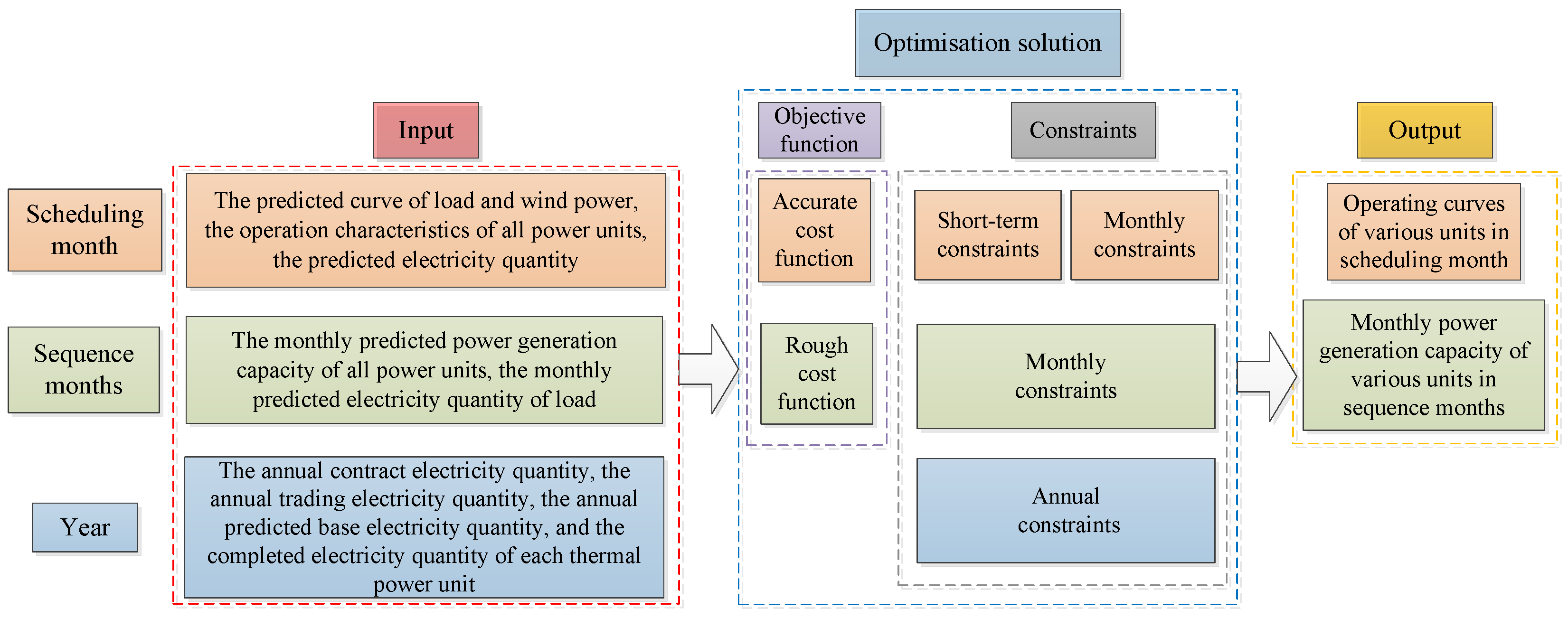
2. Modelling Concept and Method

As stated previously, methods such as average decomposition and the deviation of the load ratio cannot effectively solve the problem of formulating the monthly energy-trade scheduling, when the renewable energy is absorbed by the power grid on a large scale. However, the time-sequence simulation method is a dynamic optimization method simulated by setting up an objective function and the relevant constraints. It is characterized by both long-time and short-time scales. In the long-time scale, the optimal values at each time point can be accumulated and the sum can be macroscopically restricted by the fairness constraints. In the short time scale, the optimal solutions can be obtained considering the detailed operation constraints at each time interval. The time-sequence simulation method matches with the modelling demand of monthly energy-trade scheduling. Therefore, the time-sequence simulation method is very suitable for the modelling of the monthly energy-trade scheduling.

To improve the operation economy and utilization rate of renewable energy, the objective function of the model is to minimize the combined costs including the coal consumption cost, peaking cost, start-up and shutdown cost, hydropower abandoning cost, wind power curtailment cost, and nuclear power peak shaving cost in the remaining months. To better consider multiple factors during the actual power operation, the annual constraints, monthly constraints, and short-term constraints are all considered. In the annual constraints, the energy completion rate deviation constraints are introduced to meet the power generation fairness requirement. The monthly power energy balance constraints for each generation unit are considered in the monthly constraints, to ensure reasonable allocation of the monthly scheduling energy. Operation constraints including the generator characteristic constraints, power balance constraints, and spinning reserve constraints are considered in the hourly short-term constraints, to reduce the deviation between monthly scheduling and daily dispatching, and improve the schedule feasibility. According to the typical time-sequence simulation method, the monthly energy-trade scheduling problem is modelled and simulated on an hourly basis, from the beginning of the decision point to the end of the whole year. The detailed process is shown in Figure 1.

However, some problems are faced when using the typical time-sequence simulation method mentioned above in the modelling of monthly energy-trade scheduling.

• During the optimizing months, the method is optimized on an hourly basis. A system operation with up to 8760 time intervals must be simulated. For large-scale power systems with hundreds of generation units, such a demand presents a massive scale optimization problem, which is difficult to solve.
• Considering the low accuracy of long-term forecasting of wind power, water inflow, and the load, the simulation results in the months farther from the decision point might be vastly different from the actual operation, which may increase the wind and water curtailment level.

Therefore, it is neither necessary nor feasible to simulate the system operation in the whole period on an hourly basis. Some works in the literature proposed preliminary solutions to this problem. For example, Reference [26] proposed a segmented idea to simplify the calculation, but adopted the method of average segmentation throughout the process, which is too simplistic and does not conform to the physical characteristics of the accuracy of the predicted value decay with time. In another example, Reference [27] divided each day into three sections—peak, flat, and valley—which did not meet the law of change in prediction. Based on these ideas, a segment modelling strategy for the monthly energy-trade scheduling is presented. The system simulation is former-accurate and after-rough. The remaining months are decomposed into the scheduling month and the subsequent months. The scheduling month is the next month after the decision point, and the subsequent months include the months after the scheduling month to the end of the year. For the scheduling month, since the load forecast accuracy is higher and wind power forecasting data could be used, the system operation is still simulated hourly, and, thus, the cost function (defined as the accurate cost function), the monthly constraints, and the short-term constraints are the same as in the typical method introduced above. In addition, for the subsequent months, since the load forecast accuracy is lower and no wind power forecasting results could be used, the system operation is simulated monthly, and the cost function (defined as the rough cost function) only contains the coal consumption cost of thermal power units, to ensure the economy of the model, and only the monthly constraints are considered. The short-term constraints, which require the prediction data with high accuracy and large-scale calculation, are abandoned in the subsequent months. The electric energy completion situation in the completed month involves the formulation for the next month as an input. Additionally, it is constrained by the annual constraints with the electrical energy of the scheduling month and the subsequent months. The process is shown in Figure 2.

In the actual application, the monthly electrical energy-trade scheduling is rolling when scheduled from the start of the year to November of that year. During each decision period, the completed energy of each generation unit is applied to correct the energy target of the remaining months.

3. Mathematical Model

3.1. Objective Function

The objective function of the monthly energy-trade scheduling model is to minimize the sum of total costs for the remaining months. As mentioned above, to improve the feasibility of the model and the solving efficiency, the accurate cost function $F_1$ is used in the scheduling month, and the rough cost function $F_2$ is used in subsequent months.

$$\min F=\min (F_1+F_2)$$

(1)

3.1.1. Accurate Cost Function for the Scheduling Month

The accurate cost function for the scheduling month is the total costs of all the different types of units in the scheduling month, which consist of the operational costs of the condensing thermal power units and operational cost, the steam extraction thermal power units, the curtailment cost of the wind power units, the abandoning cost of the hydropower units, and the peak shaving cost of the nuclear power units.

$$F_1={\displaystyle \sum _{t=1}^T\left\{{\displaystyle \sum _{i=1}^{N_{CN}}{f}_{CN}(i,t)}+{\displaystyle \sum _{k=1}^{N_{CQ}}{f}_{CQ}(k,t)}+{\displaystyle \sum _{l=1}^{N_w}{f}_w(l,t)}+{\displaystyle \sum _{s=1}^{N_m}{f}_m(s,t)}+{\displaystyle \sum _{v=1}^{N_n}{f}_n(v,t)}\right\}}$$

(2)

The nomenclature of variables can be found in Appendix A.

The operation costs of the condensing thermal power units are composed of the coal consumption cost, deep-peak-regulation cost, and start-up and shut-down costs.

$$f_{CN}(i,t)=a_i{(P_{C{N}_i}^t)}^2+b_i(P_{C{N}_i}^t)+c_i+M\times \Delta P_{C{N}_i}^t+S_{C{N}_i}{u}_i^t(1-u_i^t)$$

(3)

The operation costs of the steam extraction thermal power units include the coal consumption cost, deep peak-regulation cost, and the start-up and shut-down costs.

$$\begin{array}{ll}{f}_{CQ}(k,t)& =a_k{(P_{C{Q}_k}^t+C_{v1}\times H_{C{Q}_k}^t)}^2+b_k(P_{C{Q}_k}^t+C_{v1}\times H_{C{Q}_k}^t)+c_k\\ & +M\times \Delta P_{C{Q}_k}^t+S_{C{Q}_k}{u}_k^t(1-u_k^t)\end{array}$$

(4)

The wind power curtailment cost is:

$$f_w(l,t)=C_w(P_{w_l}^t-\widetilde{P_{w_l}^t})$$

(5)

The hydropower abandoning cost is:

$$f_m(s,t)=C_m{P}_{m,g}^t$$

(6)

The nuclear power peak-regulation cost is:

$$f_n(v,t)=C_n(\stackrel{\_}{P_{n_v}}-P_{n_v}^t)$$

(7)

3.1.2. Rough Cost Function for Subsequent Months

The rough cost function is reduced to the sum costs of thermal units in the sequence months, including the condensing thermal power units and steam extraction thermal power units.

$$F_2={\displaystyle \sum _{e=m+1}^{12}({\displaystyle \sum _{i=1}^{N_{CN}}{W}_{C{N}_i,RE}^e\times }{C}_{C{N}_i}+{\displaystyle \sum _{k=1}^{N_{CQ}}{W}_{C{Q}_k,RE}^e\times C_{C{Q}_k})}}$$

(8)

3.2. Constraint Conditions

3.2.1. Short-Term Constraints

To ensure the feasibility of the monthly energy-trade scheduling, the short-term constraints limit the operation status of the units in each time interval of the scheduling month. The operation constraints of various units, and the power balance constraint and spinning reserve constraints are considered.

The short-term constraints of the condensing thermal power units include the maximum and minimum output constraints, ramp rate constraints, and minimum start-off time constraints. The constraints considered are as follows.

$$\{\begin{array}{l}{u}_i^t{P}_{C{N}_i,\min }^{}\le P_{C{N}_i}^t\le u_i^t{P}_{C{N}_i,\max }^{}\\ -\Delta P_{C{N}_i,down}^{}\le P_{C{N}_i}^t-P_{C{N}_i}^{t-1}\le \Delta P_{C{N}_i,up}^{}\\ (u_i^t-u_i^{t-1})(X_{C{N}_i,on}^{t-1}-T_{C{N}_i,on}^{})\le 0\\ (u_i^{t-1}-u_i^t)(X_{C{N}_i,off}^{t-1}-T_{C{N}_i,off}^{})\le 0\end{array}$$

(9)

The short-term constraints of the steam extraction thermal power units include the maximum and minimum output constraints, ramp rate constraints, minimum start-off time constraints, thermoelectric relationship constraint, reserve capacity constraint, and thermal balance constraint. The constraints considered are below.

$$\{\begin{array}{l}{u}_k^t{P}_{C{Q}_k,\min }^{}\le P_{C{Q}_k}^t\le u_k^t{P}_{C{Q}_k,\max }^{}\\ -\Delta P_{C{Q}_k,down}^{}\le P_{C{Q}_k}^t-P_{C{Q}_k}^{t-1}\le \Delta P_{C{Q}_k,up}^{}\\ (u_k^{t-1}-u_k^t)(X_{C{Q}_k,off}^{t-1}-T_{C{Q}_k,off}^{})\le 0\\ (u_k^t-u_k^{t-1})(X_{C{Q}_k,on}^{t-1}-T_{C{Q}_k,on}^{})\le 0\\ \max (C_{m_k}\times H_{C{Q}_k}^t+K_k,P_{C{Q}_k,\min }^{}-C_{v{2}_k}\times H_{C{Q}_k}^t)\le P_{C{Q}_k}^t\le P_{C{Q}_k,\max }^{}-C_{v{1}_k}\times H_{C{Q}_k}^t\\ 0\le H_{C{Q}_k}^t\le H_{C{Q}_k,\max }^{}\\ {\displaystyle \sum _{k=1}^{N_{CQ}}{H}_{C{Q}_k}^t}=H_L^t\end{array}$$

(10)

In the short-term constraints of wind turbines, the wind power output should be equal to or less than the forecasted wind power. The constraints considered are below.

$$0\le P_{w_l}^t\le \stackrel{\_}{P_{w_l}^t}$$

(11)

The short-term constraints of the hydropower units are composed of the upper and lower limits of the reserve capacity, the upper limit constraint of the water flow for generating power, and the maximum output constraint. The constraints considered are below.

$$\{\begin{array}{l}{V}_m^{t+1}=V_m^t+f_m^t-{\displaystyle \sum _{s=1}^{N_m}{q}_{m_s}^t}-g_m^t\\ V_m^{\min }\le V_{m_s}^t\le V_m^{\max }\\ 0\le q_{m_s}^t\le q_{m_s,\max }^{}\\ P_{m_s}^t=a{q}_{m_s}^{t}h\\ 0\le P_{m_s}^t\le \min \{P_{m_s,\max }^{},a{q}_{m_s}^t{h}_{m_s}^t\}\end{array}$$

(12)

The nuclear power units perform the 15-1-7-1 power generation mode, which means that the nuclear power units maintain the state of full power generation for 15 h, and then decrease to the state of low power generation within 1 h. Then the nuclear power units maintain the low power generation state for 7 h, and return to the full power generation state in 1 h. The constraints considered are below.

$$\{\begin{array}{l}{u}_{n_v,y_1}^t+u_{n_v,y_2}^t=1\\ P_{n_v,y_1}^t=P_{n_{v,}\max }^{}\times u_{n_v,y1}^t\\ P_{n_v,y_2}^t=\alpha P_{n_v\max }^{}\times u_{n_v,y_2}^t\\ P_{n_v}^t=\max \{P_{n_v,y_1}^t,P_{n_v,y_2}^t\}\end{array}$$

(13)

The power balance constraint of the system is:

$${\displaystyle \sum _{i=1}^{N_{CN}}{P}_{C{N}_i}^t}+{\displaystyle \sum _{k=1}^{N_{CQ}}{P}_{C{Q}_k}^t+}{\displaystyle \sum _{l=1}^{N_w}\stackrel{}{P_{w_l}^t}}+{\displaystyle \sum _{s=1}^{N_m}{P}_{m_s}^t}+{\displaystyle \sum _{v=1}^{N_n}{P}_{n_v}^t}=P_L^t$$

(14)

The up and down spinning reserve constraints of the system are:

$${\displaystyle \sum _{i=1}^{N_{CN}}{P}_{C{N}_i,\max }^t}+{\displaystyle \sum _{k=1}^{N_{CQ}}{P}_{C{Q}_k,\max }^t+}{\displaystyle \sum _{s=1}^{N_m}{P}_{m_s,\max }^t}+{\displaystyle \sum _{v=1}^{N_n}{P}_{n_v,\max }^t}\ge 1.05P_L^t-1.2P_w^t+0.5\beta P_w^t$$

(15)

$${\displaystyle \sum _{s=1}^{N_m}{P}_{m_s,\min }^t}+{\displaystyle \sum _{v=1}^{N_n}{P}_{n_v,\min }^t}\le 0.95P_L^t-0.8P_w^t-0.5\beta P_w^t$$

(16)

3.2.2. Monthly Constraints

The monthly constraints limit the monthly scheduled energy in the scheduling month and the subsequent months, to ensure that the energy allocated in each month can be used to reasonably formulate the daily dispatching. The constraints include the upper and lower limits of the monthly power generation energy of various units and the monthly electricity balance constraint.

The monthly operation rate of the units in the monthly constraints of the condensing thermal power units is defined as:

$$\frac{W_{C{N}_i}^{year}-W_{C{N}_i}^{ywc}}{T_{wwc}\times P_{C{N}_i,\max }\times \eta }\le {\delta }_{C{N}_i}^e\le \min (1,\frac{W_{C{N}_i}^{year}-W_{C{N}_i}^{ywc}}{T_{wwc}\times P_{C{N}_i,\min }})$$

(17)

Then, the upper and lower limit constraints of electrical energy of the condensing power units are as follows:

$$P_{C{N}_i,\min }^{}\times t^e\times {\delta }_{C{N}_i}^e\le W_{C{N}_i,RE}^e\le P_{C{N}_i,\max }^{}\times \eta \times t^e\times {\delta }_{C{N}_i}^e$$

(18)

The electrical energy balance constraints of the steam extraction thermal power units are:

$$\{\begin{array}{l}\frac{W_{C{Q}_k}^{year}-W_{C{Q}_k}^{ywc}}{T_{wwc}\times P_{C{Q}_k,\max }\times \eta }\le {\delta }_{C{Q}_k}^e\le \min (1,\frac{W_{C{Q}_k}^{year}-W_{C{Q}_k}^{ywc}}{T_{wwc}\times P_{C{Q}_k,\min }})\\ P_{C{Q}_k,\min }^{}\times t^e\times {\delta }_{C{Q}_k}^e\le W_{C{Q}_k,RE}^e\le P_{C{Q}_k,\max }^{}\times \eta \times t^e\times {\delta }_{C{Q}_k}^e\end{array}$$

(19)

The monthly electrical energy constraints of the wind turbine, hydropower unit, and nuclear power unit are:

$$0\le W_{w_l,RE}^e\le W_{w_l,F}^e$$

(20)

$$0\le W_{m_s,RE}^e\le W_{m_s,F}^e$$

(21)

$$0\le W_{n_v,RE}^e\le W_{n_v,F}^e$$

(22)

The balance constraint of the monthly electrical energy is:

$${\displaystyle \sum _{i=1}^{N_{CN}}{W}_{C{N}_i,RE}^e+}{\displaystyle \sum _{k=1}^{N_{CQ}}{W}_{C{Q}_k,RE}^e+}{\displaystyle \sum _{l=1}^{N_w}{W}_{w_l,RE}^e+}{\displaystyle \sum _{m=1}^{N_m}{W}_{m_l,RE}^e+}{\displaystyle \sum _{v=1}^{N_n}{W}_{n_v,RE}^e}=W_{L,RE}^e$$

(23)

3.2.3. Annual Constraints

The energy generated in the completed months, the scheduled energy in the scheduling month, and the scheduled energy in the subsequent months constitute the total annual energy of each thermal power unit.

$$W_{T_i,A}={\displaystyle \sum _{e=1}^{m-1}{W}_{{}^{{}_{T_i,H}}}^e+}{\displaystyle \sum _{t=1}^T{P}_{T_i}^t+{\displaystyle \sum _{e=m+1}^{12}{W}_{{}_{T_i,RE}}^e}},$$

(24)

where the electrical energy of the completed month is the input, and the amount of electricity in the scheduling month and the subsequent months is constrained by the annual fairness constraints as the optimization value. The deviation of electrical energy in the completed month can be corrected when formulating the monthly energy-trade scheduling.

The total annual energy of the thermal power units is composed of the annual base electrical energy and the annual transaction energy.

$$W_{T_i,A}=W_{T_i,B}+W_{T_i,D}$$

(25)

The annual transaction energy is composed of the tie-line energy, the generation right transfer trading energy, and the trading energy of large consumers.

$$W_{T_i,D}=W_{T_i,N}+W_{T_i,O}+W_{T_i,Y}$$

(26)

The completion rate of the annual base electrical energy of the total thermal power units, ${\rho }_T$ is defined as the ratio of the optimized annual base electrical energy of all thermal power units and the expected annual base electrical energy of all thermal power units.

$${\rho }_T=\frac{{\displaystyle \sum _{i=1}^{N_T}{W}_{T_i,B}}}{{\displaystyle \sum _{i=1}^{N_T}{W}_{T_i,BF}}}$$

(27)

According to the National Development and Reform Committee of China’s guide on strengthening and improving the regulation of power generation operation, the deviation threshold of the completion rate of the annual base electrical energy of each thermal unit is defined as $\lambda$%. The allocated fairness constraint for the annual base electrical energy of thermal power units is as follows:

$$(1-\lambda \%){\rho }_T\le \frac{W_{T_i,B}}{W_{T_i,BF}}\le (1+\lambda \%){\rho }_T$$

(28)

4. Simulation and Analysis

4.1. Simulation Condition

For the solving methods in this paper, since it is actually a large-scale mixed integer quadratic programming model, the Branch Bound (BB) methods, for instance, could be applied. In the case studies, we used the IBM CPLEX Business optimization software to solve the monthly energy-trade scheduling problem in the test system.

The test system consists of four condensing thermal power units, two steam-extraction thermal power units, one 600 MW hydropower station, one 250 MW wind farm, and one 60 MW nuclear power station. The simulation process of monthly energy-trade scheduling is shown in Figure 3.

April is assumed to be the scheduling month. The electrical energy and operation parameters and the operation cost coefficient of the thermal power units are shown in

Table 1. Electrical energy data of thermal power units.

Units	Annual Contract Electricity Quantity (MWh)	Annual Trading Electricity Quantity (MWh)	Annual Predicted Base Electricity Quantity (MWh)	The Completer Electricity Quantity in 1~3 Months (MWh)
1	3,139,000	2,511,200	627,800	876,740.1
2	1,569,500	1,255,600	313,900	452,014.1
3	1,307,900	1,046,320	261,580	322,918.3
4	784,800	627,840	156,960	197,038.9
5 (CHP)	1,689,800	1,351,840	337,960	441,868.7
6 (CHP)	1,109,100	887,280	221,820	325,208.2

,

Table 2. The operation parameters of thermal power units.

Units	Pmax (MW)	Pmin (MW)	Ton, min/Toff, min (h)	Pup (MW/h)	Pdown (MW/h)
1	600	280	8	168	168
2	350	140	5	80	80
3	250	100	5	80	80
4	150	70	6	42	42
5 (CHP)	323	150	6	90	90
6 (CHP)	212	100	6	60	60

and

Table 3. The operation cost coefficient of the thermal power units.

Units	S (¥/MWh)	A (¥/MW2h)	B (¥/MWh)	C (¥/h)	Average Coal Consumption Cost (¥/h)
1	1,200,000	0.06	157.8	6300	203.0
2	650,000	0.048	112.8	13,440	174.6
3	500,000	0.045	130.8	8640	182.8
4	260,000	0.04	164.4	3240	195.8
5 (CHP)	600,000	0.046	163.0	11,293	218.5
6 (CHP)	500,000	0.103	162.3	6922	221.4

, respectively. The thermoelectric relationship coefficient data of the thermoelectric units are shown in

Table 4. The thermoelectric relationship coefficient of thermoelectric units.

Units	Cv1	Cv2	Cm	K
5 (CHP)	0.23	0.23	0.45	80.7
6 (CHP)	0.21	0.21	0.45	45.4

. The characteristic parameters of the hydropower station and the reservoir are shown in

Table 5. The characteristic parameters of the hydropower station.

Unit	Pmax (MW)	qmax (m3/s)	a	Annual Contract Electricity Quantity (MWh)
1	600	705.9	8.5	2,607,169

and

Table 6. The characteristic parameters of the reservoir.

Reservoir	Vmax (m3)	Vmin (m3)	V0 (m3)	h (m)
1	90.18 × 108	40.09 × 108	60 × 108	100

, respectively. The monthly predicted hydropower electrical energy (PHEQ) is shown in

Table 7. The monthly predicted hydropower electrical energy.

Month	1	2	3	4	5	6
PHEQ (MWh)	44,847	81,109	102,817	138,739	174,379	300,159
Month	7	8	9	10	11	12
PHEQ (MWh)	359,829	429,932	350,262	307,388	161,367	156,341

. The characteristic parameters of the reservoir are shown in Table 6. The cost for deep-peak regulation is 500 ¥/MWh.

Load and wind power prediction methods have always been research interests in recent decades. A lot of research results have been obtained and many methods have been proposed. The widely used prediction methods include the Depth Ridgelet Neural Network method, support vector machine, etc. This paper focuses on the formulation of monthly energy-trade scheduling. Before it is formulated, the load and wind power forecasting results have been obtained by using existing prediction methods. Therefore, the load and wind power prediction methods are not the research contents of this paper. In the case studies, the predicted wind power electrical energy (PWEE) is randomly generated based on the historical wind power data. As shown in

Table 8. The monthly predicted wind-power electrical energy.

Month	1	2	3	4	5	6
PWEQ (MWh)	20,772	20,772	34,620	58,162	50,546	46,391
Month	7	8	9	10	11	12
PWEQ (MWh)	29,842	26,721	39,744	48,884	51,792	49,720

, the error range of monthly wind electricity energy prediction in Reference [28,29] was adopted for the calculation. The actual wind generation energy in April was 61,654 MWh, which was 6.04% deviation from the predicted wind power electric energy. The actual wind power generation curve is shown in Figure 4.

The annual load electrical energy is assumed to be 13.123323 × 10⁶ MWh and the monthly load coefficients are shown in

Table 9. The monthly load coefficients.

Month	1	2	3	4	5	6
Load coefficients	0.0949	0.0682	0.0702	0.0732	0.0752	0.0772
Month	7	8	9	10	11	12
Load coefficients	0.0992	0.0972	0.0912	0.0832	0.0722	0.0982

. The load curve in April (the scheduling month) is shown in Figure 5.

4.2. Simulation Results

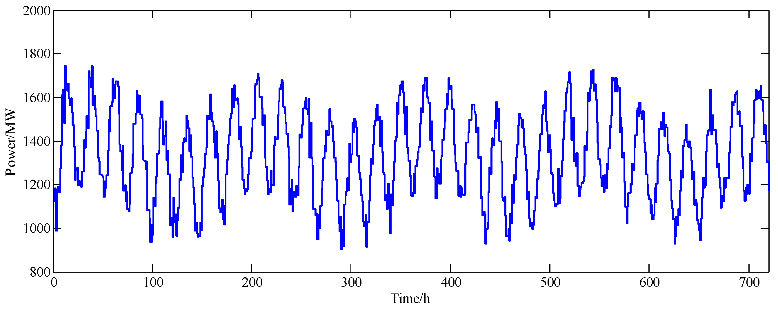
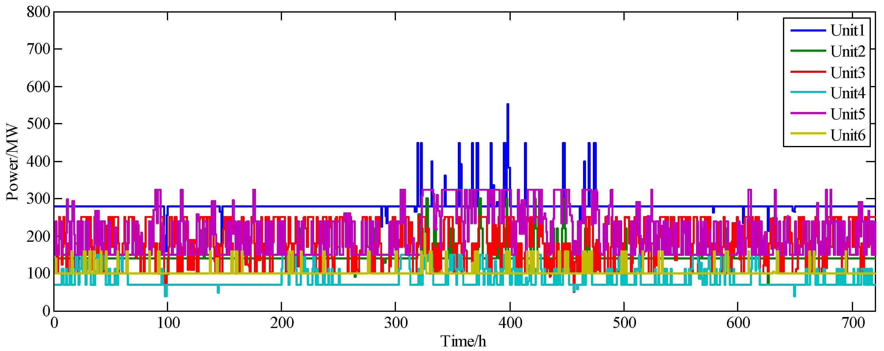
4.2.1. Simulation Results of April (the Scheduling Month)

1. Computational Performance Analysis

To verify the computational performance of the proposed approach, a simplified test system only including the thermal power units was simulated with simple constraints. The running time of the simplified traditional model on an hourly simulation was 1024.92 s. The optimization of the traditional model did not converge because the calculation amount was excessive. However, the computational time using the proposed approach and model was 28.15 s. The computational speed was increased by 97.25%, and the computational volume was reduced effectively. The convergence of optimizing could be ensured when applying the proposed method and model.

2. Economy, Energy Conservation, and Emission Reduction Effect Analysis

The monthly scheduled energy of the thermal power units from April to December, according to the proposed method, are shown in

Table 10. The scheduled energy of thermal power units using the proposed method.

Units	Month
	4	5	6	7	8	9	10	11	12
1	206,840.2	204,913.7	143,514.6	148,298.4	357,120.0	345,600.0	344,914.7	187,073.0	316,955.0
2	102,170.2	63,372.9	182,371.2	208,320.0	63,372.9	67,450.3	63,372.9	201,600.0	172,327.0
3	87,763.6	55,116.8	139,164.2	148,800.0	55,116.8	144,000.0	55,116.8	144,000.0	148,800.0
4	63,404.6	89,280.0	37,705.2	60,493.8	89,280.0	86,400.0	38,962.1	37,705.2	89,280.0
5 (CHP)	177,520.1	185,531.3	77,667.0	192,249.6	165,640.7	77,667.0	80,255.9	77,667.0	192,249.6
6 (CHP)	88,819.6	126,182.4	49,856.7	117,176.2	51,518.6	49,856.7	115,656.6	49,856.7	126,182.4

. For comparison, the monthly scheduled energy values of the thermal power units, according to the load rate deviation method, are shown in

Table 11. The scheduled energy of thermal power units using the load rate deviation method.

Units	Month
	4	5	6	7	8	9	10	11	12
1	235,580.1	243,661.8	205,164.9	294,433.0	263,053.9	250,963.2	234,876.6	227,177.2	351,768.5
2	120,967.0	120,210.3	101,217.9	145,258.2	129,777.4	123,812.4	115,876.1	112,077.6	173,544.6
3	105,224.8	104,566.5	88,045.8	126,354.8	112,888.6	107,699.9	100,796.4	97,492.2	150,960.1
4	67,181.1	63,367.4	53,355.8	76,571.2	68,410.6	65,266.3	61,082.7	59,080.4	91,482.0
5 (CHP)	128,855.4	133,275.8	112,219.2	161,046.2	143,882.7	137,269.5	128,470.6	124,259.3	192,407.0
6 (CHP)	81,473.6	84,268.5	70,954.7	101,827.4	90,975.1	86,793.7	81,230.2	78,567.5	121,656.4

.

The thermal power generation cost was calculated according to the average coal consumption cost coefficient in Table 3. During the period from April to December, the thermal power generation costs, according to the proposed method and the load rate deviation method, were ¥ 1,388,520,214.3 (¥ 1.388 billion) ¥ and ¥ 1,397,646,068.9 (¥ 1.397 billion), respectively. Compared with the load rate deviation method, the proposed method could save ¥ 9,125,854.6 (¥9.126 million).

The total scheduled energy values of thermal power units in the scheduling month were 61,654.1 MWh when the presented time-sequence simulation method was applied in the simulation and 58,162.0 MWh when the load rate deviation method was applied. The energy of renewable energy units generated by the time-sequence simulation method and the benefits of energy conservation and emission reduction were verified.

If the operating cost of various types of units, the deep peak-regulation cost, and the start-up cost of thermal power units were considered in the scheduling month, then the total comprehensive generation cost from April to December with the time-sequence simulation method was ¥ 1,389,168,214.3 (or ¥ 1.389 billion).

3. Feasibility Analysis

The hourly power output curve of each thermal power unit in April (the scheduling month), according to the presented method is shown in Figure 6. The hourly output of each power unit in the scheduling month with the time-sequence simulation method can be obtained under the premise that the reliability of the generator and system operation is guaranteed. With the time-sequence simulation method, all the constraints together could ensure that the power output of each power unit is close to the actual operating conditions, which means a higher feasibility could be ensured.

4. Fairness Analysis

The monthly energy-trade scheduling is simulated, according to the presented method, when considering the completed rate thresholds (CRTs) for different annual base electrical energies. The total costs based on different CRTs are shown in

Table 12. Total cost based on different CRTs.

CRT	The Total Cost (¥)
2%	1,389,737,549.8
3%	1,389,168,214.3
5%	1,389,087,840.1
7%	1,388,881,156.7
10%	1,387,398,273.3

.

From Table 12, it can be seen that the relationship between the total cost and CRT are negatively correlated. With the increase in CRT, the relative optimization space of the monthly energy-trade scheduling became larger, so that there could be a more economical way to revise the monthly energy-trade scheduling. However, due to the increase in CRT, the fairness of generation scheduling was weaker. Therefore, the contradiction between the power generation units and the dispatching department was sharper. According to the current national regulations in China, the CRT was set to 3%. With the gradual improvement of market mechanism for electricity, the CRT could be adjusted more reasonably, according to the proportion of fairness and economy of the monthly energy-trade scheduling.

4.2.2. Rolling Correction Results during the Whole Year

The scheduling month was moved from January to December. The monthly energy-trade scheduling results for the whole year after the rolling correction are shown in

Table 13. The monthly energy-trade scheduling results for the whole year.

Units		Month
		1	2	3	4	5	6
Thermal Power plants	1	387,134.0	242,411.3	247,194.7	206,840.2	232,986.9	202,367.6
	2	198,550.9	131,918.9	121,544.3	102,170.2	140,135.5	101,553.7
	3	148,287.9	90,969.3	83,661.1	87,763.6	92,291.6	74,537.9
	4	80,500.3	58,160.3	58,378.4	63,404.6	56,976.4	57,423.3
	5 (CHP)	198,032.3	122,431.6	121,404.8	177,520.1	122,722.2	112,861.3
	6 (CHP)	118,291.4	100,518.6	106,398.2	88,819.6	78,201.0	75,727.2
Wind unit		36,659.6	32,809.7	46,058.9	61,654.1	56,428.5	54,982.0
Hydropower station		44,847.0	81,109.0	102,817.0	138,739.0	174,379.0	300,159.0
Nuclear plant		37,200.0	33,600.0	37,200.0	36,000.0	37,200.0	36,000.0
Units		Month
		7	8	9	10	11	12
Thermal Power plants	1	280,140.4	248,503.1	232,828.2	217,412.6	248,327.6	357,120.0
	2	151,354.0	117,253.8	108,857.5	114,130.4	73,712.6	205,244.2
	3	109,850.7	85,535.5	95,751.3	113,900.4	122,991.0	148,800.0
	4	71,886.7	64,416.1	57,709.4	53,655.8	64,151.3	89,280.0
	5 (CHP)	150,314.1	154,141.0	163,445.3	122,121.1	108,187.5	163,484.7
	6 (CHP)	102,852.1	104,726.4	107,678.0	76,745.4	79,663.5	81,865.1
Wind unit		42,685.4	40,271.0	48,806.3	52,327.0	57,692.1	49,720.0
Hydropower station		359,829.0	429,932.0	350,262.0	307,388.0	161,367.0	156,341.0
Nuclear plant		37,200.0	37,200.0	36,000.0	37,200.0	36,000.0	37,200.0

.

5. Conclusions

A new time-sequence simulation method for monthly energy-trade scheduling is presented in this paper. The feasibility of the presented method is validated at the theoretical level using a case study. The segment modeling strategy is applied to simulate on an hourly basis for the scheduling month and for the sequence months on a monthly basis. In the power systems integrated with large-scale new energy power, multiple factors such as the generation coordinate among various types of power units, equitable distribution of electrical energy, and system operation reliability could be comprehensively considered in the monthly energy-trade scheduling process.

The results of the case study verified the feasibility and effectiveness of the proposed approach.

• The characteristics of wind power, nuclear power, hydropower, thermal power, and combined heat and power (CHP) generators were comprehensively considered. Therefore, the consumption capability of renewable energy power can be improved, according to the presented monthly energy-trade scheduling method. Thus, the energy saving and emission reduction benefits can be improved.
• By efficiently managing the balance of the annual base electrical energy completion rate of each thermal power unit, the monthly energy trade scheduling fairness can be ensured in a better way.
• Because the necessary operating constraints in the short-term time-scale could be easily introduced into the mathematical model for the scheduling month, the feasibility of the monthly energy-trade scheduling could be improved significantly. This improvement can lay a good foundation for daily dispatching.

The limitation of this study is that it does not involve an experimental study. Therefore, in future studies, this method might need to be modified according to the actual operating conditions. These conditions may be the number of power plants in a regional power grid, calculation time limit, etc., which may improve the practicality of the proposed method.

References

1. Han, J.H. The Formulation Method of Annual Contract Energy Planning for Power Generation Unit under the Constraint of Energy Saving and Emission Reduction. Master’s Thesis, Harbin Institute of Technology, Harbin, China, 2011. [Google Scholar]
2. Tang, W. Research on the Method of Compiling Monthly Energy Trade Scheduling. Ph.D. Thesis, Harbin Institute of Technology, Harbin, China, 2009. [Google Scholar]
3. Zhang, H.Q.; Chang, Y.J.; Tang, D.Y.; Wang, S.Y.; Chen, Q.; Li, Z.G.; Wang, Y.Q.; Yu, J.L. A monthly electric energy plan making method of thermal power generation unit in Energy-Saving generation dispatching mode. Power Syst. Prot. Control 2011, 39, 84–89. [Google Scholar] [CrossRef]
4. Xia, Q.; Chen, Y.G.; Chen, L. Energy-Saving power generation scheduling mode and method considering monthly unit combination. Power Syst. Technol. 2011, 6, 27–33. [Google Scholar] [CrossRef]
5. Wang, Y.; Tang, W.; Luo, H.H.; Yu, F.; Liu, Z.Y.; Jin, Z.H.; Liu, J.; Guo, Y.F.; Yu, J.L.; Liu, Z. Load Rate Deviation Method for Preparing Monthly Energy Trade Scheduling for Thermal Power Generation Units. Power Syst. Prot. Control 2009, 22, 134–140. [Google Scholar] [CrossRef]
6. Tang, W.; Wang, Y.; Yu, F.; Liu, Z.Y.; Luo, H.H.; Jin, Z.H.; Liu, J.; Guo, Y.F.; Yu, J.L.; Liu, Z. Comprehensive Cost-weighting Method for Preparing Monthly Energy Trade Scheduling for Thermal Power Units. Power Syst. Technol. 2009, 33, 167–173. [Google Scholar] [CrossRef]
7. Tang, W.; Wang, Y.; Yu, J.L.; Min, D.J.; Luo, H.H.; Guo, Y.F.; Jin, Z.H.; Liu, J.; Liu, Z. Comprehensive Consumption Optimization Method for Preparing Monthly energy trade scheduling for Thermal Power Units. Proc. CSEE 2009, 29, 64–70. [Google Scholar] [CrossRef]
8. Mohammad, A.M.; Ahmad, S.Y.; Behnam, M.; Mousa, M.; Miadreza, S.-K.; Catalão, J.P.S. Stochastic network-constrained Co-Optimization of energy and reserve products in renewable energy integrated power and gas networks with energy storage system. J. Clean. Prod. 2019, 223, 747–758. [Google Scholar] [CrossRef]
9. Mousa, M.; Hamed, A.; Seyedeh, S.G.; Hasan, U.; Terrence, F. Optimal energy management system based on stochastic approach fora home Microgrid with integrated responsive load demand and energy storage. Sustain. Cities Soc. 2017, 28, 256–264. [Google Scholar] [CrossRef]
10. Korkas, C.D.; Baldi, S.; Michailidis, L.; Kosmatopoulos, E.B. Occupancy-based demand response and thermal comfort optimization in microgrids with renewable energy sources and energy storage. Appl. Energy 2016, 163, 93–104. [Google Scholar] [CrossRef]
11. Korkas, C.D.; Baldi, S.; Michailidis, L.; Kosmatopoulos, E.B. Intelligent energy and thermal comfort management in grid-connected microgrids with heterogeneous occupancy schedule. Appl. Energy 2015, 149, 194–203. [Google Scholar] [CrossRef]
12. Yu, J.; Ji, F.; Zhang, L.; Chen, Y.S. An over painted oriental arts: Evaluation of the development of the Chinese renewable energy market using the wind power market as a model. Energy Policy 2009, 37, 5221–5225. [Google Scholar] [CrossRef]
13. Chen, Q.; Fan-Chao, G.U.; Jin, Y.Q.; Qin, C.; Chen, X.Y.; Li, Z.R. Energy-Saving Generation Dispatch of Power System Including Large-scale Wind Farms. Proc. CSU-EPSA 2014. [Google Scholar] [CrossRef]
14. Chi, Y.N.; Liu, Y.H.; Wang, W.S.; Chen, M.Z.; Dai, H.Z. Study on Impact of Wind Power Integration on Power System. Power Syst. Technol. 2007, 31, 77–81. [Google Scholar] [CrossRef]
15. Rao, P.; Peng, C.H. A Research on Power Dispatch of Energy-saving and Emission-reduction Generation Based on the Improved Differential Evolution Algorithm. J. East China Jiaotong Univ. 2010, 2010. [Google Scholar] [CrossRef]
16. Ting, L.I.; Zhang, H.L.; Shao, P.; Guo, S.Q.; Guang, H.H. Economic evaluation method of monthly power generation plan considering the direct power purchase’ influence. Technol. Dev. Enterp. 2016. [Google Scholar] [CrossRef]
17. Wei, X.H.; Hu, Z.Y.; Yang, L. Thoughts and Suggestions about The Current Evaluation Indicators of the San Gong Dispatching. Autom. Electr. Power Syst. 2012, 36, 109–112. [Google Scholar] [CrossRef]
18. Tian, K.; Yao, J.; Wenhui, L.I. Power System Optimal Dispatching Model with Low-Carbon under Clean Energy Generation Integration. Shaanxi Electr. Power 2016. [Google Scholar] [CrossRef]
19. Zhong, H.; Xia, Q.; Chen, Y.; Kang, C.Q. Energy-Saving generation dispatch toward a sustainable electric power industry in China. Energy Policy 2015, 83, 14–25. [Google Scholar] [CrossRef]
20. Lin, R.M.; Jin, H.G.; Cai, R.X. Researching Direction and Development for New Generation Energy Power System. Power Eng. 2003. [Google Scholar] [CrossRef]
21. Liu, C.; Cao, Y.; Huang, Y.H.; Li, P.; Sun, Y.; Yuan, Y. The Method for Preparing Annual Wind Power Wind Power Plan Based on Time Series Simulation. Autom. Electr. Power Syst. 2014, 38, 13–19. [Google Scholar] [CrossRef]
22. Cao, Y.; Li, P.; Yuan, Y.; Zhang, X.S.; Guo, S.Q.; Zhang, C.F. New Energy Consumption Capacity Analysis and Low Carbon Benefit Evaluation Based on Time Series Simulation. Autom. Electr. Power Syst. 2014, 38, 60–66. [Google Scholar] [CrossRef]
23. Bai, L.P. The Economic Constraints and Economic Dispatch of Power Systems Considering New Energy Sources. Master’s Thesis, Harbin Engineering University, Harbin, China, 2016. [Google Scholar]
24. Ji, F.; Cai, X.G. Monthly unit combination model with wind power system. J. Harbin Inst. Technol. 2017, 3. [Google Scholar] [CrossRef]
25. Sun, L.; Xu, J.; Zhang, Q.; Shen, J.K.; Liu, X.L.; Li, W.D. A time sequential simulation method for monthly energy trade planning in the power system with multiple energy resources. J. Phys. Conf. Ser. IOP Publ. 2018, 1053, 012008. [Google Scholar] [CrossRef]
26. Li, X. Research on Optimization Method of Power System Monthly Power Purchase Scheduling. Master’s Thesis, Chongqing University, Chongqing, China, 2013. [Google Scholar]
27. Liang, Z.F.; Xia, Q.; Xu, H.Q.; Zhu, M.X.; Zhang, J.; Yang, M.H. Provincial grid monthly power generation plan based on multi-objective optimization model. Power Syst. Technol. 2009, 13, 90–95. [Google Scholar] [CrossRef]
28. Zhang, X.Q.; Bai, X.; Wan, Y.Z.; Peng, M.Q.; Wang, P.; Xiang, Y. Application of Grey Model in Wind Power Generation Forecast of Northwest Power Grid. Power Syst. Clean Energy 2011, 4, 66–70. [Google Scholar] [CrossRef]
29. Guo, D. Research on High Proportion of Wind Power Grid-Connected to Improve Consumption Capacity. Ph.D. Thesis, Shenyang Agricultural University, Shenyang, China, 2017. [Google Scholar]
Figure 1. The monthly energy-trade scheduling model according to the typical time-sequence simulation.
Processes 07 00771 g001
Figure 2. The monthly energy-trade scheduling model according to the improved time series simulation.
Processes 07 00771 g002
Figure 3. Simulation process of the monthly energy-trade scheduling.
Processes 07 00771 g003
Figure 4. The actual wind power generation curve.
Processes 07 00771 g004
Figure 5. The load curve in April.
Processes 07 00771 g005
Figure 6. The hourly power output curve of each thermal power unit in April.
Processes 07 00771 g006