Effects of a Dynamic Injection Flow Rate on Slug Generation in a Cross-Junction Square Microchannel


Abstract
1. Introduction
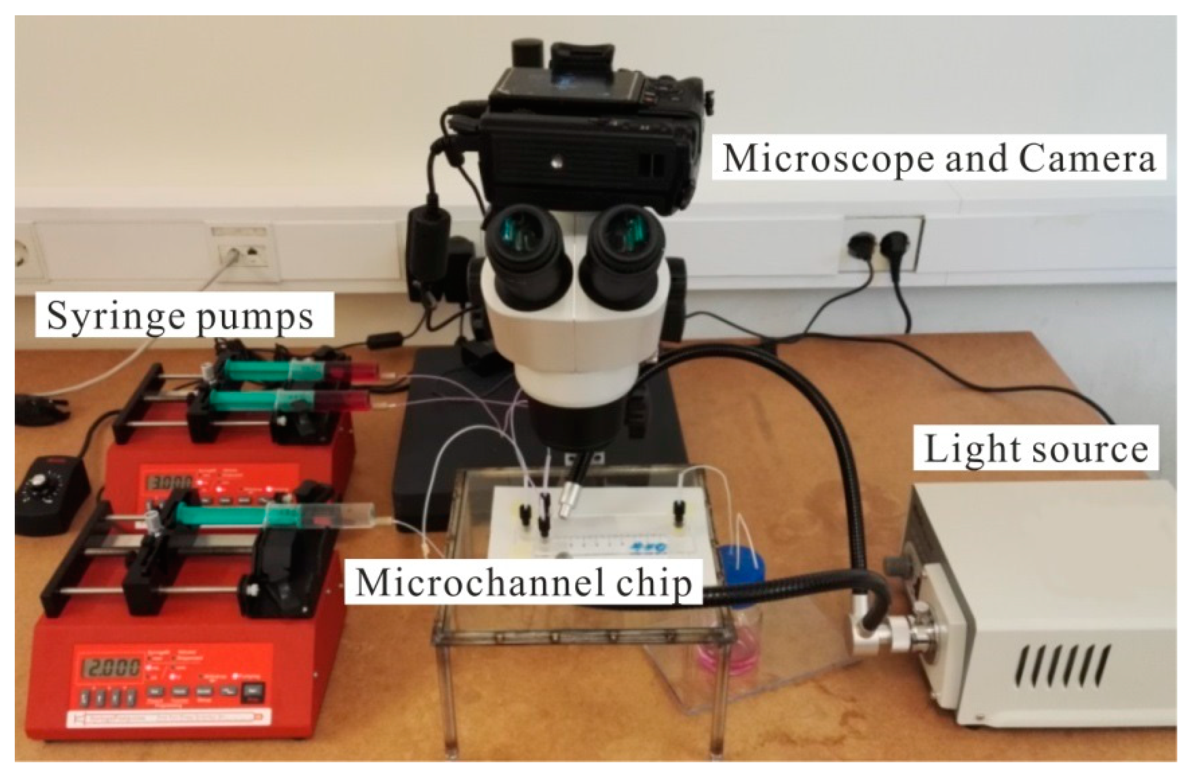
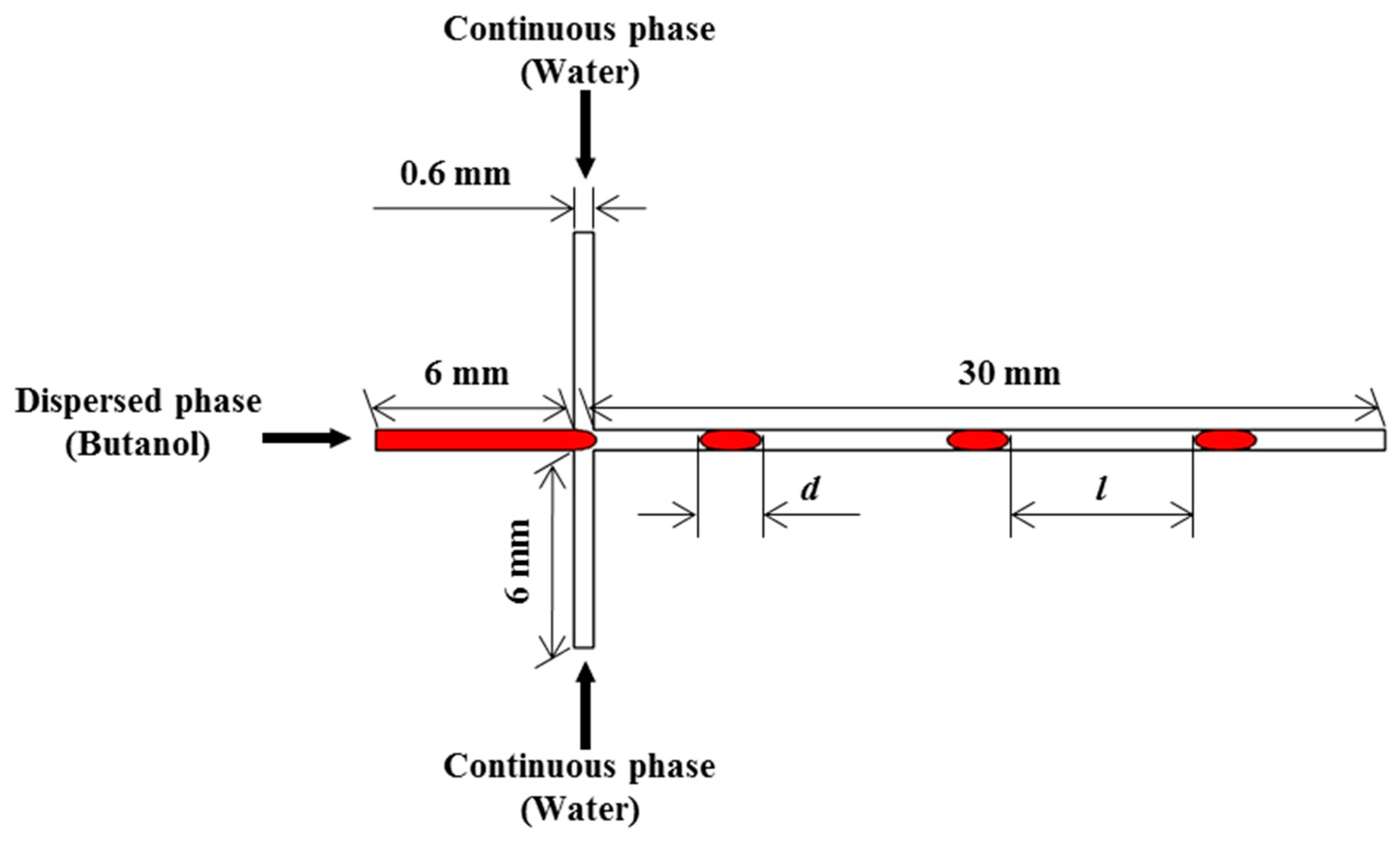
2. Experimental Setup
3. Numerical Method
3.1. Mathematical Model
3.2. Mesh and Boundary Conditions
4. Results and Discussion
4.1. Numerical Method Validation
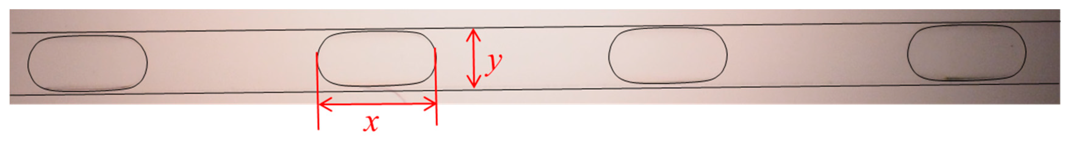
4.1.1. Experimental Results
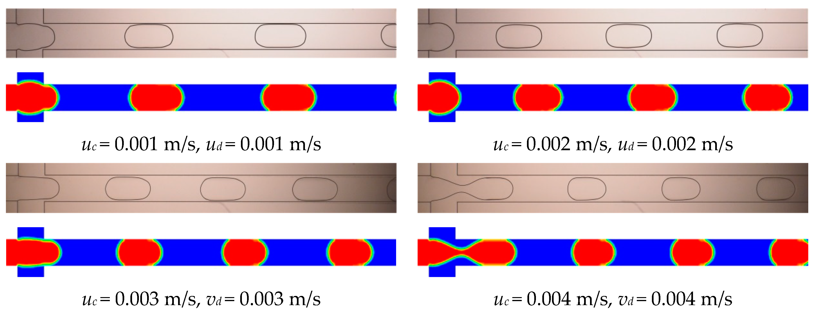
4.1.2. Validation of Numerical Method
4.2. Numerical Simulation Results of Dynamic Dispersed Injection Flow Rate
4.2.1. Comparison of Constant and Dynamic Injection Flow Rates
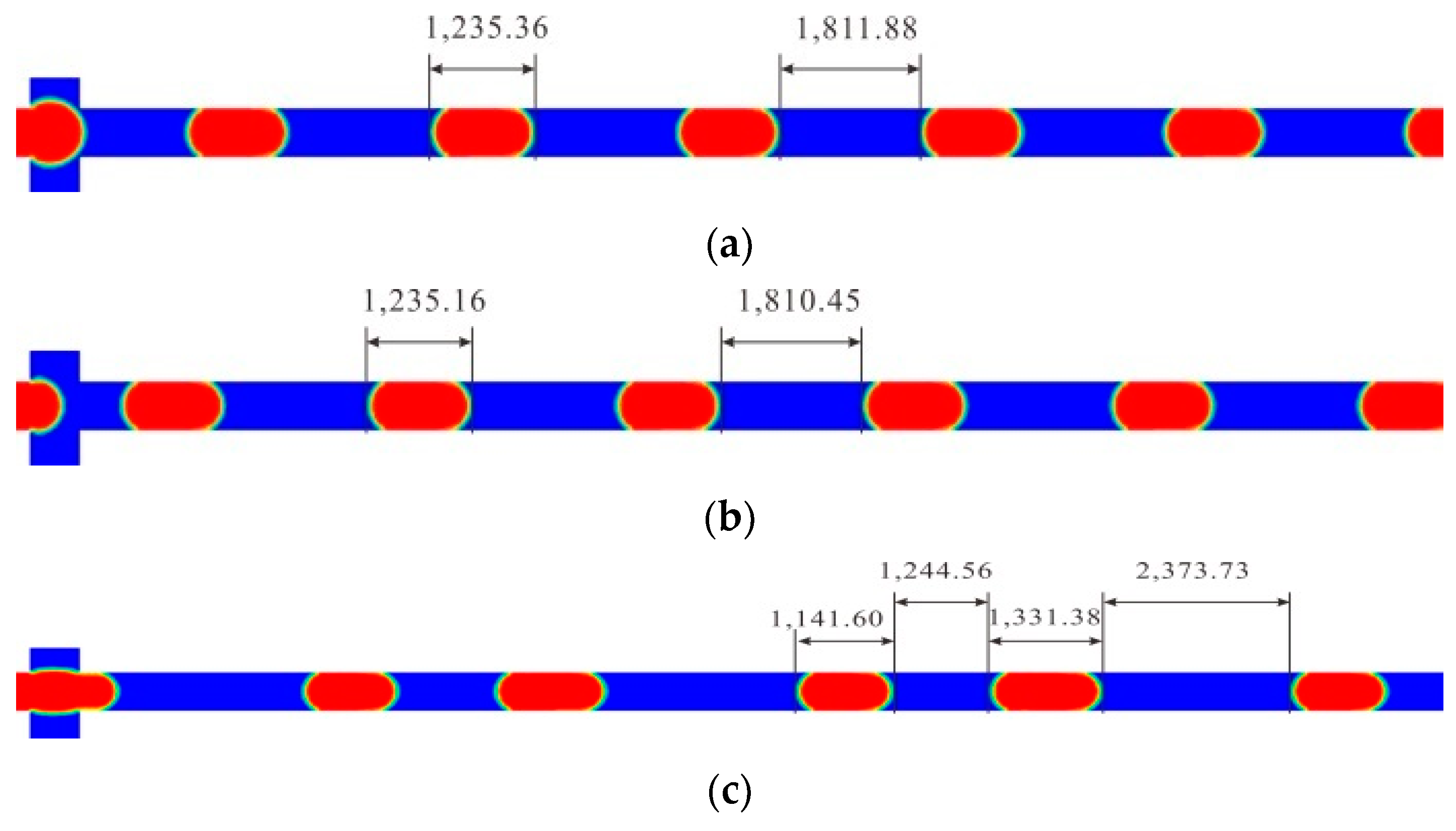
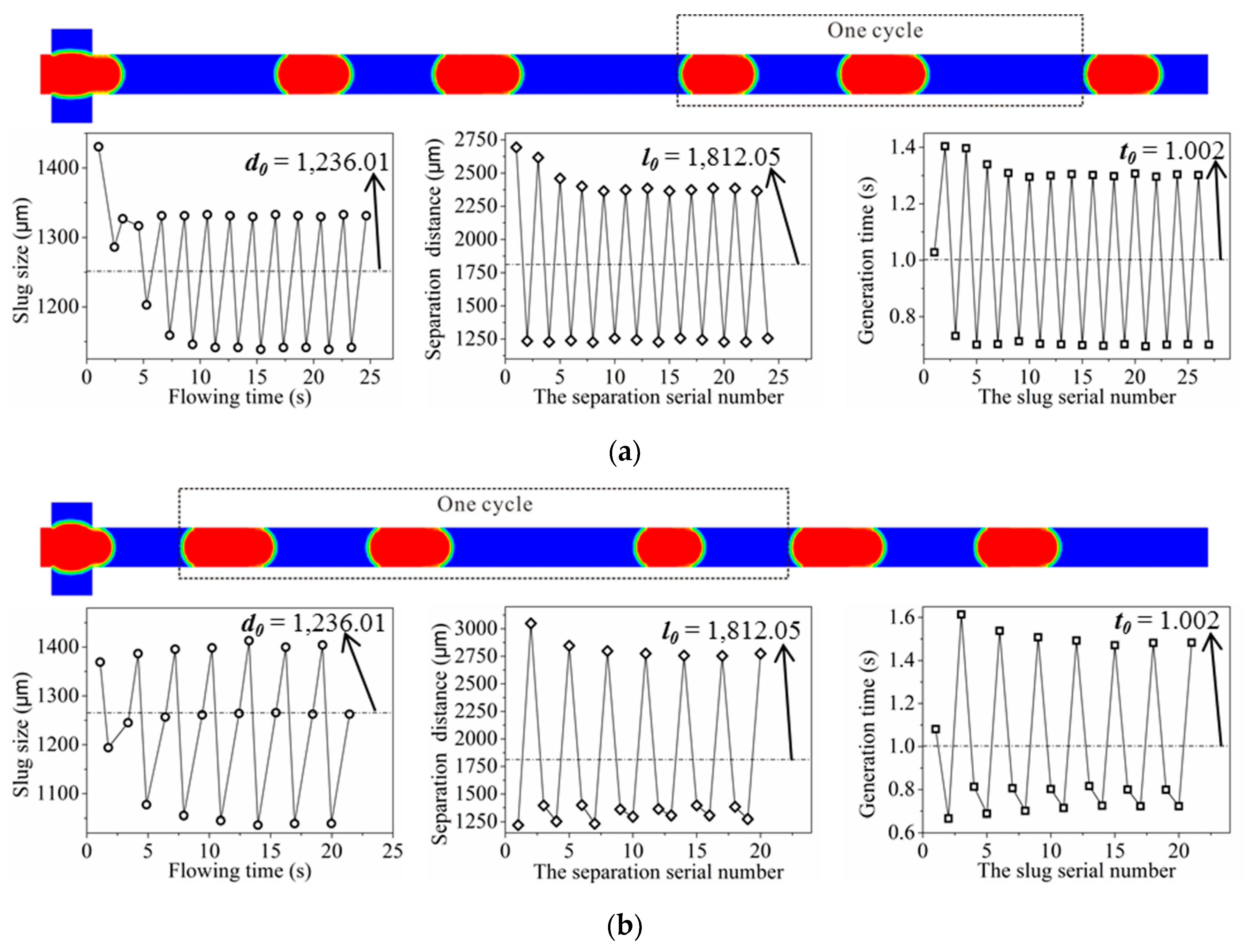
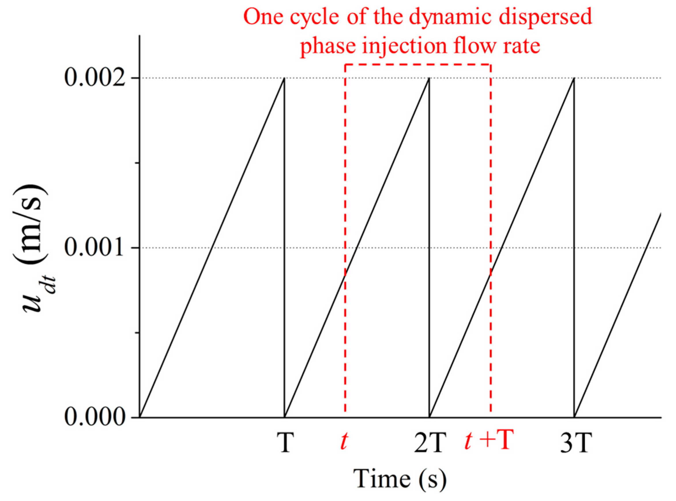
4.2.2. Cycle of the Dynamic Injection Flow Rate
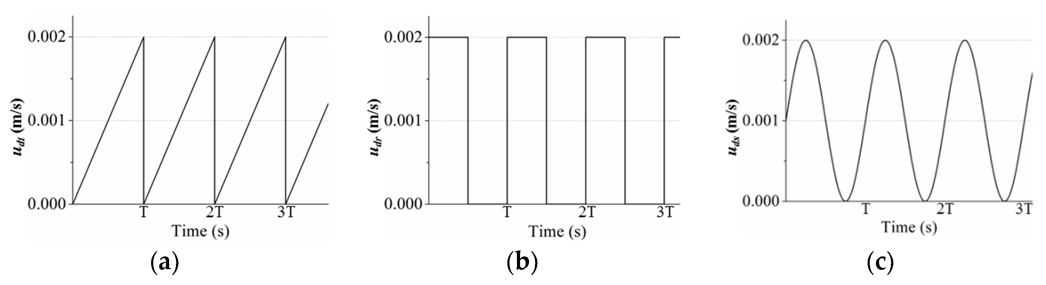
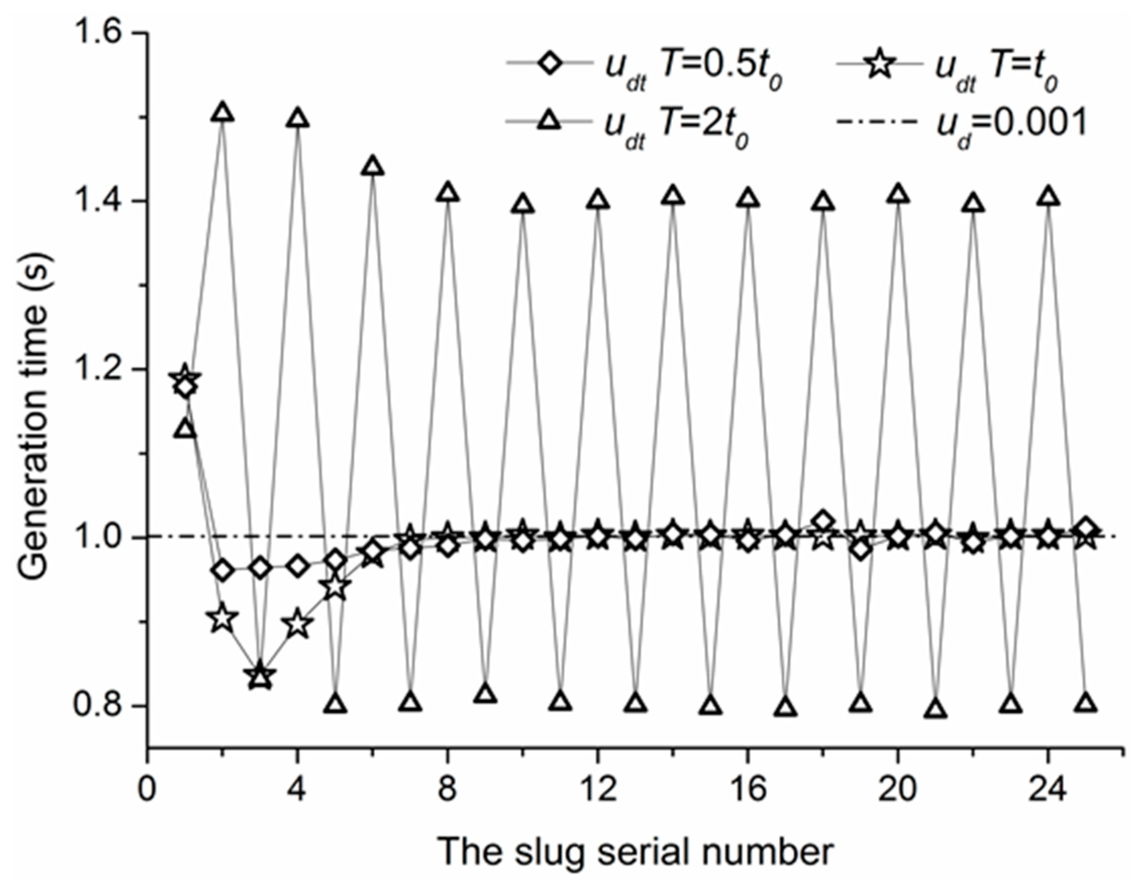
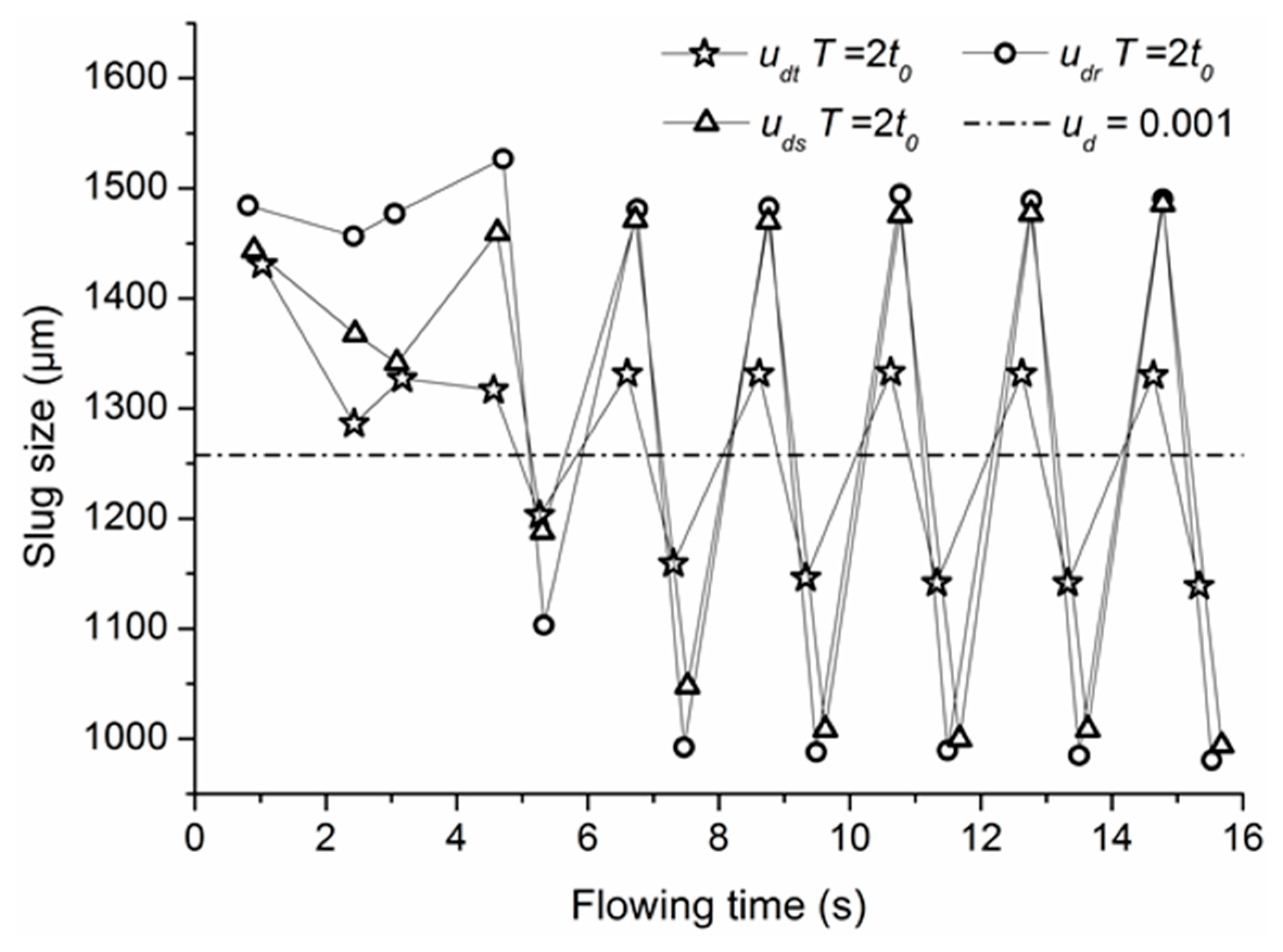
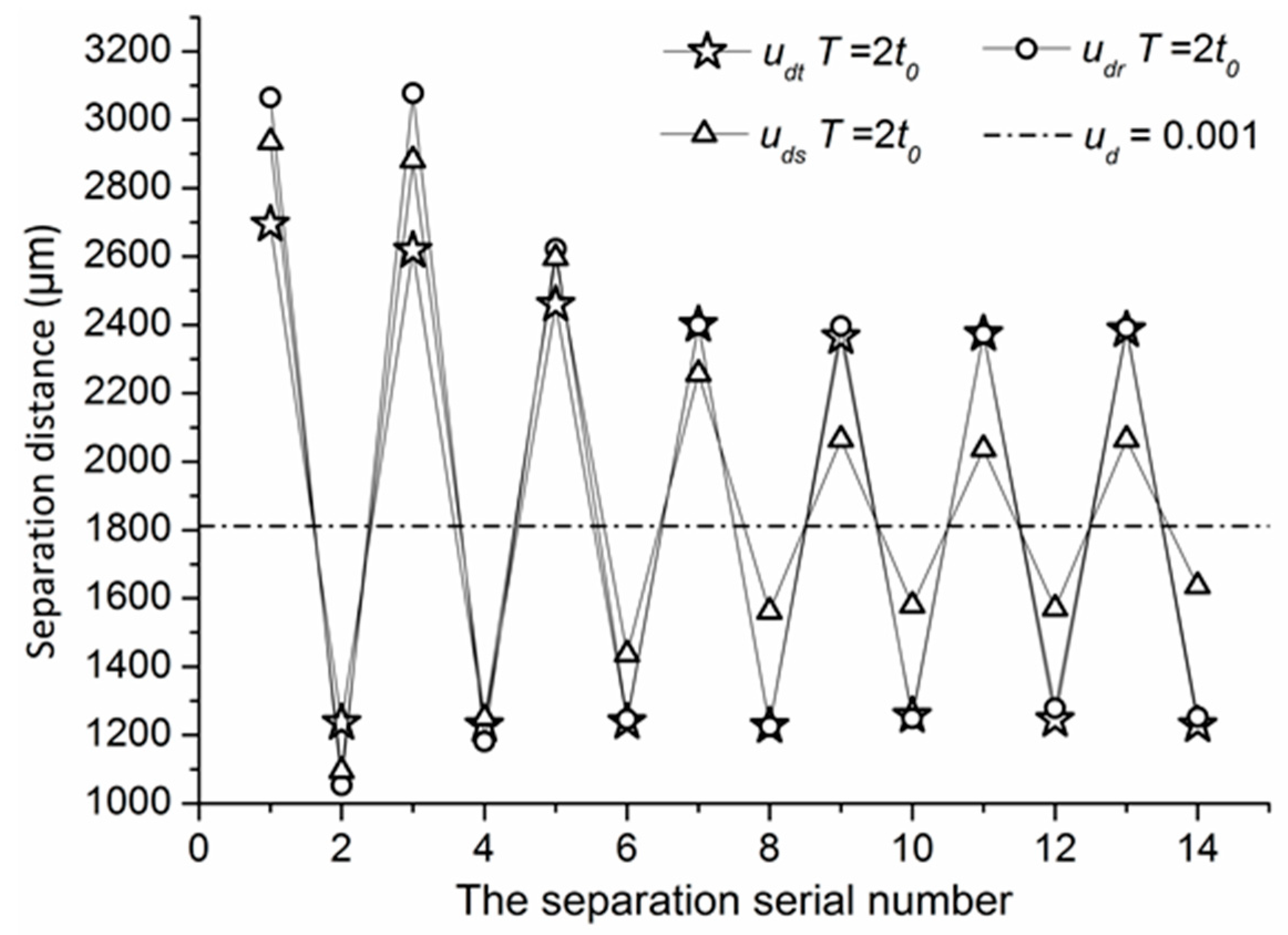
4.2.3. Different Types of the Dynamic Injection Flow Rate
5. Conclusions
Author Contributions
Funding
Conflicts of Interest
References
- Maan, A.A.; Nazir, A.; Khan, M.K.I.; Boom, R.; Schroën, K. Microfluidic emulsification in food processing. J. Food Eng. 2015, 147, 1–7. [Google Scholar] [CrossRef]
- Qian, J.; Li, X.; Wu, Z.; Bengt, S. A comprehensive review on liquid–liquid two-phase flow in microchannel: Flow pattern and mass transfer. Microfluid. Nanofluidics 2019, 23, 116. [Google Scholar] [CrossRef]
- Kurimoto, R.; Nakazawa, K.; Minagawa, H.; Yasuda, T. Prediction models of void fraction and pressure drop for gas-liquid slug flow in microchannels. Exp. Therm. Fluid Sci. 2017, 88, 124–133. [Google Scholar] [CrossRef]
- Liu, D.; Ling, X.; Peng, H. Experimental and numerical studies on microbubble generation and flow behavior in a microchannel with double flow junctions. Ind. Eng. Chem. Res. 2016, 55, 12276–12286. [Google Scholar] [CrossRef]
- Patel, R.S.; Weibel, J.A.; Garimella, S.V. Characterization of liquid film thickness in slug-regime microchannel flows. Int. J. Heat Mass Transf. 2017, 115, 1137–1143. [Google Scholar] [CrossRef]
- Rocha, L.A.M.; Miranda, J.M.; Campos, J.B.L.M. Wide range simulation study of taylor bubbles in circular milli and microchannels. Micromachines 2017, 8, 154. [Google Scholar] [CrossRef]
- Kingston, T.A.; Weibel, J.A.; Garimella, S.V. An experimental method for controlled generation and characterization of microchannel slug flow boiling. Int. J. Heat Mass Transf. 2017, 106, 619–628. [Google Scholar] [CrossRef][Green Version]
- Svetlov, S.D.; Abiev, R.S. Formation mechanisms and lengths of the bubbles and liquid slugs in a coaxial-spherical micro mixer in Taylor flow regime. Chem. Eng. J. 2018, 354, 269–284. [Google Scholar] [CrossRef]
- Yao, C.; Dong, Z.; Zhao, Y.; Chen, G. An online method to measure mass transfer of slug flow in a microchannel. Chem. Eng. Sci. 2014, 112, 15–24. [Google Scholar] [CrossRef]
- Yao, C.; Dong, Z.; Zhao, Y.; Chen, G. The effect of system pressure on gas-liquid slug flow in a microchannel. AIChE J. 2014, 60, 1132–1142. [Google Scholar] [CrossRef]
- Yao, C.; Liu, Y.; Zhao, S.; Dong, Z.; Chen, G. Bubble/droplet formation and mass transfer during gas–liquid–liquid segmented flow with soluble gas in a microchannel. AIChE J. 2017, 63, 1727–1739. [Google Scholar] [CrossRef]
- Yin, Y.; Zhu, C.; Guo, R.; Fu, T.; Ma, Y. Gas-liquid two-phase flow in a square microchannel with chemical mass transfer: Flow pattern, void fraction and frictional pressure drop. Int. J. Heat Mass. Transf. 2018, 127, 484–496. [Google Scholar] [CrossRef]
- Liu, Q.; Wang, W.; Palm, B. A numerical study of the transition from slug to annular flow in micro-channel convective boiling. Appl. Therm. Eng. 2017, 112, 73–81. [Google Scholar] [CrossRef]
- Magnini, M.; Thome, J.R. A CFD study of the parameters influencing heat transfer in microchannel slug flow boiling. Int. J. Therm. Sci. 2016, 110, 119–136. [Google Scholar] [CrossRef]
- Magnini, M.; Thome, J.R. An updated three-zone heat transfer model for slug flow boiling in microchannels. Int. J. Multiphase Flow 2017, 91, 296–314. [Google Scholar] [CrossRef]
- Li, H.; Hrnjak, P. Flow visualization of R32 in parallel-port microchannel tube. Int. J. Heat Mass Transf. 2019, 128, 1–11. [Google Scholar] [CrossRef]
- Garstecki, P.; Fuerstman, M.J.; Stonec, H.A.; Whitesides, G.M. Formation of droplets and bubbles in a microfluidic T-junction—Scaling and mechanism of break-up. Lab. Chip 2006, 6, 437–446. [Google Scholar] [CrossRef]
- Sattari-Najafabadi, M.; Esfahany, M.N.; Wu, Z.; Sundén, B. Hydrodynamics and mass transfer in liquid-liquid non-circular microchannels: Comparison of two aspect ratios and three junction structures. Chem. Eng. J. 2017, 322, 328–338. [Google Scholar] [CrossRef]
- Sattari-Najafabadi, M.; Nasr Esfahany, M.; Wu, Z.; Sundén, B. The effect of the size of square microchannels on hydrodynamics and mass transfer during liquid-liquid slug flow. AIChE J. 2017, 63, 5019–5028. [Google Scholar] [CrossRef]
- Kovalev, A.V.; Yagodnitsyna, A.A.; Bilsky, A.V. Flow hydrodynamics of immiscible liquids with low viscosity ratio in a rectangular microchannel with T-junction. Chem. Eng. J. 2018, 352, 120–132. [Google Scholar] [CrossRef]
- Carneiro, J.; Campos, J.B.L.M.; Miranda, J.M. High viscosity polymeric fluid droplet formation in a flow focusing microfluidic device—Experimental and numerical study. Chem. Eng. Sci. 2019, 195, 442–454. [Google Scholar] [CrossRef]
- Zhang, Q.; Zhu, C.; Du, W.; Liu, C.; Fu, T.; Ma, Y.; Li, H.Z. Formation dynamics of elastic droplets in a microfluidic T-junction. Chem. Eng. Res. Des. 2018, 139, 188–196. [Google Scholar] [CrossRef]
- Qian, J.; Li, X.; Wu, Z.; Jin, Z.; Zhang, J.; Bengt, S. Slug formation analysis of liquid–liquid two-phase flow in T-junction microchannels. J. Therm. Sci. Eng. Appl. 2019, 11. [Google Scholar] [CrossRef]
- Man, J.; Li, Z.; Li, J.; Chen, H. Phase inversion of slug flow on step surface to form high viscosity droplets in microchannel. Appl. Phys. Lett. 2017, 110, 181601. [Google Scholar] [CrossRef]
- Wehking, J.D.; Gabany, M.; Chew, L.; Kumar, R. Effects of viscosity, interfacial tension, and flow geometry on droplet formation in a microfluidic T-junction. Microfluid. Nanofluid. 2014, 16, 441–453. [Google Scholar] [CrossRef]
- Zhang, Q.; Liu, H.; Zhao, S.; Yao, C.; Chen, G. Hydrodynamics and mass transfer characteristics of liquid–liquid slug flow in microchannels: The effects of temperature, fluid properties and channel size. Chem. Eng. J. 2019, 358, 794–805. [Google Scholar] [CrossRef]
- Song, Y.; Song, J.; Shang, M.; Xu, W.; Liu, S.; Wang, B.; Lu, Q.; Su, Y. Hydrodynamics and mass transfer performance during the chemical oxidative polymerization of aniline in microreactors. Chem. Eng. J. 2018, 353, 769–780. [Google Scholar] [CrossRef]
- Qian, J.; Li, X.; Gao, Z.; Jin, Z. Mixing efficiency analysis on droplet formation process in microchannels by numerical methods. Processes 2019, 7, 33. [Google Scholar] [CrossRef]
- Van Loo, S.; Stoukatch, S.; Kraft, M.; Gilet, T. Droplet formation by squeezing in a microfluidic cross-junction. Microfluid. Nanofluid. 2016, 20, 146. [Google Scholar] [CrossRef]
- Zhao, W.; Zhang, S.; Lu, M.; Shen, S.; Yun, J.; Yao, K. Immiscible liquid-liquid slug flow characteristics in the generation of aqueous drops within a rectangular microchannel for preparation of poly(2-hydroxyethylmethacrylate) cryogel beads. Chem. Eng. Res. Des. 2014, 92, 2182–2190. [Google Scholar] [CrossRef]
- Malekzadeh, S.; Roohi, E. Investigation of different droplet formation regimes in a T-junction microchannel using the VOF technique in openfoam. Microgravity Sci. Technol. 2015, 27, 231–243. [Google Scholar] [CrossRef]
- Gupta, A.; Sbragaglia, M. A lattice Boltzmann study of the effects of viscoelasticity on droplet formation in microfluidic cross-junctions. Eur. Phys. J. E 2016, 39, 1–15. [Google Scholar] [CrossRef] [PubMed]
- Chen, X.; Glawdel, T.; Cui, N.; Ren, C.L. Model of droplet generation in flow focusing generators operating in the squeezing regime. Microfluid. Nanofluid. 2015, 18, 1341–1353. [Google Scholar] [CrossRef]
- Li, X.B.; Li, F.C.; Yang, J.C.; Kinoshita, H.; Oishi, M.; Oshima, M. Study on the mechanism of droplet formation in T-junction microchannel. Chem. Eng. Sci. 2012, 69, 340–351. [Google Scholar] [CrossRef]
- Ładosz, A.; von Rohr, P.R. Pressure drop of two-phase liquid-liquid slug flow in square microchannels. Chem. Eng. Sci. 2018, 191, 398–409. [Google Scholar] [CrossRef]
- Qian, J.; Li, X.; Gao, Z.; Jin, Z. Mixing efficiency and pressure drop analysis of liquid-liquid two phases flow in serpentine microchannels. J. Flow Chem. 2019, 9, 187–197. [Google Scholar] [CrossRef]
- Qian, J.; Chen, M.; Liu, X.; Jin, Z. A numerical investigation of the flow of nanofluids through a micro Tesla valve. J. Zhejiang Univ. Sci. A 2018, 20, 50–60. [Google Scholar] [CrossRef]
- Cao, Z.; Wu, Z.; Sundén, B. Dimensionless analysis on liquid-liquid flow patterns and scaling law on slug hydrodynamics in cross-junction microchannels. Chem. Eng. J. 2018, 344, 604–615. [Google Scholar] [CrossRef]
- Fletcher, D.F.; Haynes, B.S. CFD simulation of Taylor flow: Should the liquid film be captured or not? Chem. Eng. Sci. 2017, 167, 334–335. [Google Scholar] [CrossRef]


| Fluid | Density (kg.m−3) | Viscosity (mPa.s) | Surface Tension (N.m−1) |
|---|---|---|---|
| Water | 998.2 | 1.003 | 0.0018 |
| Butanol | 810 | 2.95 |
| uc (m/s) | ud (m/s) | Sizes of 10 Slugs (μm) | Average Slug Size (μm) | The Maximum Related Difference (%) | ||||
|---|---|---|---|---|---|---|---|---|
| 0.001 | 0.001 | 1182 | 1185 | 1188 | 1180 | 1183 | 1183 | 0.42 |
| 1186 | 1183 | 1183 | 1181 | 1182 | ||||
| 0.002 | 0.002 | 1065 | 1069 | 1068 | 1064 | 1067 | 1066 | −0.38 |
| 1062 | 1066 | 1065 | 1067 | 1066 | ||||
| 0.003 | 0.003 | 1029 | 1026 | 1024 | 1027 | 1026 | 1026 | 0.39 |
| 1030 | 1025 | 1026 | 1028 | 1024 | ||||
| 0.004 | 0.004 | 928 | 926 | 923 | 924 | 926 | 926 | 0.32 |
| 926 | 925 | 929 | 926 | 927 | ||||
| uc (m/s) | ud (m/s) | Lengths of 10 Separation Distances (μm) | Average Separation Distance (μm) | The Maximum Related Difference (%) | ||||
|---|---|---|---|---|---|---|---|---|
| 0.001 | 0.001 | 1951 | 1950 | 1948 | 1953 | 1948 | 1950 | 0.15 |
| 1952 | 1950 | 1949 | 1950 | 1947 | ||||
| 0.002 | 0.002 | 1518 | 1516 | 1519 | 1520 | 1515 | 1518 | −0.19 |
| 1520 | 1518 | 1517 | 1516 | 1519 | ||||
| 0.003 | 0.003 | 1274 | 1278 | 1280 | 1279 | 1274 | 1278 | −0.31 |
| 1278 | 1279 | 1281 | 1278 | 1276 | ||||
| 0.004 | 0.004 | 1299 | 1302 | 1295 | 1300 | 1299 | 1299 | −0.31 |
| 1298 | 1300 | 1299 | 1299 | 1301 | ||||
| Injection Flow Rate | Slug Length (d/μm) | Separation Distance (l/μm) | |||||
|---|---|---|---|---|---|---|---|
| uc (m/s) | ud (m/s) | Experiment | Numerical Simulation | Relative Error (%) | Experiment | Numerical Simulation | Relative Error (%) |
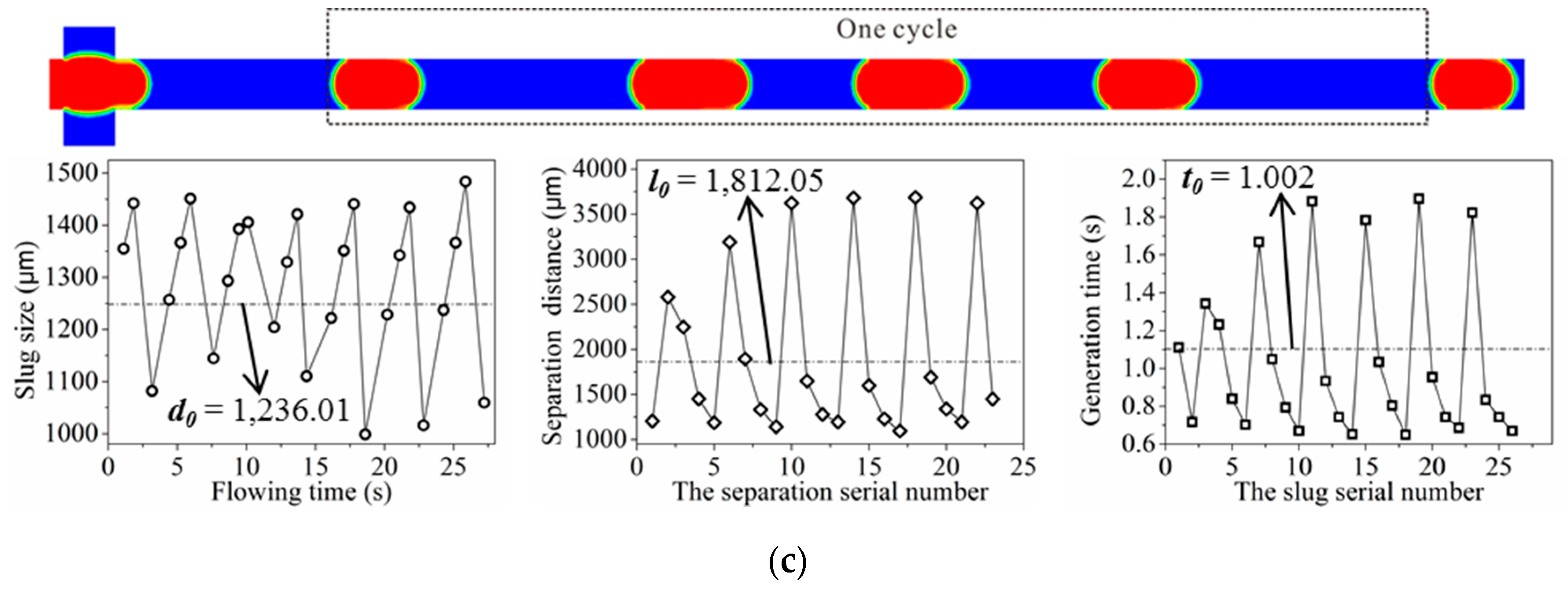
| 0.001 | 0.001 | 1183 | 1236.01 | 4.5 | 1950 | 1812.05 | −7.1 |
| 0.002 | 0.002 | 1066 | 1104.23 | 3.6 | 1518 | 1533.74 | 1.0 |
| 0.003 | 0.003 | 1026 | 986.18 | −3.9 | 1278 | 1288.89 | 0.9 |
| 0.004 | 0.004 | 926 | 934.19 | 0.9 | 1299 | 1243.61 | −4.3 |
© 2019 by the authors. Licensee MDPI, Basel, Switzerland. This article is an open access article distributed under the terms and conditions of the Creative Commons Attribution (CC BY) license (http://creativecommons.org/licenses/by/4.0/).
Share and Cite
Qian, J.-y.; Chen, M.-r.; Wu, Z.; Jin, Z.-j.; Sunden, B. Effects of a Dynamic Injection Flow Rate on Slug Generation in a Cross-Junction Square Microchannel. Processes 2019, 7, 765. https://doi.org/10.3390/pr7100765
Qian J-y, Chen M-r, Wu Z, Jin Z-j, Sunden B. Effects of a Dynamic Injection Flow Rate on Slug Generation in a Cross-Junction Square Microchannel. Processes. 2019; 7(10):765. https://doi.org/10.3390/pr7100765
Chicago/Turabian StyleQian, Jin-yuan, Min-rui Chen, Zan Wu, Zhi-jiang Jin, and Bengt Sunden. 2019. "Effects of a Dynamic Injection Flow Rate on Slug Generation in a Cross-Junction Square Microchannel" Processes 7, no. 10: 765. https://doi.org/10.3390/pr7100765
APA StyleQian, J.-y., Chen, M.-r., Wu, Z., Jin, Z.-j., & Sunden, B. (2019). Effects of a Dynamic Injection Flow Rate on Slug Generation in a Cross-Junction Square Microchannel. Processes, 7(10), 765. https://doi.org/10.3390/pr7100765