1. Introduction
Nowadays, the controlled-source electromagnetic (CSEM) technique is a significant application to detect and discover hydrocarbon-filled reservoirs based on the principles of electromagnetic (EM) propagation. For decades, CSEM application has been widely exercised in onshore geophysical exploration (e.g., [
1,
2]). The efficiency of this application to characterize offshore hydrocarbon reservoirs has also been proven by many oil and gas companies around the world. Li and Key [
3] stated that at early stage, marine CSEM application was employed to study the electrical conductivity of the upper mantle and oceanic crust (e.g., [
4,
5,
6,
7,
8]). Studies related to the commercial application of the marine CSEM technique in offshore hydrocarbon exploration can be found in [
9,
10,
11,
12,
13,
14,
15,
16,
17]. Previously, the seismic sounding survey, which employs acoustic waves, was solely utilized to map geological structures that have different acoustic properties [
18]. This survey was very important to hydrocarbon exploration due to its capability of providing information of the subsurface. According to [
19], seismic data interpretation provides good resolution of the subsurface structures underneath the seabed; however, it has deficiencies. It is said that seismic surveys are unable to distinguish the fluid content inside the reservoirs, whether brine (conductive seawater) or hydrocarbon. Zaid et al. [
18] mentioned that seismic sounding is not compatible to the direct detection of the pore fluid reservoirs. Note that EM and seismic techniques are sensitive to two different properties of subsurface; thus, the marine CSEM technique was developed as a complementary interpretational tool to specifically characterize the target reservoirs.
The marine CSEM technique also is referred to as a seabed logging (SBL) application. This is thoroughly described by [
10]. This application is particularly able to reduce ambiguities in data interpretation in hydrocarbon exploration. Andreis and MacGregor [
16] stated that by studying the reflected EM signal, resistive mediums such as hydrocarbon, gas, and hydrate can be discovered to depths of several kilometers from the seabed. In addition, the resistivity of the subsurface in offshore environments is commonly identified by robust anisotropy because of the sedimentation factor [
20]. Note that for a medium that is horizontally stratified, the subsurface is generally less resistive in the horizontal (parallel) direction than in the vertical (perpendicular) direction [
20]. Offshore hydrocarbon reservoirs are normally embedded in a high conductive medium unlike the common case of onshore hydrocarbon reservoirs [
21]. Hydrocarbon-filled reservoirs are known to have very high electrical resistivity compared to its surroundings, such as of saline water and sedimentary rocks. These structures are very conductive. From [
22], hydrocarbon is known to have electrical resistivity between 30 and 500 Ohm meter, whereas the resistivity values of seawater and sediment are 0.5–2 Ohm meter and 1–2 Ohm meter, respectively. If a target reservoir is brine saturated, it is normally a few orders of magnitude less electrically resistive than a hydrocarbon-filled reservoir. From these characteristics, the resistivity of the subsurface can be resolved via data of electric (E-) and magnetic (H-) fields obtained from the marine CSEM survey. The measurement of amplitude and phase of E- and H- fields can be utilized to determine the geological subsurface. Li and Key [
3] mentioned that the amplitude and phase of an EM field will vary depending on the resistivity of the structures beneath the seabed, the depth of seawater, and the source–receiver offset.
In the marine CSEM technique, data collected can be interpreted in two different groups depending on the domain—either in time-domain or frequency-domain. Analyzing data in time- or frequency-domains would theoretically give the same output/information [
23]. Reyes et al. [
24] mentioned that frequency-domain marine CSEM is normally used for the case of oil prospecting. In the frequency-domain application, an antenna/transmitter of towed EM dipole is generally used to generate a low-frequency EM field, and returned/reflected signals recorded by receivers placed on the seabed are utilized for resistivity distribution analysis. The choice of frequency is very crucial in marine CSEM application. In a standard configuration, marine CSEM surveys use a deep-towed horizontal electric dipole (HED) transmitter to emit a low-frequency EM wave which is usually between 0.1 Hz and 10 Hz to an array of seabed receivers, and normally, the transmitter is towed at 30–50 m above the seabed [
25]. Practically, the low-frequency of EM waves is used in a deep water environment as the signal transmission due to the fact that low-frequency is able to yield farther penetration through seawater columns into sedimentary rocks. Next, for the receiver, there are two types of receiver configurations—inline and broadside. Inline configuration is when the separation distance is parallel to the direction of antenna, whereas broadside is when the source–receiver offset is normal to the antenna’s direction [
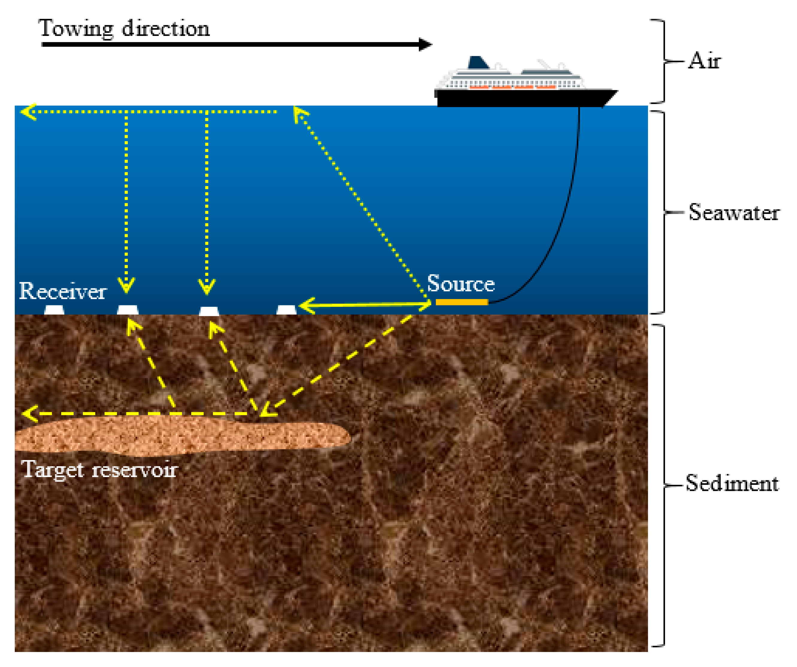
26]. Due to the characteristics of subsurface conductivity, EM signals spread with a higher rate through the seafloor than through the seawater. The EM energy, which is transmitted from the towed-source, spreads in all directions and is quickly attenuated in conductive medium such as sediment. The occurrence of all possible signal contributions is depicted in
Figure 1.
Based on
Figure 1, the straight-line arrow denotes the direct-wave travelling from the source to the seabed receiver without any interaction with the geological subsurface beneath the seabed. Researchers in [
27,
28] mentioned that direct-wave dominates the data collection at short source–receiver separation offsets. Next, the dotted-line arrow represents the reflected and refracted wave from the source upwards to the air–seawater interface and vertically going back through the seawater to the receiver (i.e., air-wave). This wave travels with high rate of velocity (propagates with no attenuation) to the water surface since air is an infinitely electrical resistive medium. Seawater depth can influence the measured EM signal. Air-wave contribution increases as the depth of seawater decreases. Weiss [
29] asserted that this contribution becomes significant in a seawater depth of roughly less than 300 m. Both these signals, direct- and air- waves, do not contain any information about hydrocarbon-filled reservoirs. Last signal contribution is denoted as dashed-line arrow. It is known as the reflected and refracted wave (i.e., guided-wave). This wave diffuses outward from the source through seawater column and then through the high resistive formations with less attenuation. The transmitted wave has to enter the formations at certain angle which is between 0° and 11° in order to set the guided mode [
28]. This reflected and refracted wave strongly dominates the recordings at intermediate source–receiver offsets (~3 to ~8 km). The detection of the guided-wave is the basis of the marine CSEM survey.
In the context of geophysics forward modeling, electrical resistivity has an important role in oil and gas exploration. Numerical modeling is a crucial component that provides information of the electrical resistivity of the subsurface. There are various computational techniques exercised in EM applications such as the Finite Element (FE), the Finite Difference (FD) and the Method of Moment (MOM) [
30], while researchers in [
20] have said that FE, FD and integral equation (IE) methods are among the most famous numerical techniques for modeling EM data. According to [
20], the FE method is more reliable for EM forward modeling in a complex geological structure when compared to FD and IE methods. Based on the literature, FE is a usual numerical technique exercised in CSEM modeling for hydrocarbon exploration. This computational method uses unstructured grids that can be easily conformed to irregular boundaries compared to the FD method. The MOM is less preferred as well in marine CSEM data interpretation since this method produces more complex derivations of governing equations than the FE method. The traditional FD method is easier to implement and maintain than the FE method, but the method is based on structured grids. This means that grid refinement is not possible, and hence it affects the overall computational processes [
31]. Unstructured grids have long been exercised in various fields such as engineering and applied mathematics; however, this feature has only recently been used in the EM geophysical field, as exemplified by the use of FE method code in marine EM surveys (e.g., [
3,
32,
33,
34]). This feature can realistically replicate the complexities of geological structures [
19].
Even though this numerical technique is very powerful, the ad hoc design of meshes in FE is time-consuming. Li and Key [
3] mentioned that the most time-consuming task in their code (FE algorithms) is the solutions of the linear equation systems. The study could take a very lengthy computational time if they used all wavenumbers in the mesh refinement for a full solution. Bakr et al. [
35] also stated that the most time-consuming tasks in FE are evaluating the integrals and solving the linear equations. For typical simulations, a few million elements are involved in the linear equation systems [
31]. According to [
24], the execution of real-field simulations in EM problems needs the use of high-performance computing (HPC). This is because typical actual executions require more than hundred thousand realizations which involve millions of degrees of freedom for each process. The computational and memory requirements to solve such solutions may become a serious challenge. It can be more complicated for higher-dimensional EM forward modeling and inversion. Besides forward modeling, inversion is also a powerful way to recover the electrical conductivity profile beneath the seabed given measurements of EM fields acquired from real-field surveys. Not to mention, nowadays, inverse modeling comes with robust inversion schemes and incorporation of more procedures and measurements. This makes it possible to compute the EM fields at the seabed receivers precisely and provide accurate geometry resolution. However, it is said that inversion algorithms tend to be computationally expensive due to the forward modeling schemes. Indeed, an inversion process needs multiple EM forward solutions [
35]. Furthermore, in terms of application, the marine CSEM technique generates huge amounts of data (captured by seabed EM receivers with a moving HED source); therefore, processing those data has become a challenging task to many geophysicists [
9,
36]. Modeling the marine CSEM data is related to the need of accurate representation of very complex geo-electrical models, and the algorithms used should be powerful and fast enough to be applied to repeated use of hundreds of iterations and multiple source–receiver positions. In addition, understanding the noisy CSEM data to quantify the uncertainties involved in EM modeling also is very crucial. Constable and Srnka [
14] stated that the economic challenges (e.g., related to drilling) increase as the hydrocarbon exploration moves to deeper offshore environments. Thus, any additional data that can be obtained or collected will be advantageous to the exploration if there is a potential to de-risk a given expectation [
19].
In order to seek the most favorable balance between the computational cost involved in the interpretation of EM geophysical data and the accuracy of the modeling, our interest is focused on processing the one-dimensional (1D) frequency-domain marine CSEM data using Gaussian process (GP) algorithms. We propose GP as a methodology for two-dimensional (2D) forward modeling of the marine CSEM technique to provide information on EM profiles when hydrocarbon is present at various depths in isotropic mediums. This forward modeling provides the uncertainty measurement of the estimation in terms of variance. Although the existing CSEM models (the existing numerical modeling techniques) provide robust representation of real-field models, this work has significant contribution for hydrocarbon detection as well. This attempt is very useful and helpful when collected sets of data in CSEM surveys are insufficient for the interpretation of higher-dimensional modeling and inversion. This analysis also could reduce time in the CSEM workflow since forward GP modeling is able to provide uncertainty quantifications without integrating or combining any other numerical quantifiers. On top of that, there is its simplicity, as GP only involves simple equations which means faster computation which only needs basic memory space. Note that this analysis utilizes the simulation datasets generated through a commercial software, namely, Computer Simulation Technology (CST). Information of the CST software can be found in [
37]. The details and literature of GP application are thoroughly elaborated in next section.
2. Statistical Background: Gaussian Process in Computer Experiments
Gaussian Process (GP) is random function which has a property that any finite number of evaluations of the (random) function has a multivariate Gaussian distribution. GP is fully specified by a mean function,
, and a covariance function,
. The Gaussian distribution has mean and covariance values in the forms of vector and matrix evaluations, respectively [
38]. Here,
represents all potential independent variables that influences the outputs/responses. GP is a non-parametric and probabilistic method for fitting functional forms based on domain observations. It differs from most of other black-box identification approaches where it does not approximate the modelled system by fitting the parameters of basis function, but rather searches for relationships among the measured data. This non-parametric regression method does not need a fixed discretization. This technique is able to provide predictive mean values and uncertainty of the estimation measured in terms of variance. This variance reflects the quality of the output/information. It is an important numerical measure when it comes to distinguishing GP from the other computational intelligence methods. According to [
38], GP is suitable for modeling uncertain processes or data which are unreliable, noisy or contain missing values. GP has been used in many different applications. Studies related to application of GP in various fields can be found in [
39,
40,
41,
42,
43,
44,
45]. In general, prior belief of spatial smoothness is specified through a covariance defined by similarity characteristics. Training observations are then considered as the realizations from the updated multivariate Gaussian (i.e., posterior). Thus, the conditional realizations from the posterior are simply the testing output at all untried or unobserved points. The mathematics behind this concept are thoroughly explained in the methodology section.
Computer experiments are well-known and not new in science, technology, and engineering. This medium is getting very popular for solving scientific and engineering problems. Nowadays, scientists prefer to use computer simulators rather than doing case studies or conducting any related physical experiments. It can be implemented in any circumstances including experiments that are impossible to do physically, with shorter time taken than in the real situation. Computer experiments are run by means of a complex code and highly developed theories of physics, mathematics, and engineering fields. Sacks et al. [
46] described that experimenters usually aim to estimate/predict the output at unobserved input points, optimize the function of the output points, and calibrate the computer code to physical data. To this end, [
46] and the subsequent works modelled the output of a computer model,
, based on input
as a sum of regression terms,
, and stochastic component,
.
is defined in Equation (1).
where
is a known function with
, and
is a random process with a zero-mean and a covariance. The most famous choice of the stochastic component,
, is a GP where the distribution of the GP is assumed to be a normal (Gaussian) distribution with a mean and a covariance function. According to [
47], GP is used as the surrogate model for any complex mathematical models which consume a lot of time to solve. GP is flexible in representing the computer output,
, and it is feasible to obtain analytical formulas of the predictive distribution and to design the equations.
From the reported literature, there are a few studies calibrating CST computer output of marine CSEM applications with GP (e.g., [
48,
49]). However, these studies present 1D GP modeling of SBL applications where they only considered univariate independent variables. Besides, the work only focused on predicting the presence of the hydrocarbon layer at a known depth, while we consider various depths of hydrocarbon at observed and unobserved depth levels. This is because the location of hydrocarbon reservoirs can be anywhere and is uncertain in real-field environments. Aris et al. [
50] also described forward GP modeling of SBL applications, but the paper only focused on one transmission frequency and no error was considered in the presented GP modeling. Since CST computer output is assumed to generate very clean data, considering the error in modeling is very important to marine CSEM data processing. Thus, this attempt is novel in two ways; first, it proposes GP methodology to process marine CSEM data calibrated with CST computer output at multiple transmission frequencies at which hydrocarbon is present at all possible depth levels (250–2750 m); second, this is a data-dependent analysis where it utilizes an uncertainty quantification provided by the GP in marine CSEM data processing with error considerations before in-depth analysis. This may enhance the EM data interpretation where the EM profile is estimated with the measurement of variance at various possible depths of the hydrocarbon layer, which helps decision-making for hydrocarbon detection in marine CSEM applications.
3. Methodology
The methodological flow is based on a three-step procedure; (i) synthetic seabed logging (SBL) modeling using Computer Simulation Technology (CST) software, (ii) developing two-dimensional (2D) forward Gaussian Process (GP) models for multiple EM transmission frequencies, and (iii) model validation using the root mean square error (RMSE) and the coefficient of variation (CV).
3.1. Synthetic SBL Modeling Using CST Software
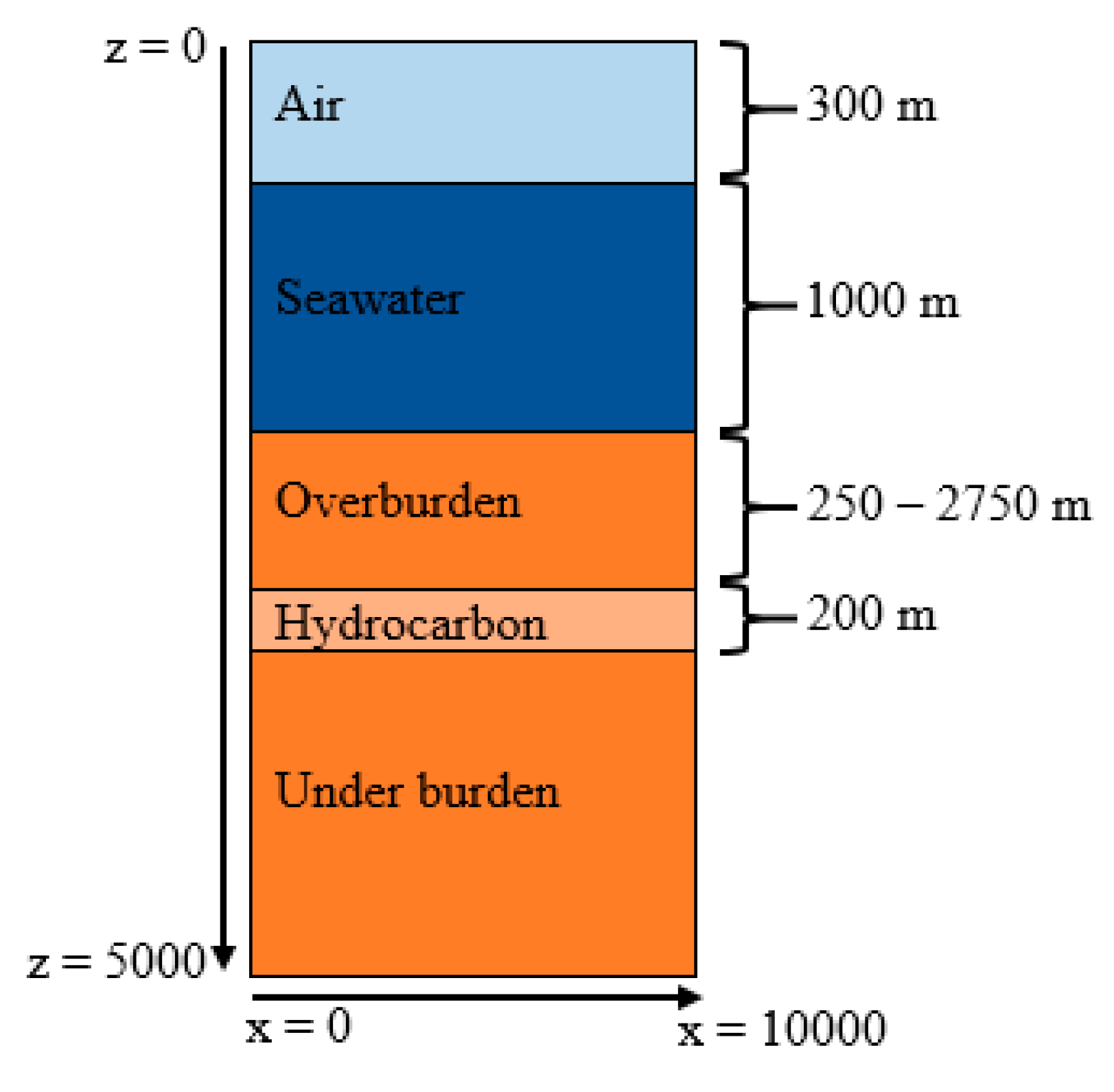
We designed synthetic models of typical marine CSEM application for hydrocarbon exploration which have various depths of hydrocarbon at multiple frequencies by using CST software. The transmissions were tested at frequencies of excitation current of 0.125, 0.25, and 0.5 Hz. Note that in the CST software, Maxwell’s equations are discretized using the Finite Integration Method (FIM). FIM solves the Maxwell’s equations in a finite calculation domain in grid cells to probe the resistivity contrast. For this study, the SBL model is a three-dimensional (3D) canonical structure, which consists of background layers such as air, seawater, and sediment. The model is designed with an air–seawater interface at z = 300 and the seawater thickness is fixed at 1000 m (deep offshore environment). A 200 m-thick horizontal resistive layer (hydrocarbon) is embedded in the sediment layer with various depths from the seabed. The thickness of sediment above the hydrocarbon layer, known as overburden thickness, is varied from 250 m to 2750 m with an increment of 250 m each. The thickness of the overburden layer indicates the depth of hydrocarbon reservoir. Thicker overburden layers mean a deeper location of the hydrocarbon. Both the background and hydrocarbon layers are considered as isotropic.
Figure 2 shows the stratified illustration of the horizontal layers used in this study.
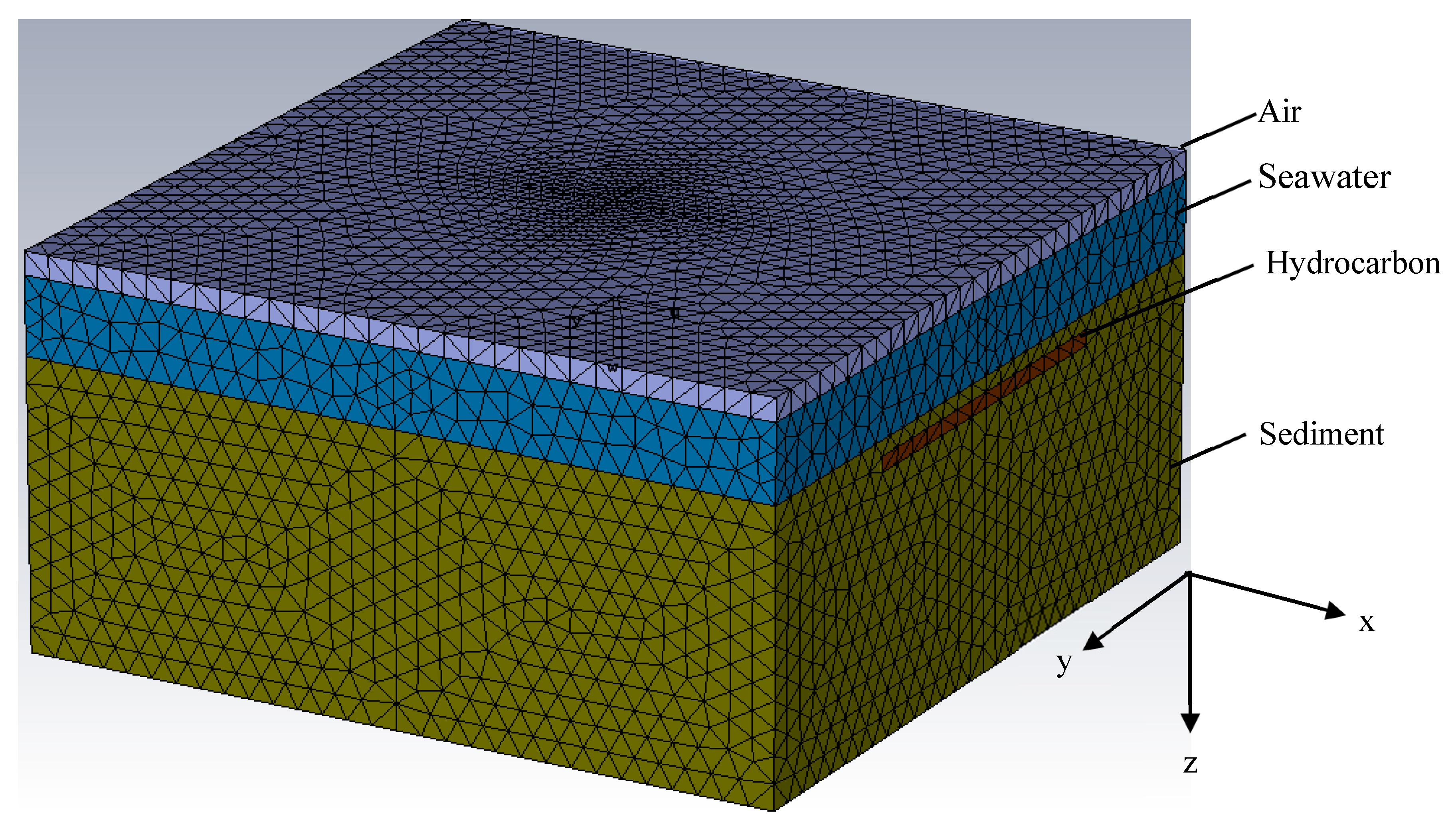
The replication of the 3D structures of the SBL model (length, x: 10,000 m; width; y: 10,000 m; height, z: 5000 m) can be referred to in [
50]. The electrical conductivities of air, seawater, sediment, and hydrocarbon are tabulated in
Table 1. Their properties are taken from [
48].
The EM signal is transmitted by a HED source located with the orientation of
x-direction in the seawater with coordinates (5000, 5000, 1270). This means that the inline transmitter pointing along x-axis is positioned at
,
= 5000, and a height of 30 m above the seabed. The HED source is held stationary at the center of the model. The values of the EM field are measured along an inline profile through the SBL model. In this study, the current strength of the HED source is fixed at 1250 A. The source–receiver separation distances (offsets) are varied along the replication model. An array of 1000 seabed receivers is placed along the seabed at
ranges of 0–10,000 m and y = 5000 m. This means, receivers are positioned along the seabed for every 10 m from 0–10,000 m of x-orientation. As a demonstration,
Figure 3 is the mesh view of the replication of the marine CSEM model in isotropic medium, replicated by the CST software at a hydrocarbon depth of 250 m.
3.2. Developing 2D Forward GP Models at Multiple EM Transmission Frequencies
Let be the CST computer output at different input specifications for every frequency used (0.125, 0.25, and 0.5 Hz), where . The input variable, , can be univariate or multivariate, but in this study, we exercise a bivariate independent variable. Source–receiver separation distance (offset), , and depth of hydrocarbon layer from the seabed, , are considered as input variables where . In this paper, we focus on processing non-normalized CST output, , which is the magnitude of the E-field (amplitude) obtained from static source–receiver combinations where the transmitter is fixed at the center of the SBL model. For every frequency, we have source–receiver separation distances, , and hydrocarbon depths, , which are from 250 to 2750 m with and increment of 250 m each. Thus, in this study, we have different input specifications of CST computer output that are to be processed.
As mentioned earlier, GP is completely defined by a mean function, , and a covariance function, . The GP model on function with a zero-mean function, , and a covariance function, , can be written as
An appropriate correlation function for our GP is selected. The choice of the correlation function is very crucial in computer experiments. It governs the smoothness of the sample path realizations of the GP and is dictated by CST computer output. We choose a popular covariance function which is the squared exponential (SE) function. This covariance function has been widely used in many applications of GP regression and it produces smooth functional estimates. The SE is defined in Equation (3).
where
and
are signal variance and characteristic-lengths scale, respectively. These hyper-parameters need to be properly estimated, and this is usually by optimizing the marginal likelihood. By referring to Bayes’ theorem, we assume that very little prior knowledge about these hyper-parameters are known, and this prior knowledge corresponds to the maximization of marginal log-likelihood. We have three different datasets (three different frequencies). For every dataset, there are 210 data points consisting of offset and hydrocarbon depths as the independent variables corresponding to the magnitude of the E-field as the dependent variable. According to [
39], two-thirds of the total data should be considered as training data points and the remainder will be the testing points. Thus, in this paper, for every three data points, the first two data are set as the training data points. This procedure was implemented for every frequency used.
The GP regression model is assumed to generally have a relationship of the form where the prior joint distribution for the collection of random variables consist of training and testing points are defined as below
The vector
is observed at spatial locations
where
.
denotes the number of training data points generated from CST software, while
is the spatial dimension exercised in this paper. Note that for every hydrocarbon depth,
and
. Next,
is a vector that specifies the predicted values at particular spatial locations
where
.
is the number of all desired observations (i.e., testing data points) where
for each depth. With 140 data per depth, a matrix
is defined using Equation (3) for all pairs involved in the training points. Then,
is determined such that
where
represents a diagonal covariance matrix of the specified additive noise at 5%.
, and
are calculated using Equation (3) where these matrices define the correlation of training–testing data points and testing–testing data points, respectively. Hence,
is predicted at 70 locations of
per depth. Here, matrix
only has input from testing data points and it is derived from prior information. Thus, the posterior conditional GP as in Equation (1), given the information of
,
and
, is written as
Based on the theorem, for every frequency, the Gaussian probability for the random variable with mean, (i.e., the estimated EM profile at observed and unobserved depths of hydrocarbon), and variance, (uncertainty measurement in terms of ± two standard deviations), are defined in Equations (7) and (8), respectively. These equations are the main equations of GP regression.
3.3. Model Validation Using RMSE and CV
To validate our forward GP model, we calculated the root mean square error (RMSE) and coefficient of variation (CV) of the difference between data predicted by GP (estimates) and the data acquired from CST software. RMSE is able to calculate the difference between an estimate and the true value (observation) corresponding to the expected value of root squared loss. CV is calculated as well to evaluate the relative closeness between true values and estimates in percentage. Two random unobserved depths of hydrocarbon which are 900 m and 2200 m were selected for demonstration purposes. The SBL models with these depths of hydrocarbon were simulated separately. The CST computer output was considered as the true values, and the estimate values are the data predicted by GP at the same depths of hydrocarbon. The RMSE and CV between the true values,
, and the estimate values,
, are defined as below
where
is the total number of testing data points, and
is the absolute average of
. The estimates from the 2D forward GP model should match the simulation data acquired from the CST software at all observed and unobserved depths very well up until larger offset distances.
4. Results and Discussion
We implemented this analysis by using GP algorithms in a MATLAB code (built-in function) referred from [
51]. We considered a typical synthetic frequency-domain marine CSEM study with three different transmission frequencies (0.125, 0.25, and 0.5 Hz), a HED source, and an array of receivers. Note that for every depth of hydrocarbon, the simulation was simultaneously run for the three transmission frequencies (three datasets per simulation). Every simulation process took ~15 min to generate the three different datasets. Hence, total computational time for the CST software to compute the EM fields for 11 hydrocarbon depths was approximately 165 min (~2 h and 45 min). In addition, in order to make the data interpretable, a logarithmic scale with base 10 was applied to the magnitude of the E-field for every frequency since it involves very small values.
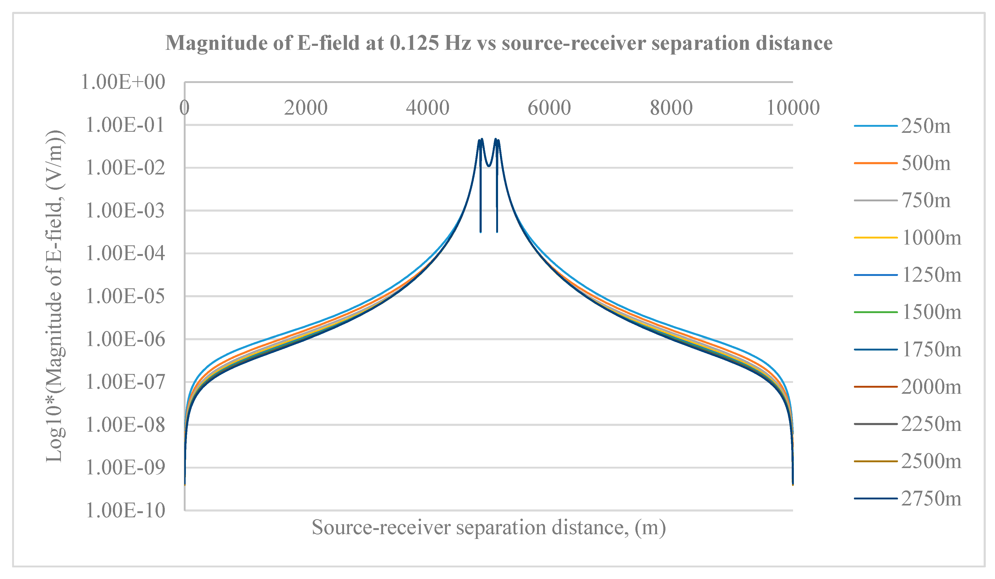
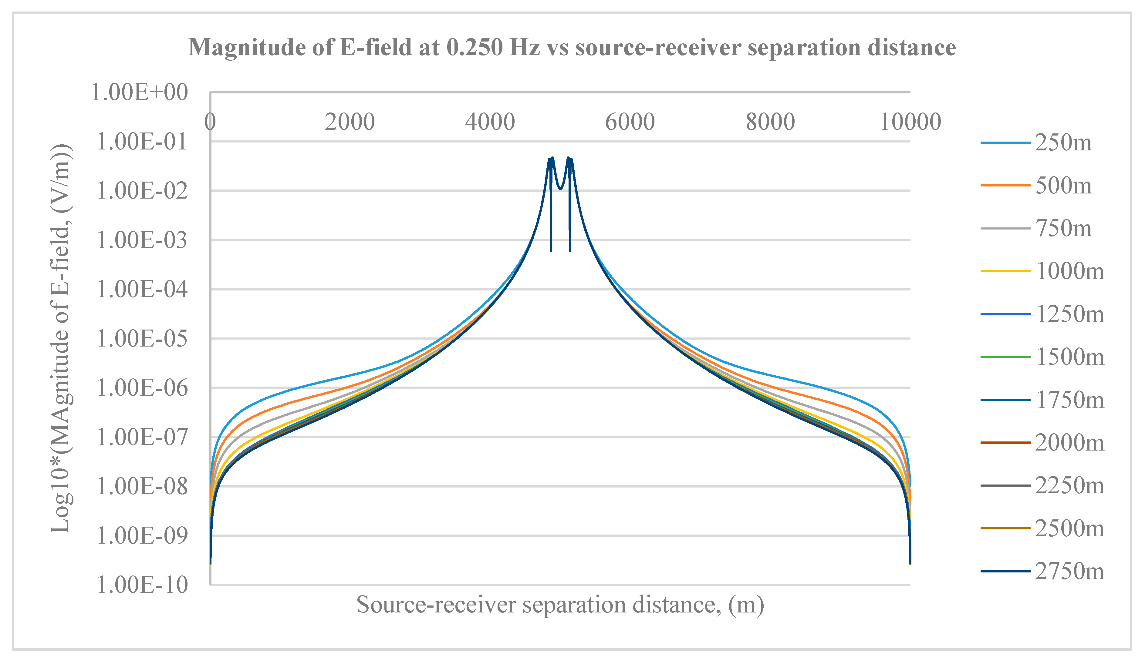
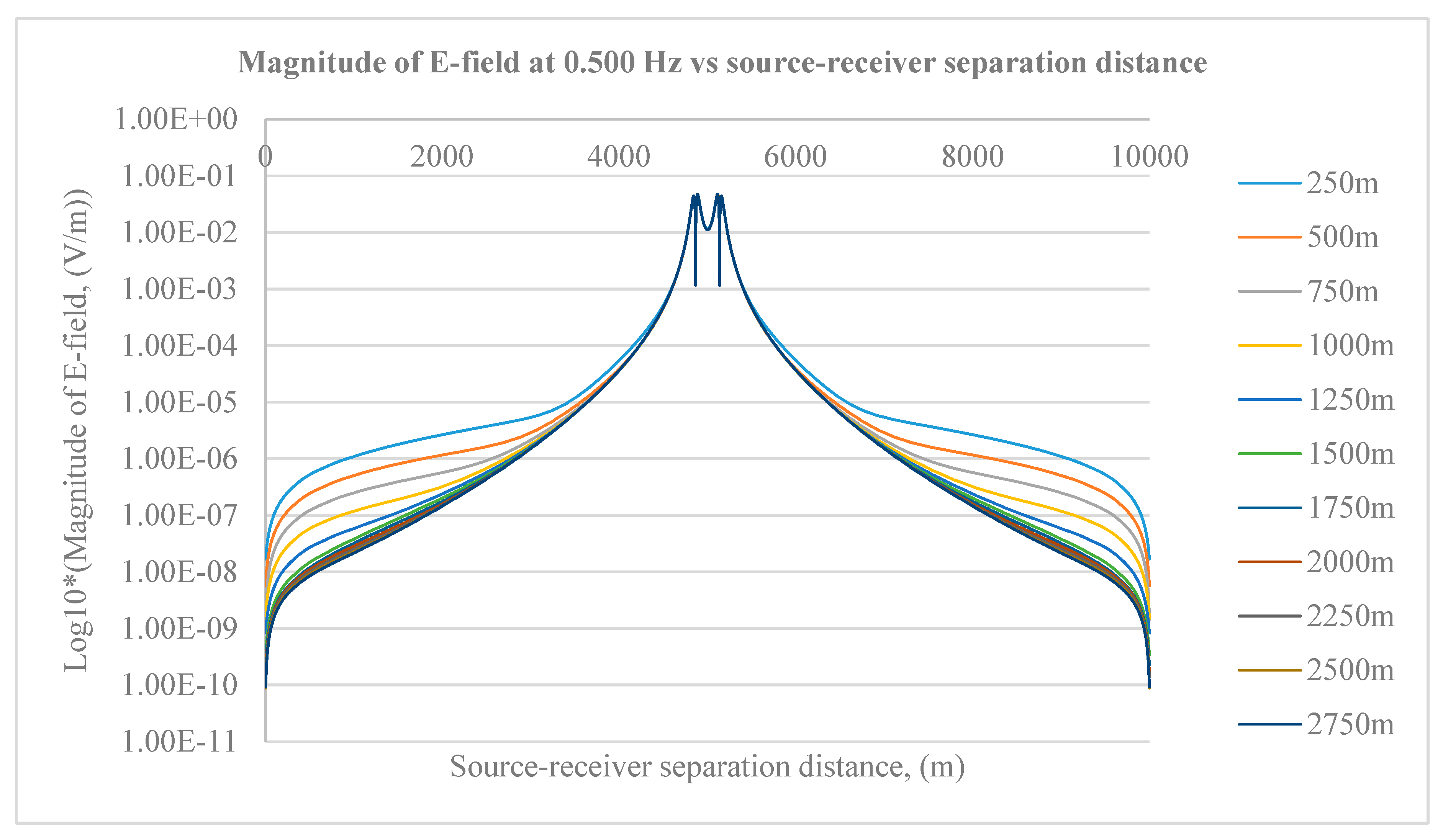
Figure 4,
Figure 5 and
Figure 6 are the CST computer output at all input specifications for every frequency.
From the results, the replicated SBL model is able to reflect the typical synthetic simulation model of EM application. The simulated datasets resulting from the CST software were in a good agreement with the behavior of real-field CSEM data on the effect of the source–receiver separation distance and variations of hydrocarbon depth to the magnitude of the E-field (amplitude). The strength of E-field is inversely proportional to the source–receiver offset and depth of hydrocarbon. If the source–receiver separation is placed further apart and the hydrocarbon layer is located deeper beneath the seabed, the E-field strength significantly decreases. The acquired responses vary in frequency as well. Here, based on figures above, the EM responses are symmetrical. The EM wave was transmitted from the source which was located at the center of the SBL model. The signal travelled equidistant from the source to the boundaries of the model (left and right of the SBL model). Due to this symmetrical setting, only data from 5000 to 10,000 m were considered for processing purposes. Next, from the figures as well, we can see that the magnitudes of the E-field for all hydrocarbon depths are indistinguishable (especially in
Figure 6) at source–receiver offset smaller than ~7400 m. This happens because high transmission frequencies have high attenuation, thus the signal is not able to propagate farther than low-frequency EM wave. Thus, we generalized this analysis by utilizing data for the offset from ~7400 to ~9500 m.
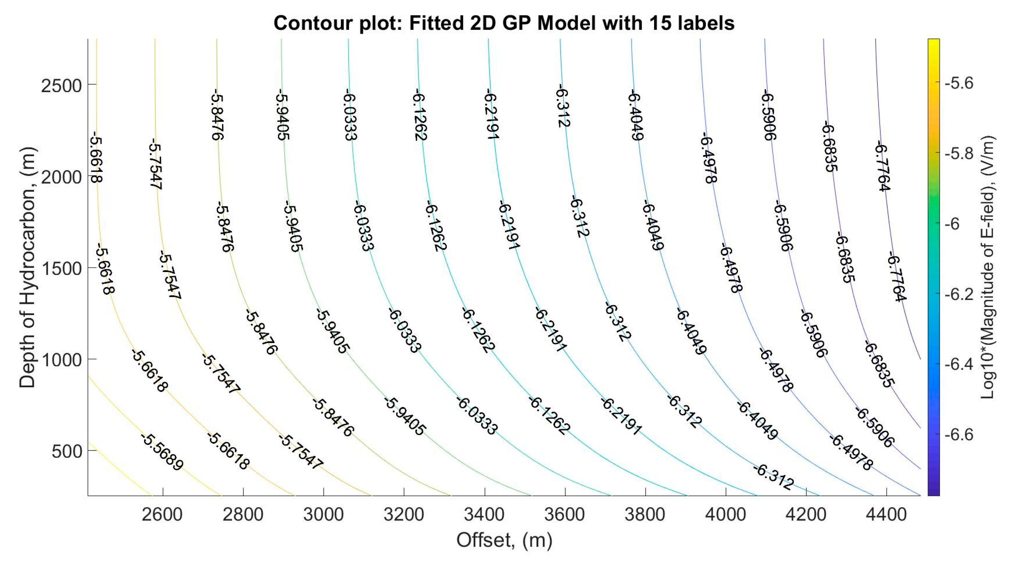
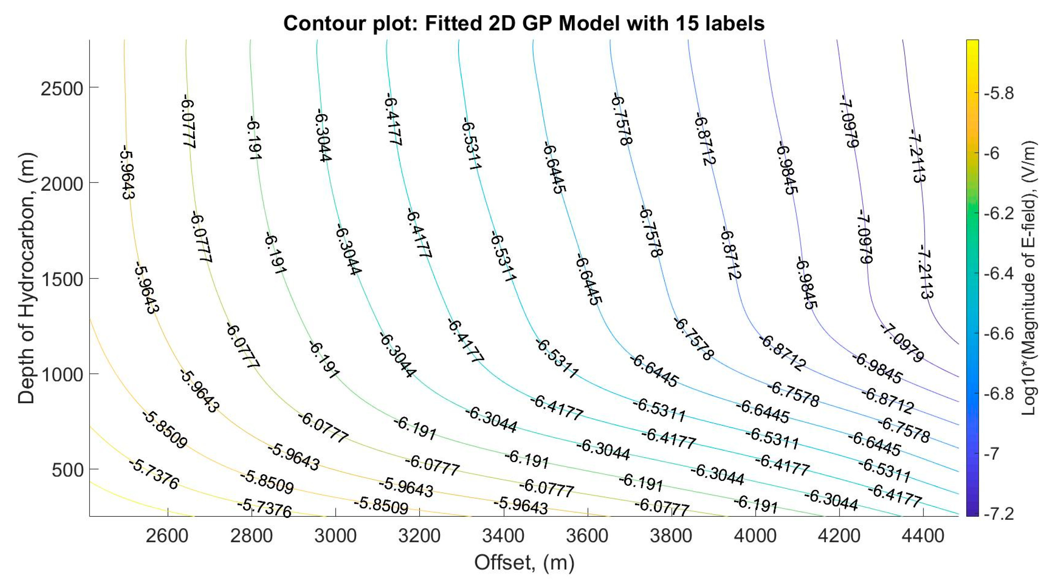
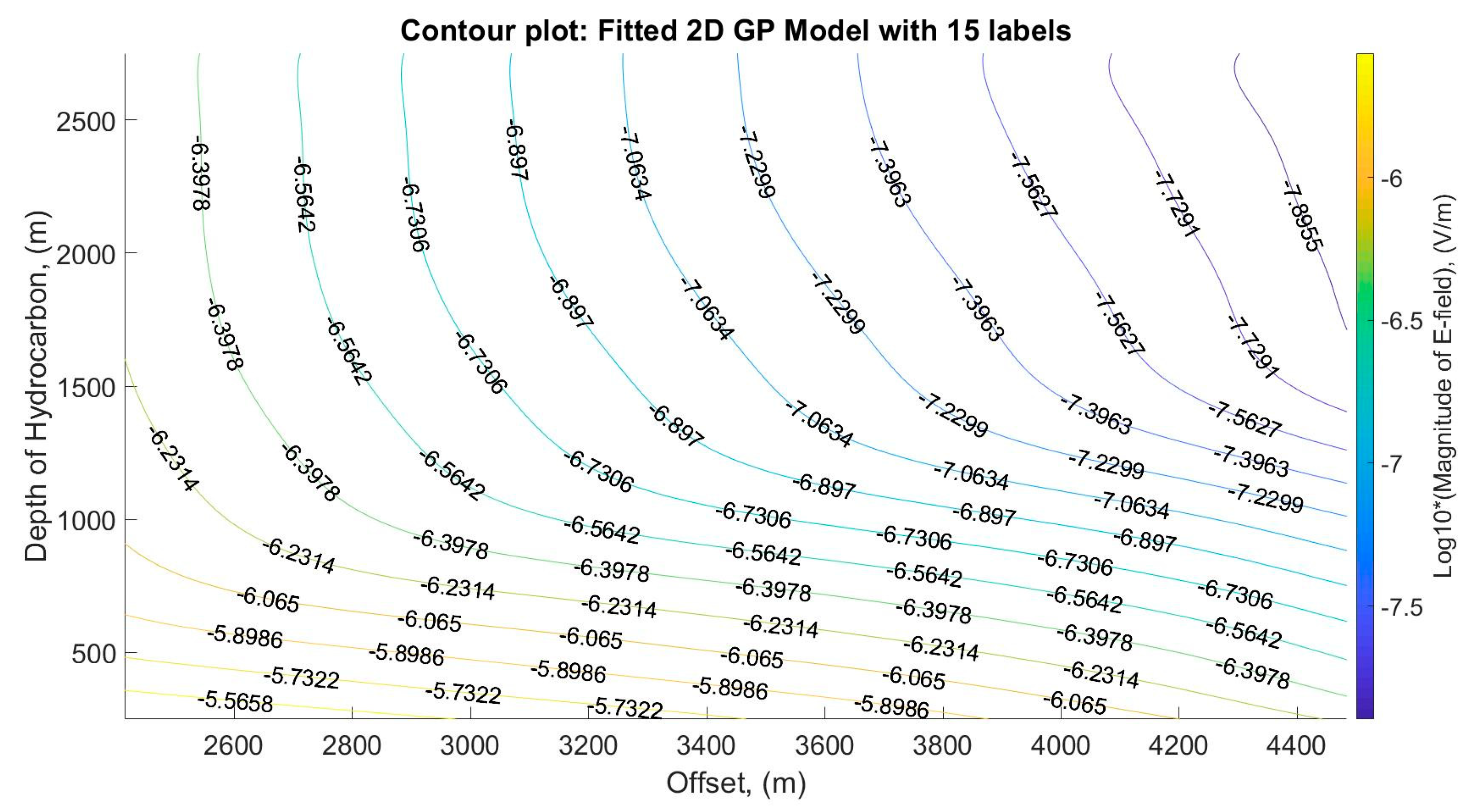
From the CST computer output, we developed a 2D forward GP model for every frequency to provide EM profiles at the observed and unobserved depths of the hydrocarbon. Even though the offset distances considered in this paper are from ~7400 m to ~9500 m, the GP models were set to distances from ~2400 to ~4500 m in order to make it easy to interpret, since the EM signal was transmitted from
(center of the SBL model). The 2D forward GP models for frequencies of 0.125, 0.25, and 0.5 Hz are depicted in
Figure 7,
Figure 8 and
Figure 9, respectively.
From the figures, we can see that the GP models are able to provide the information of EM profiles which are the magnitude of the E-field at all desired depths of hydrocarbon (observed and unobserved). Since variance is quantified in GP estimation, we tabulate the average of the variance of EM profiles for all observed depths of hydrocarbon in
Table 2 to determine how far the data points are spread out from the mean value.
The confidence interval exercised by this paper is 95% of the data which lies within ± two standard deviations of the mean. Small values of variance indicate that the data points tend to be very close to the mean. Based on
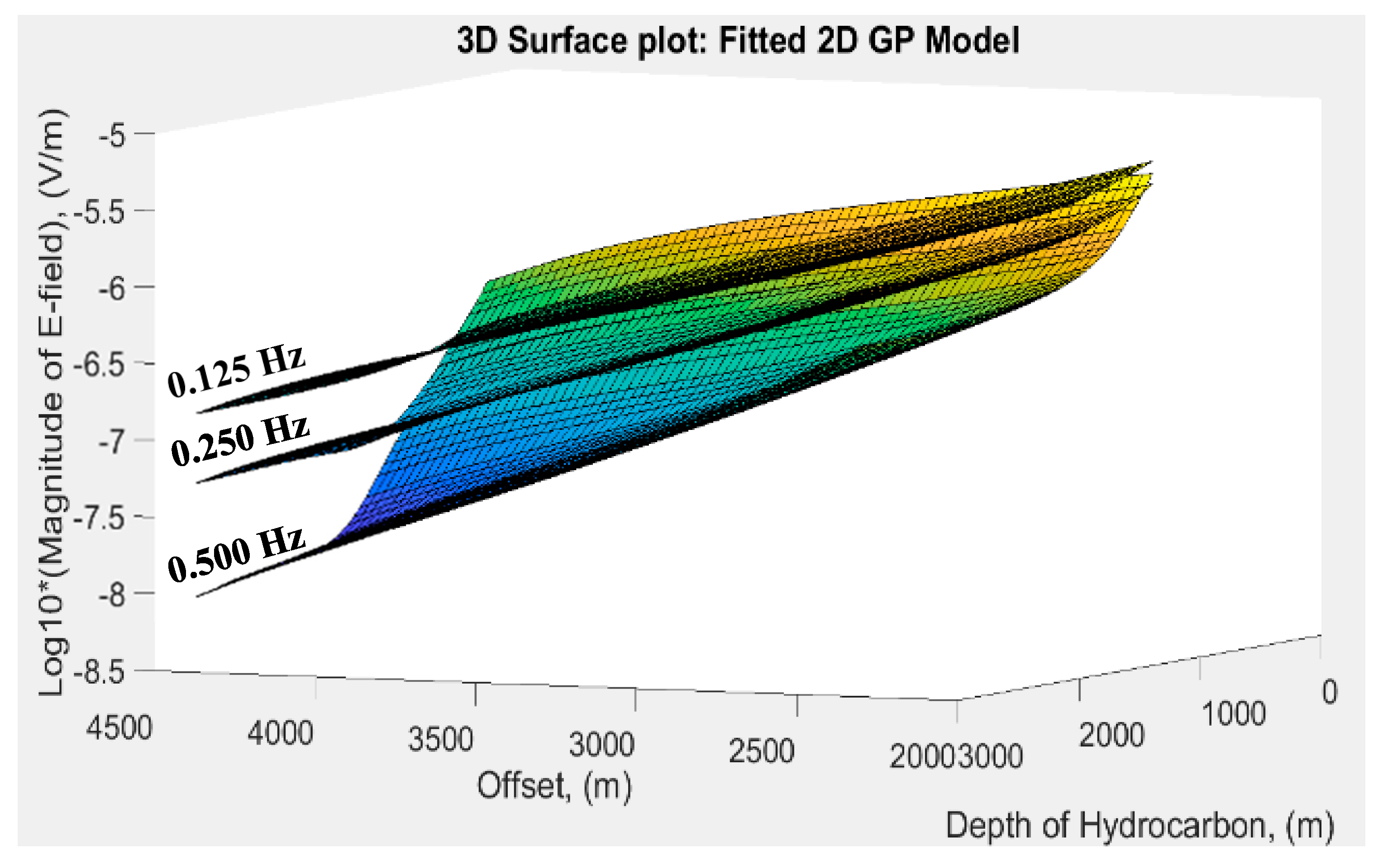
Table 2, all values of the average variances are very small. This implies that the 2D forward GP model is capable of fitting the marine CSEM data very well. Next, for better visualization, we depict a combination of 3D surface plots of the developed 2D forward GP models for every frequency in
Figure 10.
We determined the reliability of these 2D forward GP models in providing the information of EM profiles by calculating the RMSE and the CV between true (data generated through the CST software) and estimate values (data from the forward model) at unobserved/untried depths of hydrocarbon. In this section, random unobserved hydrocarbon depths (900 m and 2200 m) were selected. The EM profiles from these depths were compared with the CST computer output at the same depth levels. The RMSE and CV of the EM profiles at both depths are tabulated in
Table 3.
Based on
Table 3, the RMSE values obtained are very small and all the CVs are generally less than 1%. This means that the modeling results of the 2D forward GP models are in good agreement with the responses acquired from the CST software even at the unobserved/untried depths of hydrocarbon.


