FFANN Optimization by ABC for Controlling a 2nd Order SISO System’s Output with a Desired Settling Time

Abstract

In this study, a control strategy is aimed to ensure the settling time of a 2nd order system’s output value while its input reference value is changed. Here, Feed Forward Artificial Neural Network (FFANN) nonlinear structure has been chosen as a control algorithm. In order to implement the intended control strategy, FFANN’s normalization coefficient (K), learning coefficients (ŋ), momentum coefficients (μ) and the sampling time (Ts) were optimized by Artificial Bee Colony (ABC) but FFANN’s values of weights were chosen arbitrary on start time of control system. After optimization phase, the FFANN behaves as an adaptive optimal discrete time non-linear controller that forces the system output to take the same value with the input reference for a desired settling time (ts). The success of the optimization algorithm was proved with close loop feedback control simulations on Matlab’s Simulink platform based on 2nd order transfer functions. Also, the success was proved with a 2nd order physical system (buck converter) that was structured with power electronics elements on Simulink platform. Finally, the success of the control process was discussed by observing results.

1. Introduction

Nowadays, optimization of controllers’ parameters is preferred for obtaining a better cost-effective control strategies. In the last two decades, researchers have developed different types of optimization algorithms that may be used by scientists in control area. Bee [1], Firefly [2], Bat [3], Virus [4], Genetic [5], Cuckoo [6], Particle Swarm [7], Gravitation [8] and Biogeography [9] may be given for example.

The mathematical algorithms called controller are used for shaping the output variable of a physical system according to a desired behavior [10]. These mathematical algorithms are run using discrete or continuous time hardware [11]. Controller’s parameters are calculated with analysis of rules sequences developed for related control algorithms [12].

Owing to the fact that the Artificial Intelligence algorithms are versatile, with the same type of structure they may be used for solving more than one type of problems such as control, prediction, estimation and modelling [13]. Using the same type of Artificial Neural Network structure, different researches have solved different type of problems. For example, Erkaymaz et al. estimate the thermal performance of a solar air collectors and predicted the modules of rupture values of oriented strand boards [14], Beg et al. proposed a discrete wavelet transform approach to classify power system transient analysis [15], Zounemat-Kermani et al. developed models to predict one day ahead stream flow of the Marion Junction station in Cahaba watershed [16] and Ardestani et al. suggested to predict contact force at the medial knee joint [17].

The most popular type of Artificial Neural Networks (ANN) are illustrated like Feed Forward, Kohonen, Radial Basis, Dynamic Neural, Multilayer Perceptron, Neural-Fuzzy, Cascading Neural and Stochastic Neural [13,14,15,16,17].

There are several studies in the literature that combine heuristic-based optimization algorithms with ANN based algorithms. In some studies, the optimized ANN algorithm is asked to model a system [18,19]. In another type of work, the optimized ANN is expected to work as a predictor [20,21]. There are also several studies in the estimation and control field performed by the ANN algorithm which has been optimized by heuristic algorithms [22,23,24]. The common point of the study types mentioned above is the optimization of the weights of the ANN algorithm. In these works, external parameters of the ANN are not put into optimization. They are fixed in arbitrary way.

In this study, the external parameters that are Kout, η, µ and Ts of the Feed Forward Artificial Neural Network (FFANN) were optimized using the Artificial Bee Colony (ABC) algorithm. The weights, which are the internal parameters of the FFANN algorithm, were randomly assigned and continuously recalculated using the Back-Propagation method in the control process. Thus, the FFANN algorithm is adapted to adaptive and optimal operation.

There are various swarm-based optimization methods in the literature. Such methods present extremely superiority in obtaining the global optimum and in handling discontinuous and non-convex objectives. However, many of these methods are not effective in managing optimization problems of integer and discrete nature. Such optimization problems can be solved by approximating the discrete and integer variables by continuous variables. Thus, the problem becomes an ordinary nonlinear programming one with continuous control parameters and the continuous values are reduced to the closest possible discrete or integer variable values. In practice, this method generally causes to the solutions that may be far from the globally optimal solution. ABC algorithm is a search method, which is inspired by the foraging behavior of honey bee swarming, and target discrete optimization problems [25].

2. The Feed Forward Artificial Neural Network (FFANN) Model

Block diagram belongs to FFANN that was used in this study is given in Figure 1. Here, the FFANN controller has 3 layers called input, hidden and output. Each layer quantity is 1.

Variables in Figure 1 are described as,

$S_1^h,S_2^h,\dots ,S_5^h$ : Addition centers of hidden (h) layer

$w_{11}^h,w_{12}^h,\dots ,w_{15}^h$: Weights between FFANN input and hidden layer addition centers

$w_{21}^h,w_{22}^h,\dots ,w_{25}^h$: Weights, between bias input and hidden layer addition centers, belong to input layer

$R\left(k\right)$: FFANN input

$U\left(k\right)$: FFANN output

$S_1^y$: Addition center of FFANN output layer

$w_{11}^y,w_{21}^y,\dots ,w_{51}^y$: Weights between output of hidden layer and output layer addition center of FFANN

$w_{61}^y$: Weight between bias input of output layer and addition center of output layer

$f\left(x\right)$: Activation function

In the literature, there is not any rule for numbering of hidden layers and for numbering of hidden layer’s neurons [26]. On one hand, if number of hidden layers or neurons is chosen more than needed, the trading volume would be increased unnecessarily while optimizing the weights; on the other hand, if they were chosen less than needed, probability of reaching the level of acceptable minimum error would be decreased.

In this study, the control structure shown in Figure 2 was constructed. FFANN hidden layers and neurons count were determined by experimental observation. To this end, FFANN was optimized by ABC by selecting the hidden layer and the number of neurons high. Then, the optimization process was repeated by selecting the hidden layer and the number of neurons low. Fault-based cost function value was observed by running the control system after optimization process, Equation (11). The results of the experiment showed that the FFANN-based control process involved a high number of hidden layers and neurons, and the cost value of the FFANN-based control process with a low amount of hidden layer and neuron was similar, Figure 8. Considering the cost function values of the experimental processes, the numbers of hidden layers were chosen as 1 and the numbers of neurons belonging to the hidden layer were chosen as 5, Figure 1.

Another important variable is the activation function. The function type has also effects on weight optimization [27]. The FFANN controller in the closed loop negative feedback control system generates the control signal, u(k), based on error signal, e(k), Figure 2. The error during the control process may be greater, lower or equal to zero. Therefore, the activation function with limit values [−1, +1] of tangent sigmoid is chosen in the FFANN structure, Equation (1).

$$f\left(x\right)=\frac{e^x-e^{-x}}{e^x+e^{-x}}$$

(1)

3. The Control System

Block diagram of close loop negative feedback control system based on FFANN controller is shown on Figure 2. Here, the controller is a discrete time algorithm but the system that is under control has continuous time structure.

For this study, a Digital to Analog Converter (DAC) was chosen, with a 1st order holder transfer function, as seen Equation (2).

$$\frac{1-e^{sT}}{s}$$

(2)

Since operation range of a FFANN is between [−1, +1] [28], input signals have to be involved into FFANN algorithm only after multiply by normalization coefficient (Kin). FFANN’s output signal is turned back using de-normalization coefficient (Kout) as shown in Figure 2.

FFANN algorithm is a two-step mathematical algorithm. In the first step, optimization of FFANN weights is done. In literature, this step is named as “learning process”. In this study, “Steepest Descent” method has been used for weight optimization. This optimization method is simple structured and fast [28]. Renewal of weights based on this method is given in Equation (3) and Equations (3) and (4).

$$E\left(k\right)=\frac{1}{2}{\left(R\left(k\right)-Y\left(k\right)\right)}^2$$

(3)

$$w\left(k+1\right)=w\left(k\right)-\eta \frac{\partial E\left(k\right)}{\partial w}+\mu \left[w\left(k\right)-w\left(k-1\right)\right]$$

(4)

Here, η is learning coefficient and is chosen randomly in the range of (0, 1]. Another coefficient, µ, is momentum coefficient. Momentum coefficient does not only ensure to pass the local gradients but also helps to decrease the proportion of the error. The network may have an oscillation without momentum. Momentum coefficient usage prevents the network from oscillation during learning process, [28]. In literature momentum coefficient is chosen randomly between (0, 1].

At the second step of FFANN, output calculation is realized for sampling moment (Ts × k, k = 0, 1, 2…) as shown in Equations (5)–(7).

$$S_j^h={\displaystyle \sum _{i=1}^5\left(R\left(k\right)w_{ji}^h\right)+}{w}_{2j}^h,\mathrm{j}=1,2,\dots ,5$$

(5)

$$S_1^y={\displaystyle \sum _{i=1}^5\left(f\left(S_i^h\right)w_{i1}^y\right)+}{w}_{61}^y$$

(6)

$$U=f\left(S_1^y\right)$$

(7)

4. Artificial Bee Colony (ABC) Algorithm

A bee transforms itself into a scout bee in order to find new sources when the food source is exhausted. Food source represents cost function in ABC algorithm. Therefore, the lowest cost function value represents the richest food source [29].

Food sources are created randomly in the first step of the algorithm. The bees that go directly to source of food are known as worker bees. Onlooker bees live in colony that they are directed to food sources based on the signs of worker bees. Onlooker bees go to food sources. They chose and store food like worker bees and return to the colony, Figure 3. Worker bees who consume food resources within a certain number of trials turn into scout bees to search for new food sources. When scout bees reach a random food source, process of food storage restart. These steps, continue until end criterion is satisfied [29].

“limits” and “popsize” is two fundamental variables in ABC algorithm. “popsize” is number of individuals in algorithm. The “limit” is number of trials for worker bees to leave food source. If it is not possible to develop as much as the limit value for a solution that represents a resource it is abandoned [29].

The bee that abandoned food source becomes a scout bee. In the ABC algorithm, the number of onlooker bees, number of worker bees and number of food sources equal to each other. Number of food sources is half of the population [29].

First, food sources are created randomly for starting to run ABC algorithm, as seen in Equation (8).

$$x_{i,j}=x_j^{\min }+rand\left(0,1\right)\left(x_j^{\max }-x_j^{\min }\right)$$

(8)

The new solution that is found by worker bees is compared with the old one. If the new solution is better, it keeps this solution and deletes the old solution from memory. If the new solution is not better than before, the previously defined abandonment counter is incremented. Searching food source by worker bees is shown in Equation (9).

$$v_{i,j}=x_{i,j}+{\phi }_{i,j}\left(x_{i,j}-x_{k,j}\right)$$

(9)

After the worker bees have completed their food scan, onlooker bees go to random analysis so that they can select of food sources for bees, Equation (10).

$${\rho }_i=\frac{fi{t}_i}{{\displaystyle \sum _{i=1}^{NS}fi{t}_i}}$$

(10)

The $\rho$ value is obtained for each solution. Worker bees compare ${\rho }_{ref}$ that are randomly selected and used as threshold value with ${\rho }_i$. If the probability of selecting ${\rho }_i$ is larger than ${\rho }_{ref}$ onlooker bee is moved toward this source of food and starts searching for a new solution by rerunning Equation (8).

The variables in Equations (8)–(10) are

$NS$: Number of food sources

D: Number of parameters that are optimized

$x^{\max },x^{\min }$: Limit values of parameters that will be optimized

$v_i$: New food location in relation to $x_i$

$x_k$: Randomly food location that is different from $x_i$

${\phi }_{i,j}$: Random value between −1 to 1

$fi{t}_i$: Normalized cost function

k: Solution in the neighborhood of i

All worker and onlooker bees check the abandonment counter for each solution after completing of food searching. If counter value reaches to limit value, the worker bee turns into a scout bee and run Equation (8). The process steps continue until the maximum number of cycles or the lowest value of the cost function value is reached.

5. Parameter Optimization by ABC

The FFANN weights in the closed-loop control system projected in Figure 2 are optimized during the control process by running the Back-Propagation algorithm. Before starting the control process, the parameters of Kout, η, µ and Ts should be optimized. They are optimized by the heuristic ABC algorithm. In the optimization process, the control system given in Figure 2 is used, too. During the process, the FFANN weights are randomly assigned for each optimization simulation, as in the beginning of the control process, Figure 2.

The implementation of the block diagram of the optimization process described in flow diagram below is given in detail in “Appendix A”. As seen in the block diagram, the FFANN parameters are randomly assigned before the 1st run is performed. Then, the closed loop control system runs up to the simulation time period, Figure 5.

The input reference voltage applied to the control system has square waveform, Figure 4. The corners of the square wave are rounded off using the 1st order transfer function. The square wave is defined as the high and low time interval ts of the reference input voltage. In this way, the ABC algorithm optimizes FFANN parameters for the time interval of the closed-loop control system for the time period specified by ts.

Errors calculated by running the cost function during the simulation are collected. The total error obtained after the simulation is transferred to the ABC algorithm. The ABC algorithm calculates the new Kout, η, µ and Ts parameters by processing the total error within the framework of its mathematical algorithm. Next, the new parameters are replaced with the old ones for use in the next simulation. Prior to running the control system with the new parameters, the weights of FFANN are randomly assigned.

The potential solutions performed by the ABC algorithm, as in other heuristic algorithms, tries to find the closest value to the global solution by moving around instead of finding the most optimal solution available in the problem space [28]. It was also tried to be eliminated by the simulation technique in order to keep the algorithm around a certain local minimum. Therefore, FFANN weights are assigned randomly before running the required simulation for each new cost function account.

Discrete time cost function of Integral Squar Error (ISE) was benefited to determining cost belong to process of control [28]. Mathematical equation belong to discrete ISE is given in Equation (11).

$$ISE\left(e\right)={\displaystyle \sum _{k=0}^{t_{sim}/T_s}{e}_k^2}$$

(11)

ABC optimization process “run ABC” belongs to flow chart in Figure 5 is summarized as:

• Initialize the population of solutions.
• Evaluate the population.
• cycle = 1
• repeat
• Produce new solution (food-source positions) $v_{i,j}$ in the neighborhood of $x_{i,j}$ for the employed bees using Equation (9).
• Apply the greedy selection process between $x_i$ and $v_i$.
• Calculate the probability values of ${\rho }_i$ for the solutions $x_i$ by means of their fitness values, Equation (10).
• Produce the new solutions (new positions) $v_i$ for the onlookers from the solutions $x_i$ selected depending on ${\rho }_i$ and evaluate them.
• Apply the greedy selection process for the onlookers between $x_i$ and $v_i$.
• Determine the abandoned solution (source), if exists, and replace it with a new randomly produced solution $x_i$ for the scout, Equation (8).
• Memorize the best food source position (solution) achieved so far.
• cycle = cycle + 1.
• until cycle = Maximum Cycle Number.

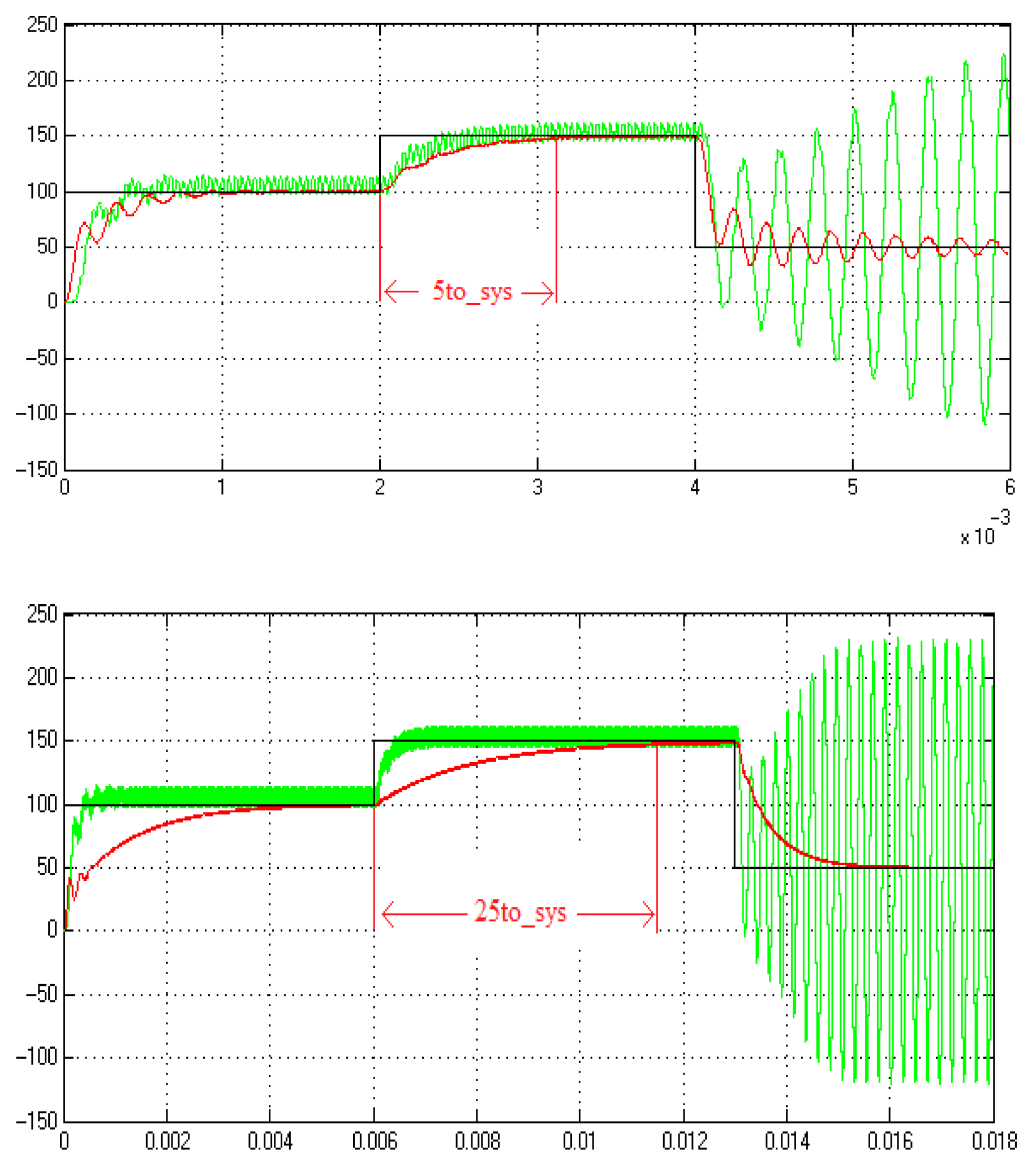
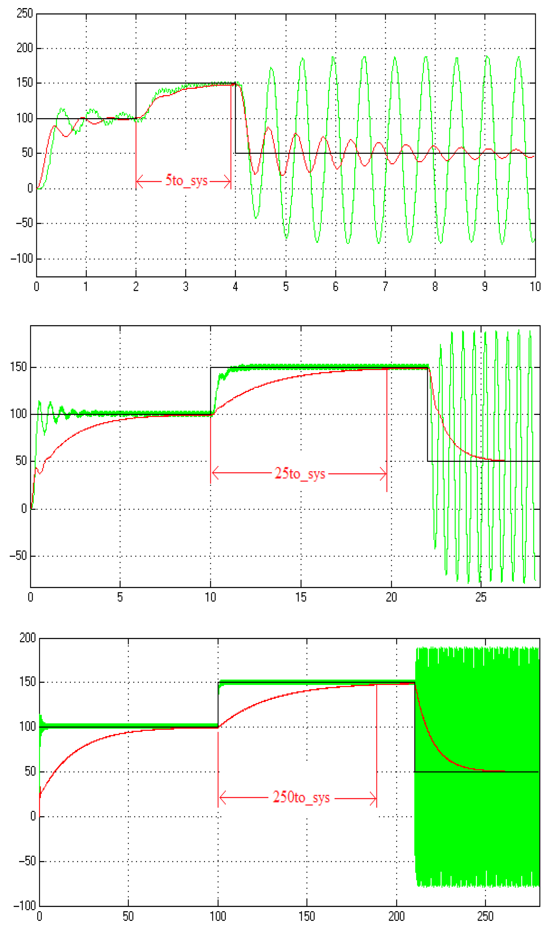
6. Control Simulations with Transfer Functions

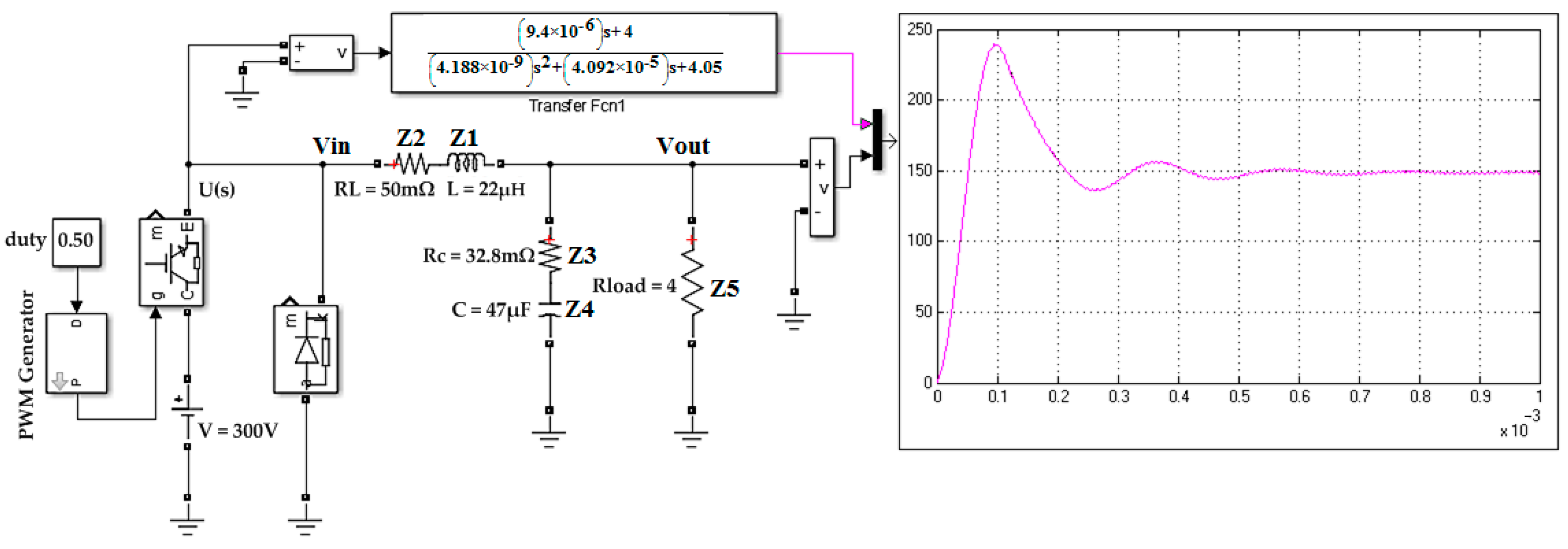
The 2nd order transfer function belongs to a buck converter, Figure 6, can be derived using circuit theory.

$$V_{out}(s)=V_{in}(s)\frac{(Z3+Z4)//Z5}{(Z1+Z2)+(Z3+Z4)//Z5}$$

(12)

$$\frac{V_{out}(s)}{V_{in}(s)}=T\left(s\right)=\frac{\frac{(Z3+Z4)Z5}{Z3+Z4+Z5}}{(Z1+Z2)+\frac{(Z3+Z4)Z5}{Z3+Z4+Z5}}$$

(13)

where,

• $Z1=j\omega L=sL$: Impedance of coil
• $Z2=R_L$: Serial equivalent resistance of coil
• $Z3=R_c$: Serial equivalent resistance of capacitor
• $Z4=\frac{1}{j\omega C}=\frac{1}{sC}$: Impedance of capacitor
• $Z5=R_{load}$: Load resistance
• denotes.

If the impedances are changed with S-domain parameters, the new transfer function takes shape as shown below:

$$T\left(s\right)=\frac{sC{R}_C{R}_{LOAD}+R_{LOAD}}{s^2\left(CL{R}_C+CL{R}_{LOAD}\right)+s\left(L+C{R}_L{R}_C+C{R}_L{R}_{LOAD}+C{R}_C{R}_{LOAD}\right)+\left(R_L+R_{LOAD}\right)}$$

(14)

If variables of T(s) are replaced with parameter values that are used for T₂(s),

Table 1. Buck converters’ parameters.

Equation	L (µH)	Rl (mohm)	C (µF)	Rc (mohm)	Rload (ohm)
6.4	1	50	1	6.6	25
6.5	22	50	47	32.8	4
6.6	2200	50	3300	327.9	50

, it will be seen that T(s) output signal values are the same with the buck converter output voltage for the same input control signal, U(s), Figure 6.

In this study, transfer functions with 3 different time constant (τ) were chosen for control application experience, Equations (15)–(18).

$$\begin{array}{l}{T}_1(s)=\frac{\left(1.25\times {10}^{-6}\right)s+25}{\left(2.505\times {10}^{-11}\right)s^2+\left(3.502\times {10}^{-6}\right)s+25.05},\\ roots=\left(-0.6991\mp 9.9755\mathrm{j}\right)\times {10}^5,\tau =14.3\times {10}^{-6}\end{array}\}$$

(15)

$$\begin{array}{l}{T}_2(s)=\frac{\left(9.4\times {10}^{-6}\right)s+4}{\left(4.188\times {10}^{-9}\right)s^2+\left(4.092\times {10}^{-5}\right)s+4.05},\\ roots=\left(-0.4885\mp 3.0712\mathrm{j}\right)\times {10}^4,\tau =204.69\times {10}^{-6}\end{array}\}$$

(16)

$$\begin{array}{l}{T}_3(s)=\frac{\left(8.25\times {10}^{-3}\right)s+50}{0.3634s^2+2.217s+50.05},\\ roots=\left(-3.0500\mp 11.3331\mathrm{j}\right),\tau =327.9\times {10}^{-3}\end{array}\}$$

(17)

Table 1, indicates the component values of buck converter circuits belong to transfer functions of T₁(s), T₂(s) and T₃(s).

Chosen 3 systems have been adjusted as to have large difference between τ of each other’s. The behaviors of systems’ output signals based on unit step input function have been represented on Figure 7.

On Figure 7, it’s seen that when a unit input signal is applied to transfer functions, overshoot of output signals is different from each other’s. Here the settling times are different for about 1000 times with each other’s. Control success for these 3 transfer functions, whose settling time values are very different from each other will show that the FFANN control logic based on the proposed ABC heuristic optimization method is applicable to all 2nd order systems.

Timing of ABC algorithm was defined by transfer functions’ time constants,

Table 2. Initialization ABC’s timing parameters.

T. Functions	Simulation Time	Iteration
T1(s)	ts1 × 5	100
T2(s)	ts2 × 5	100
T3(s)	ts3 × 5	100

.

On Figure 8, ISE(e) decreasing is shown for optimization process with ABC for $T_1(s)$ and for settling time $t{s}_1=5\tau$. On Figure 8, it is seen that after 14th iteration the cost function becomes stable and so it’s found out the optimum parameters’ values according to ABC algorithm.

In this study, ts values have been chosen according to time constant of systems,

Table 3. Feed Forward Artificial Neural Network (FFANN) parameter optimization for T₁(s).

Setling Time	n1, n2	µ1, µ2	Kout	Tsample
5τ	0.0018	0.038	4725	286 ns
25τ	0.0022	0.052	4455	1.36 µs
250τ	0.0012	0.027	4275	12.584 µs
10,000τ	0.0033	0.041	3825	572.16 µs

,

Table 4. FFANN parameter optimization for T₂(s).

Setling Time	n1, n2	µ1, µ2	Kout	Tsample
5τ	0.0011	0.029	4630	4.094 µs
25τ	0.0034	0.024	4316	20.47 µs
250τ	0.0016	0.028	3804	198.7 µs
10,000τ	0.0027	0.033	3710	8.26 ms

and

Table 5. FFANN parameter optimization for T₃(s).

Setling Time	n1, n2	µ1, µ2	Kout	Tsample
5τ	0.0021	0.027	4722	6.6 ms
25τ	0.0024	0.021	4386	32.8 ms
250τ	0.0019	0.034	3854	319 ms
10,000τ	0.0031	0.028	3635	13.11 s

. FFANN’s optimized parameter values by ABC belong to three different transfer functions for 5 different settling times as shown in Table 3, Table 4 and Table 5. Parameter values of Kin for normalization had been fixed to 1/450 before optimization process was started. Value 450 is 3 times bigger than maximum input reference value (R(k)) that will be applied to the input of the control system, Figure 2.

Control simulations of Figure 2 for T₁(s), T₂(s) and T₃(s) are shown on Figure 9, Figure 10 and Figure 11. It’s seen that success of control with optimal FFANN’s parameters (red output line) is much better than those of with classical chosen FFANN’s parameters (green output line). Here, n₁ = n₂ = 0.1, µ₁ = µ₂ = 0.1, Kout = 1/Kin = 450 and Tsample = τ/10 were chosen as un-optimal FFANN’s parameters.

The control success of the FFANN based controller assigned with the traditional method depends on the roots of the system it is going to control and therefore the time constant exists, see Figure 9, Figure 10 and Figure 11. The response rate of the controller for some systems is sufficient and the system output is close to the input reference value as soon as possible. However, the settlement time of this convergence varies depending on whether the reference step takes up or downward value, Figure 9. The FANN based controller, whose parameters are assigned in the traditional way, can transform the controlled system output into a highly oscillating or marginal stable structure, as shown in Figure 10 and Figure 11. However, the FFANN parameters will be optimized by ABC and the control processes to be performed will be determined in a stable manner. By running the optimization algorithm over the linking strategies of the control process, such as settlement time, more functional output signals based on simpler structured input reference value can be obtained, see Figure 9, Figure 10 and Figure 11.

7. Control Simulations with Power Electronics Components

In Figure 12, a buck converter circuit based on feedback control system is shown. Here, the buck converter transfer function is 2nd order as shown in Section 6, Figure 6. So, Figure 12 shows FFANN based controller for a feedback control system with 2nd order model constructed by hardware on simulation platform.

Control system given in Figure 12 is similar to system given in Figure 2. The difference is that in Figure 2, the system that is under control has been given mathematically as transfer function but in Figure 12, it’s been expressed using power electronic components.

Component values for 3 different bucks are given in Table 1. Optimal output parameter values of FFANN are shown on Table 3, Table 4 and Table 5. Control success of the FFANN is shown on Figure 13, Figure 14 and Figure 15. Again, n₁ = n₂ = 0.1, µ₁ = µ₂ = 0.1, Kout = 1/Kin = 450 and $T_{sample}=\tau /10$ were chosen as un-optimal FFANN’s parameters.

Another difference of the control system on Figure 12 from Figure 2 is that control signals are input to buck converter as Pulse Width Modulation (PWM) signals. Frequency of the PWM signals was chosen as $f_{pwm}=2/T_{sample}$.

The control success of the FFANN controller, whose parameters were determined by the conventional method, was further reduced by the conversion of the output signal to the PWM-based signal. During the control process based on Pulse Width Modulation (PWM) technique has been seen oscillations that had not been seen before in the continuous time simulations, Figure 13, Figure 14 and Figure 15. The oscillation amplitude is related to the time constant of the controlled system. If FFANN output parameters are optimized by ABC it will be seen that the control process will be operated in a stable manner even if the output control signal is PWM structured.

8. Discussion

In this study, parameter optimization of a FFANN based controller was demonstrated. Different ANN structures should be optimized in their output parameters if they are targeted to control the 2nd order systems in an optimal and stable manner. Otherwise, high oscillation or marginal stability of the controlled system’s output may be encountered, as in the case of FFANN based control. The weight of the ANN control algorithm whose parameters will be optimized can also be included in the optimization process. Thus, the ANN based controller will achieve the minimum control cost from the moment the control starts. Another optimization approach can be to change the optimization parameters. That is, the output parameters optimized in this study will be fixed based on the traditional method and only FFANN weights will be optimized. This means that during the control process, no Back-Propagation algorithm will be required and so mathematical operations would be minimized throughout the process.

9. Conclusions

In this study, artificial intelligence algorithm in FFANN structure has been transformed into a successful controller by using a heuristic algorithm. The ABC heuristic algorithm has been used in the optimization process of FFANN parameters. The reason for choosing ABC is explained in the introduction section. It has been proven by simulations that the control success of the FFANN based controller whose parameters are created by conventional methods is low and may vary even in the same control process. For a successful control process, FFANN parameters have been shown to require an optimization based on system parameters to be controlled. The optimization strategy may be developed in the form of minimum settling time or it may be improved by monitoring a desired settlement time. In this study, FFANN parameters which are optimized by observing the settlement time, in order to achieve the reference step input changes, the approximations of the input sizes of the outputs of the 2nd order systems have been achieved. The FFANN based controller has succeeded to converge of the system output value for the reference step input changes inside the prescribed time. The control simulations with transfer function and hardware-based control have proved the accuracy of the FFANN parameters to be optimized with a heuristic optimization algorithm such as ABC.

References

1. Gholipour, R.; Khosravi, A.; Mojallali, H. Multi-objective optimal backstepping controller design for chaos control in a rod-type plasma torch system using Bees algorithm. Appl. Math. Modell. 2015, 39, 4432–4444. [Google Scholar] [CrossRef]
2. Sekhar, G.C.; Sahu, R.K.; Baliarsingh, A.K.; Panda, S. Load frequency control of power system under deregulated environment using optimal firefly algorithm. Int. J. Electr. Power Energy Syst. 2016, 74, 195–211. [Google Scholar] [CrossRef]
3. Veysi, M.; Soltanpour, M.R.; Khooban, M.H. A novel self-adaptive modified bat fuzzy sliding mode control of robot manipulator in presence of uncertainties in task space. ROBOTICA 2015, 33, 2045–2064. [Google Scholar] [CrossRef]
4. Liang, Y.C.; Cuevas Juarez, J.R. A novel metaheuristic for continuous optimization problems: Virus optimization algorithm. Eng. Optim. 2016, 48, 73–93. [Google Scholar] [CrossRef]
5. Kose, E.; Abaci, K.; Kizmaz, H.; Aksoy, S.; Yalçin, M.A. Sliding mode control based on genetic algorithm for WSCC systems include of SVC. Elektron. Elektrotech. 2013, 19, 25–28. [Google Scholar] [CrossRef]
6. Sekhar, P.; Mohanty, S. An enhanced cuckoo search algorithm based contingency constrained economic load dispatch for security enhancement. Int. J. Electr. Power Energy Syst. 2016, 75, 303–310. [Google Scholar] [CrossRef]
7. Moharam, A.; El-Hosseini, M.A.; Ali, H.A. Design of optimal PID controller using hybrid differential evolution and particle swarm optimization with an aging leader and challengers. Appl. Soft Comput. 2016, 38, 727–737. [Google Scholar] [CrossRef]
8. Das, S.; Chatterjee, D.; Goswami, S.K. A Gravitational Search Algorithm Based Static VAR Compensator Switching Function Optimization Technique for Minimum Harmonic Injection. Electr. Power Compon. Syst. 2015, 43, 2297–2310. [Google Scholar] [CrossRef]
9. Kumar, A.R.; Premalatha, L. Optimal power flow for a deregulated power system using adaptive real coded biogeography-based optimization. Int. J. Electr. Power Energy Syst. 2015, 73, 393–399. [Google Scholar] [CrossRef]
10. Ang, K.H.; Chong, G. PID control system analysis, design, and technology. IEEE Trans. Control Syst. Technol. 2005, 13, 559–576. [Google Scholar] [Green Version]
11. Hallworth, M.; Shirsavar, S.A. Microcontroller based peak current mode control using digital slope compensation. IEEE Trans. Power Electron. 2012, 27, 3340–3351. [Google Scholar] [CrossRef]
12. Aksoy, S.; Mühürcü, A. PI Elman neural network based nonlinear state estimation for induction motors. IREE 2011, 6, 706–718. [Google Scholar]
13. Okan, E.; Mahmut, Ö.; Nejat, Y. Impact of small-world topology on the performance of a feed-forward articial neural network based on 2 different real-life problems. Turk. J. Elect. Eng. Comp Sci. 2014, 22, 708–718. [Google Scholar]
14. Beg, M.A.; Khedkar, M.K.; Paraskar, S.R.; Dhole, G.M. Feed-forward Artificial Neural Network–Discrete Wavelet Transform Approach to Classify Power System Transients. Electr. Power Compon. Syst. 2013, 41, 586–604. [Google Scholar] [CrossRef]
15. Kermani, M.Z.; Kisi, O.; Rajaee, T. Performance of radial basis and LM-feed forward artificial neural networks for predicting daily watershed runoff. Appl. Soft Comput. 2013, 13, 4633–4644. [Google Scholar] [CrossRef]
16. Nabiyev, V. Yapay Zeka, 1st ed.; Seçkin: Istanbul, Turkey, 2012. [Google Scholar]
17. Nourmohammadzadeh, A.; Hartmann, S. Fault Classification of a Centrifugal Pump in Normal and Noisy Environment with Artificial Neural Network and Support Vector Machine Enhanced by a Genetic Algorithm. In International Conference on Theory and Practice of Natural Computing; Springer: Cham, Switzerland, 2015; pp. 58–70. [Google Scholar]
18. Yu, Y.; Li, Y.; Li, J. Nonparametric modeling of magneto rheological elastomeric base isolator based on artificial neural network optimized by ant colony algorithm. J. Intell. Mater. Syst. Struct. Rep. 2015, 26. [Google Scholar] [CrossRef]
19. Zhu, C.; Zhao, X.; Zhou, J. ANN based on PSO for Surface Water Quality Evaluation Model and Its Application. Chin. Control Decision Conf. Rep. 2009, 6, 3264. [Google Scholar] [CrossRef]
20. Chang, J.; Xu, X. Applying Neural Network with Particle Swarm Optimization for Energy Requirement Prediction. In Proceedings of the 7th World Congress on Intelligent Control and Automation, Chongqing, China, 25–27 June 2008. [Google Scholar]
21. Ma, L.; Lee, K.Y.; Ge, G. An Improved Predictive Optimal Controller with Elastic Search Space for Steam Temperature Control of Large-Scale Supercritical Power Unit. In Proceedings of the 51st IEEE Conference on Decision and Control, Maui, HI, USA, 10–13 December 2012. [Google Scholar]
22. Deepa, P.; Sivakumar, R. Synthesis of Heuristic Control Strategies for Liquid Level Control in Spherical Tank. In Proceedings of the 3rd International Conference on Advances in Electrical, Electronics, Information, Communication and Bio-Informatics, Chennai, India, 27–28 February 2017. [Google Scholar]
23. Ma, L.; Cao, P.; Gao, Z.; Lee, K.Y. ANN and PSO Based Intelligent Model Predictive Optimal Control for Large-Scale Supercritical Power Unit. In Proceedings of the 2016 IEEE International Conference on Information and Automation, Ningbo, China, 1–3 August 2016. [Google Scholar]
24. Lin, X.; Li, A.; Zhang, W. Application of PSO-based ANN in Knowledge Acquisition for the Selection of Optimal Milling Parameters. In Proceedings of the 6th World Congress on Intelligent Control and Automation, Dalian, China, 21–23 June 2006. [Google Scholar]
25. Ayan, K.; Kılıç, U. Artificial bee colony algorithm solution for optimal reactive power flow. Appl. Soft Comput. Rep. 2012, 12, 1477. [Google Scholar] [CrossRef]
26. Wani, S.M.A. Comparative study of back propagation learning algorithms for neural networks. Int. J. Res. Comput. Commun. Eng. 2013, 3, 1151–1156. [Google Scholar]
27. Smola, A.; Vishwanathan, S.V.N. Introduction to Machine Learning, 1st ed.; Cambridge University Press: Cambridge, UK, 2008. [Google Scholar]
28. Kose, E.; Muhurcu, A. The control of a non-linear chaotic system using genetic and particle swarm based on optimization algorithms. Int. J. Intell. Syst. Appl. Eng. 2016, 4, 145–149. [Google Scholar] [CrossRef]
29. Karaboga, D. An Idea Based on Honey Bee Swarm for Numerical Optimization; Computers Engineering Department, Engineering Faculty, Erciyes University: Kayseri, Turkey, 2005. [Google Scholar]
Figure 1. The Feed Forward Artificial Neural Network (FFANN) ontroller block diagram chosen for this study.
Processes 07 00004 g001
Figure 2. FFANN-based close loop control structure for controlling a 2nd order system.
Processes 07 00004 g002
Figure 3. Bees in the hive.
Processes 07 00004 g003
Figure 4. Vref voltage used in the optimization process as input of control system in Figure 2.
Processes 07 00004 g004
Figure 5. Artificial Bee Colony (ABC) based optimization process of system in Figure 2.
Processes 07 00004 g005
Figure 6. Simulation of models with the same input control signal, U(s).
Processes 07 00004 g006
Figure 7. Systems’ outputs for unit step input, (a) T 1 ( s ) , (b) T 2 ( s ) , (c) T 3 ( s ) .
Processes 07 00004 g007aProcesses 07 00004 g007b
Figure 8. Decrease of Integral Squar Error (ISE (e)), optimizing FFANN’s output parameters for ts = 5τ of T1(s).
Processes 07 00004 g008
Figure 9. Control success of FFANN with optimal (red) and classical (green) chosen output parameters for T1(s).
Processes 07 00004 g009aProcesses 07 00004 g009b
Figure 10. Control success of FFANN with optimal (red) and classical (green) chosen output parameters for T2(s).
Processes 07 00004 g010aProcesses 07 00004 g010b
Figure 11. Control success of FFANN controller with optimal (red) and classical (green) chosen output parameters for T3(s).
Processes 07 00004 g011
Figure 12. Hardware settings for control simulation on Matlab’s Simulink.
Processes 07 00004 g012
Figure 13. Control success of FFANN with optimal (red) and classical (green) chosen output parameters for T1(s).
Processes 07 00004 g013aProcesses 07 00004 g013b
Figure 14. Control success of FFANN with optimal (red) and classical (green) chosen output parameters for T2(s).
Processes 07 00004 g014aProcesses 07 00004 g014b
Figure 15. Control success of FFANN with optimal (red) and classical (green) chosen output parameters for T3(s).
Processes 07 00004 g015aProcesses 07 00004 g015b