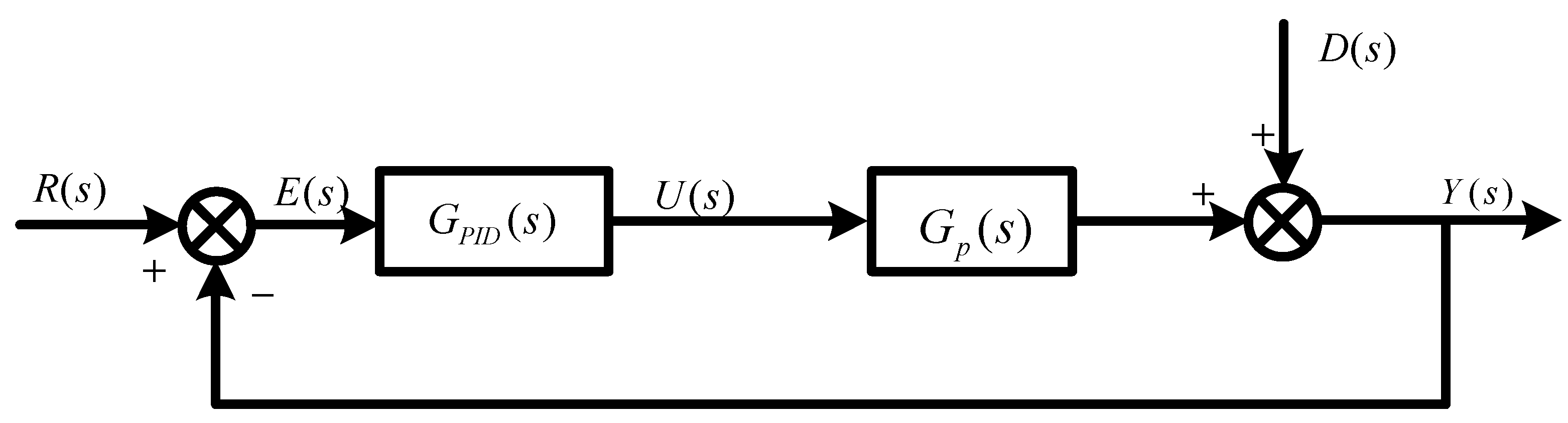
Figure 1.
Schematic diagram of the proportion integration differentiation (PID) control system.
Figure 1.
Schematic diagram of the proportion integration differentiation (PID) control system.
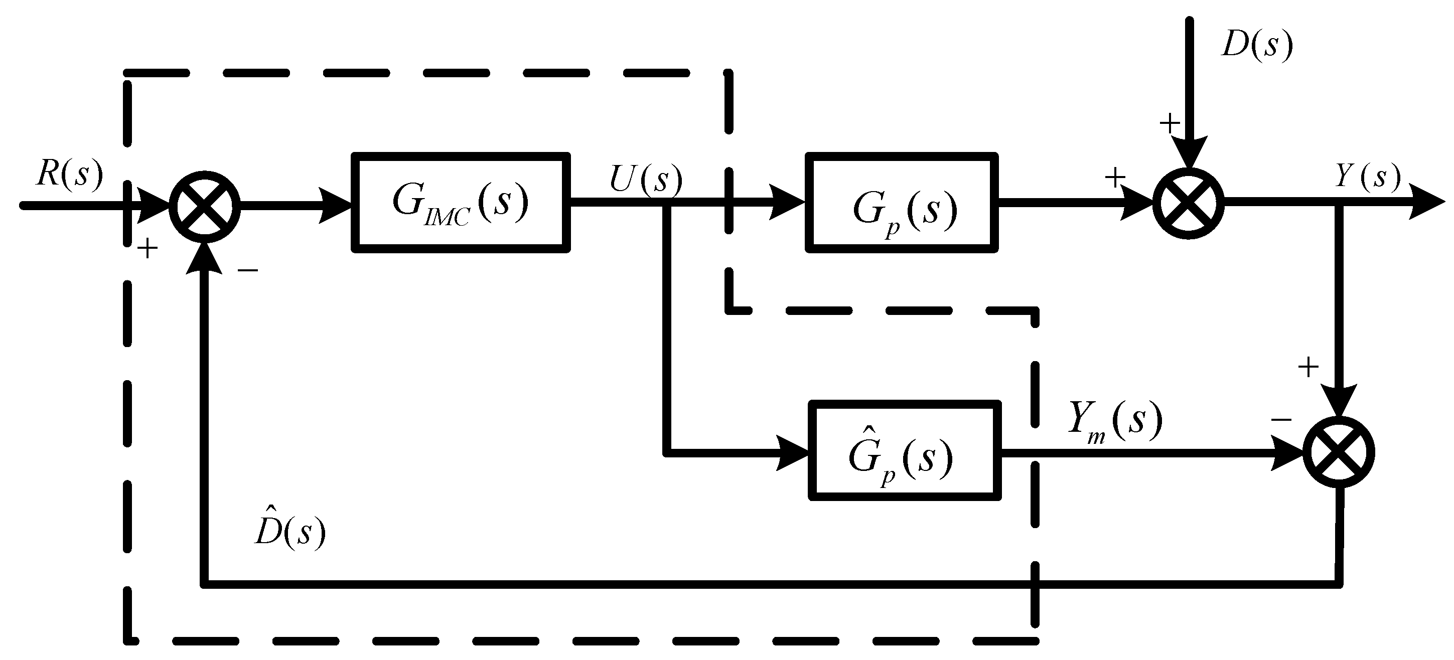
Figure 2.
Schematic diagram of the internal model control (IMC) system.
Figure 2.
Schematic diagram of the internal model control (IMC) system.
Figure 3.
Production flow chart of the thermal power unit.
Figure 3.
Production flow chart of the thermal power unit.
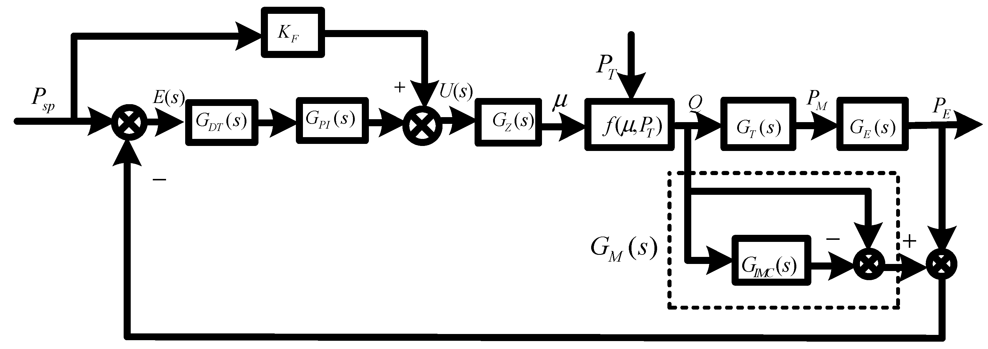
Figure 4.
Schematic diagram of power control system (PCS) based on proportional integral (PI) plus feed forward (FF) (Psp—power reference value; E(s)—error; U(s)—controller output; μ—valve opening; PT—main steam pressure; Q—steam flow; PM—mechanical power; PE—electromagnetic power; KF—FF gain; GPI(s)—controller; GZ(s)—actuator; f(μ,PT)—function; GT(s)—steam turbine; GE(s)—generator).
Figure 5.
Schematic diagram of the power control system (PCS) based on IMC-PI (
GDT(
s)—low pass filter;
GM(
s)—built-in model;
GIMC(
s)—transfer function of
Q and
PM. (the remaining components are the same as in
Figure 4)).
Figure 5.
Schematic diagram of the power control system (PCS) based on IMC-PI (
GDT(
s)—low pass filter;
GM(
s)—built-in model;
GIMC(
s)—transfer function of
Q and
PM. (the remaining components are the same as in
Figure 4)).
Figure 6.
Schematic diagram of PCS based on IMC-PI plus FF. (Please refer to the corresponding components in
Figure 4 and
Figure 5).
Figure 6.
Schematic diagram of PCS based on IMC-PI plus FF. (Please refer to the corresponding components in
Figure 4 and
Figure 5).
Figure 7.
Generator power responses of the actual model and a simplified model.
Figure 7.
Generator power responses of the actual model and a simplified model.
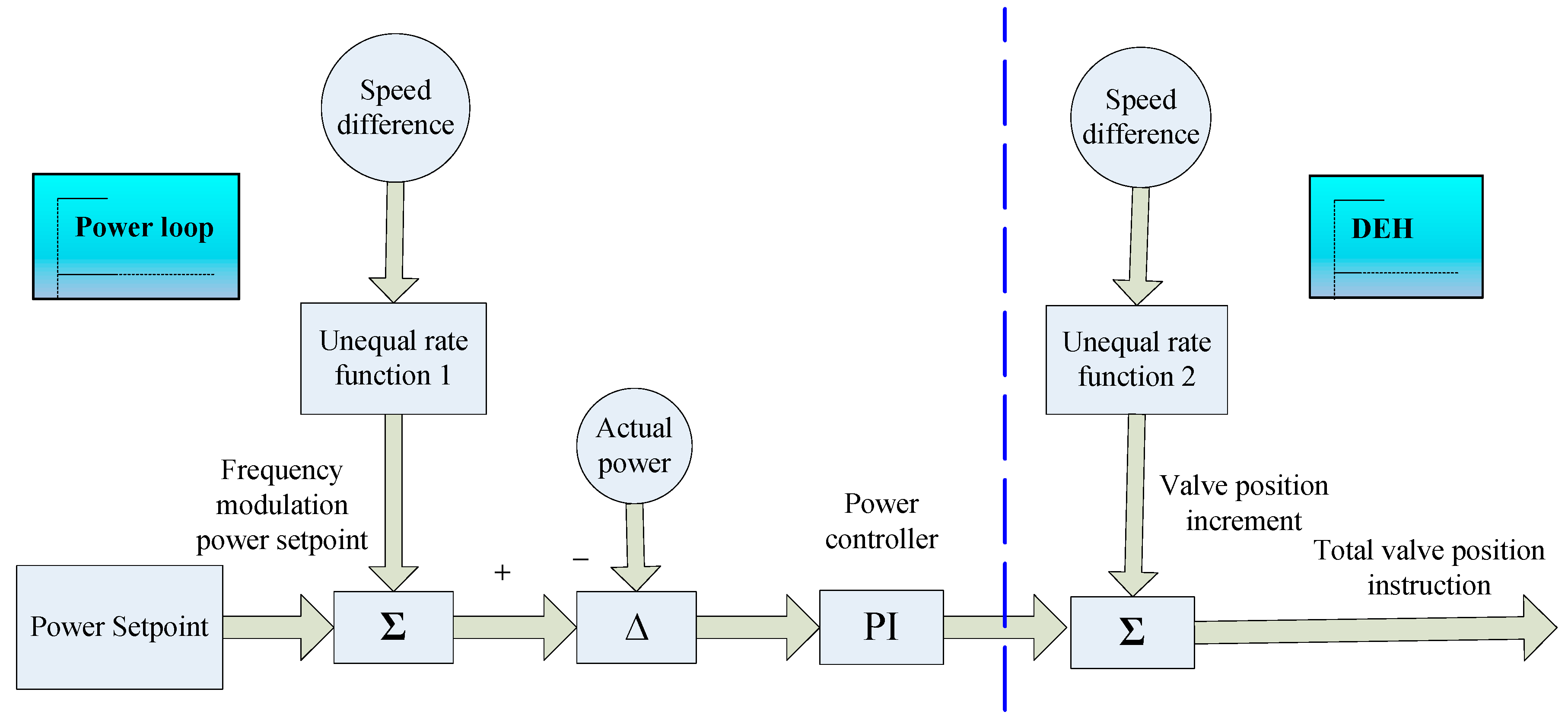
Figure 8.
Typical schematic diagram of primary frequency modulation (PFM) of thermal power unit (DEH: Digital Electro-hydraulic Control).
Figure 8.
Typical schematic diagram of primary frequency modulation (PFM) of thermal power unit (DEH: Digital Electro-hydraulic Control).
Figure 9.
Rotational speed inequality curve.
Figure 9.
Rotational speed inequality curve.
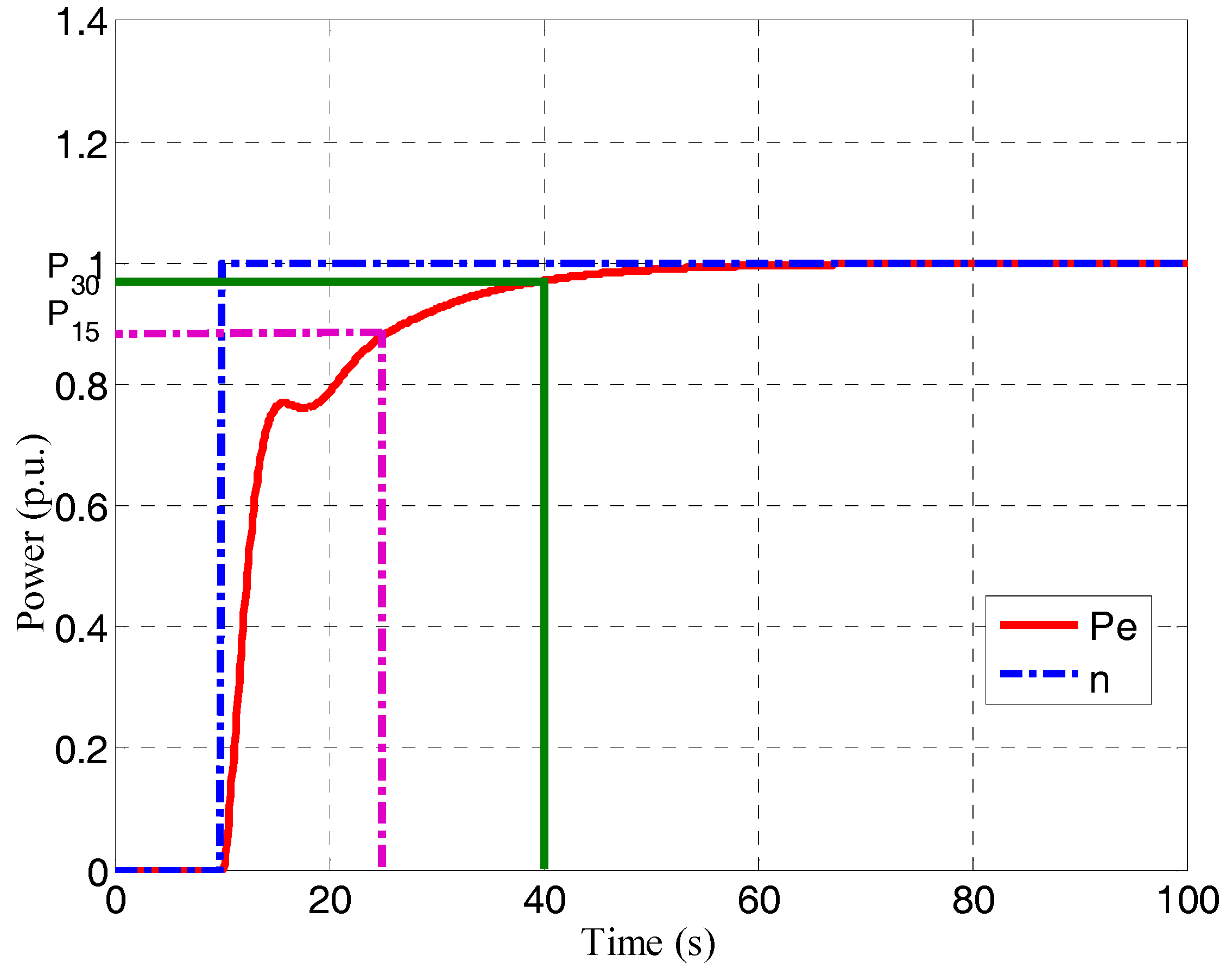
Figure 10.
Typical power response curve.
Figure 10.
Typical power response curve.
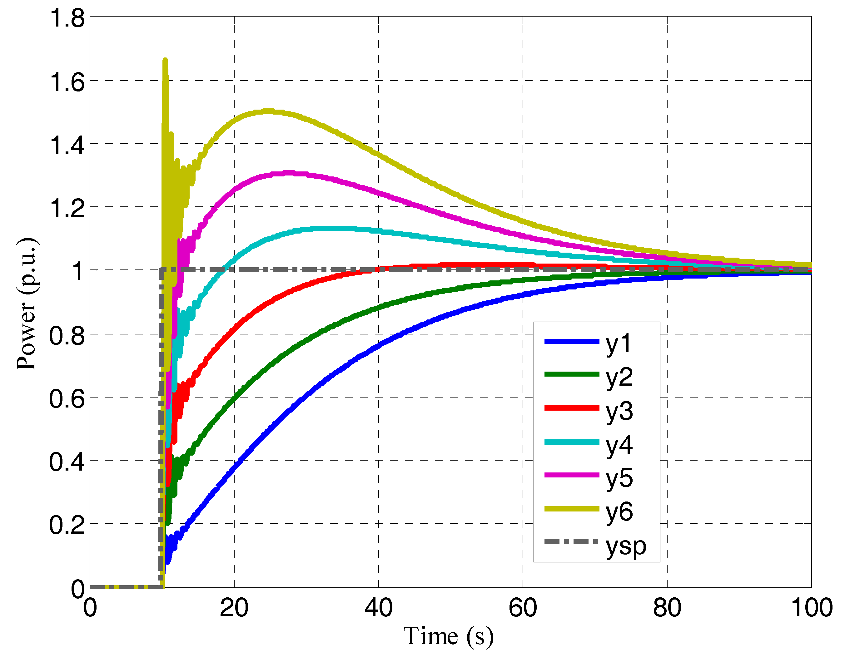
Figure 11.
The response of PCS with different FF coefficients.
Figure 11.
The response of PCS with different FF coefficients.
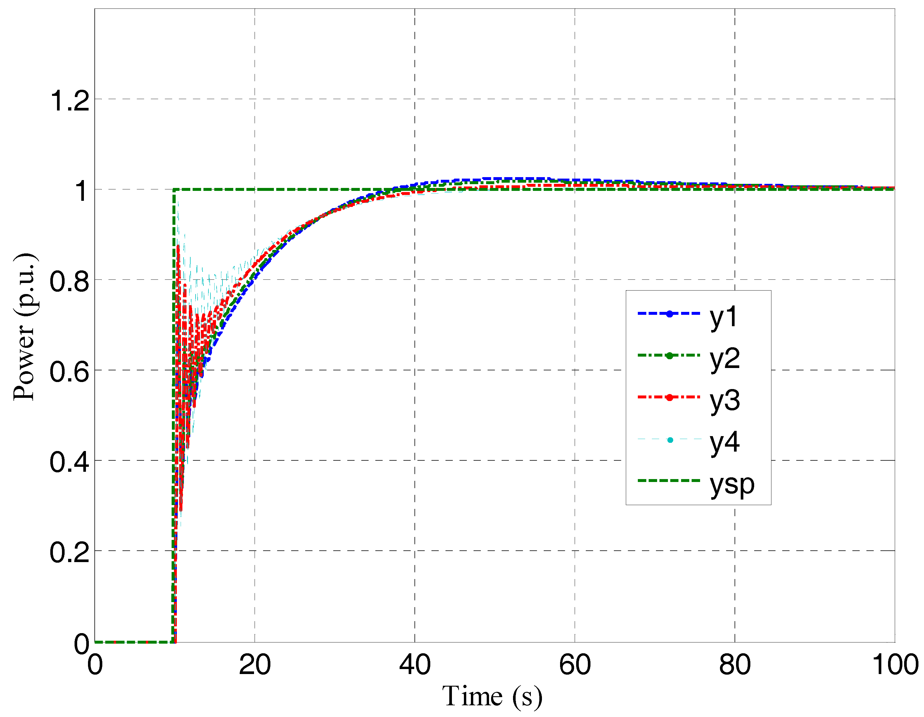
Figure 12.
PCS response with different proportional gain.
Figure 12.
PCS response with different proportional gain.
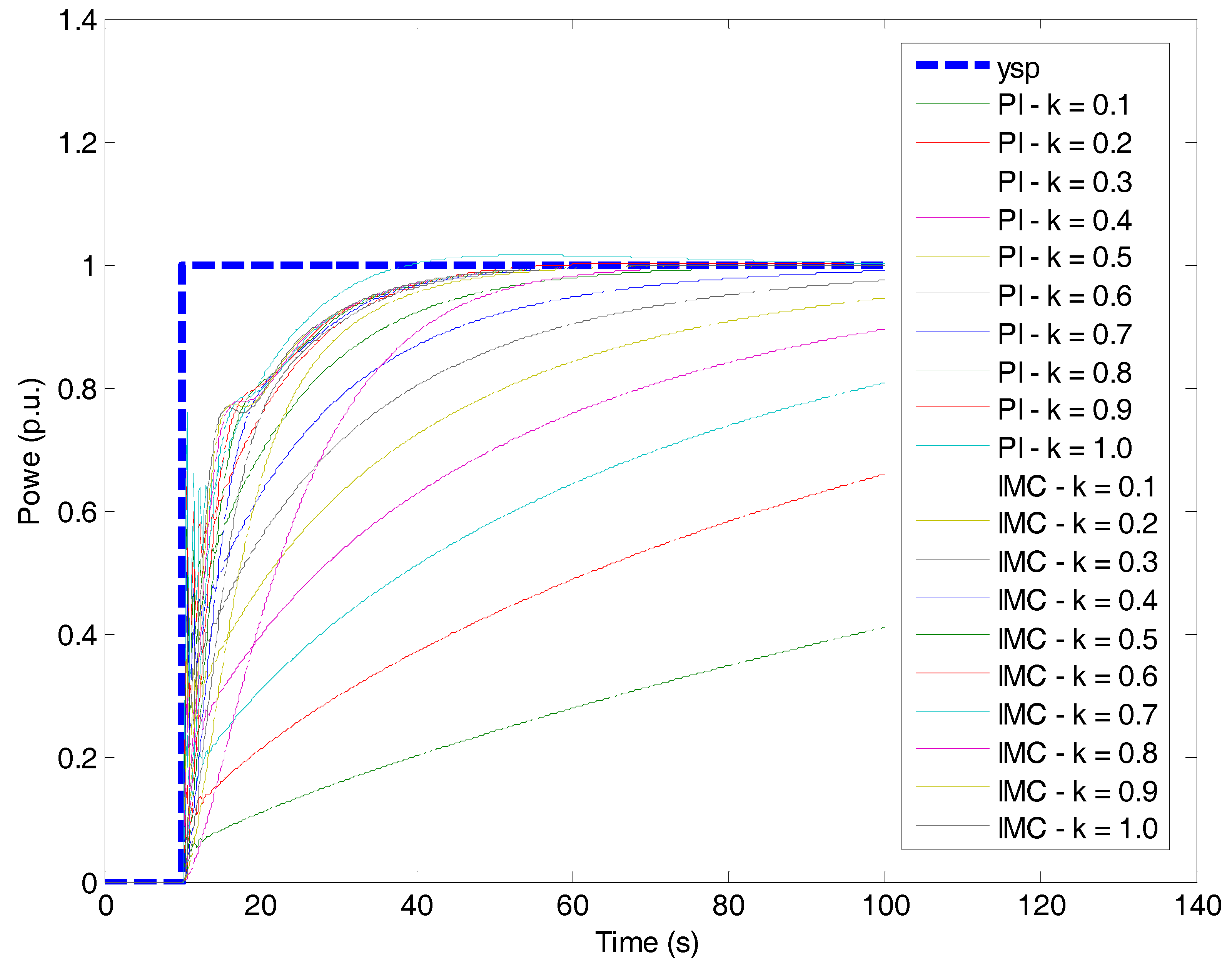
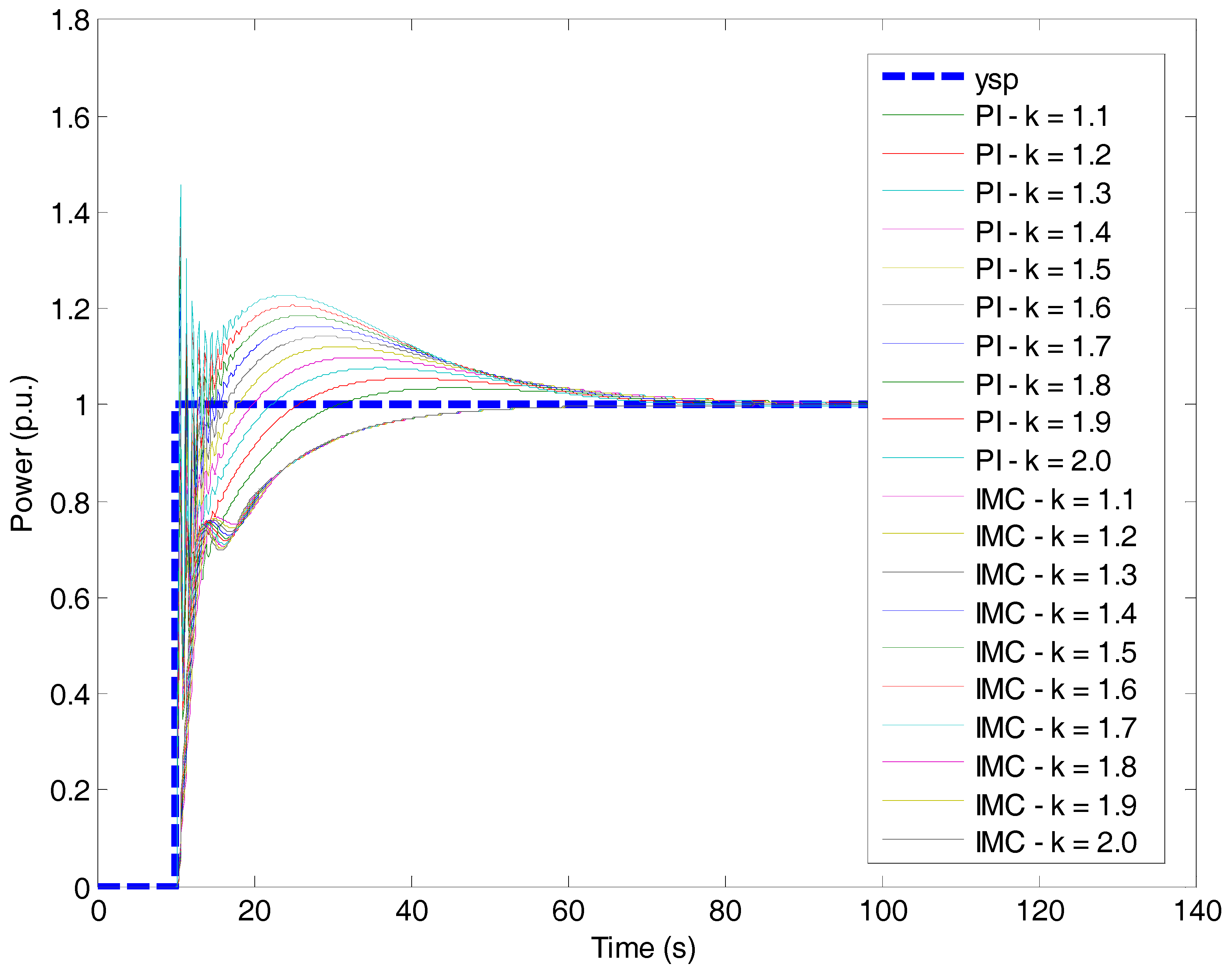
Figure 13.
Oscillatory output of PCS.
Figure 13.
Oscillatory output of PCS.
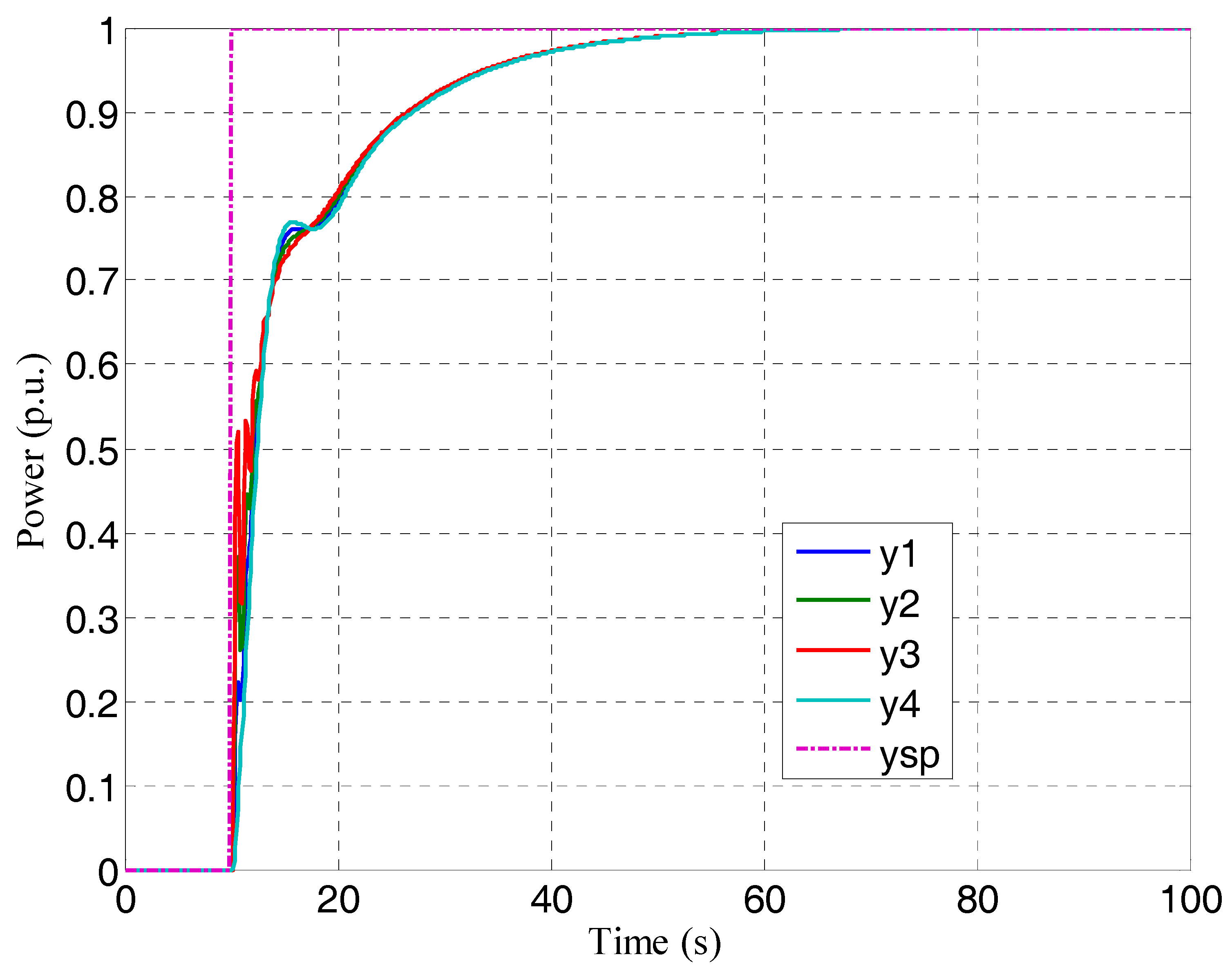
Figure 14.
PCS response with different integral gains.
Figure 14.
PCS response with different integral gains.
Figure 15.
PCS response with four different IMC-PI parameters.
Figure 15.
PCS response with four different IMC-PI parameters.
Figure 16.
The power response of IMC-PI plus different FF coefficient.
Figure 16.
The power response of IMC-PI plus different FF coefficient.
Figure 17.
The relationship between and .
Figure 17.
The relationship between and .
Figure 18.
The relationship between and .
Figure 18.
The relationship between and .
Figure 19.
The relationship between and .
Figure 19.
The relationship between and .
Figure 20.
The relationship between and .
Figure 20.
The relationship between and .
Figure 21.
The relationship between and .
Figure 21.
The relationship between and .
Figure 22.
The relationship between and .
Figure 22.
The relationship between and .
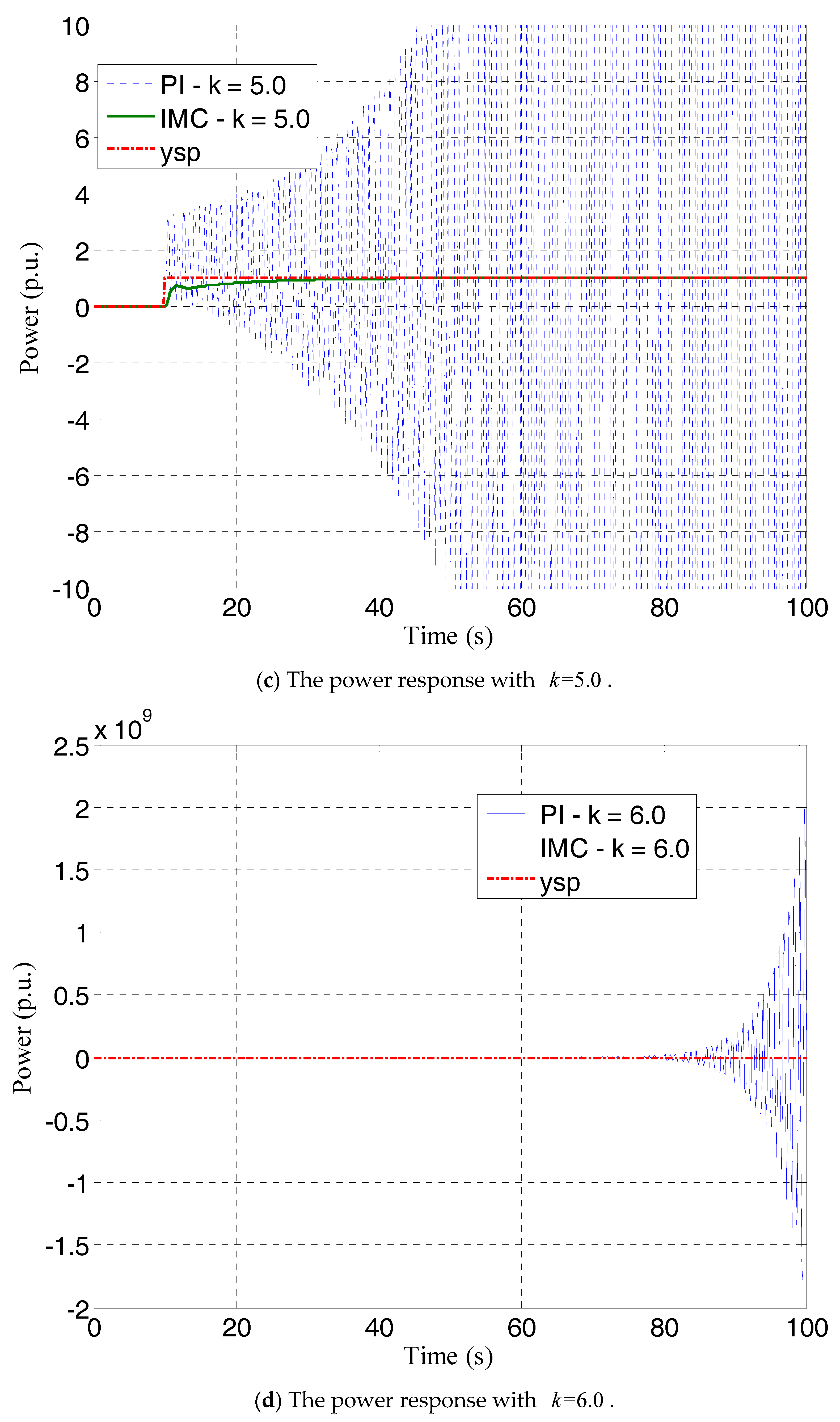
Figure 23.
The power response with .
Figure 23.
The power response with .
Figure 24.
The power response with .
Figure 24.
The power response with .
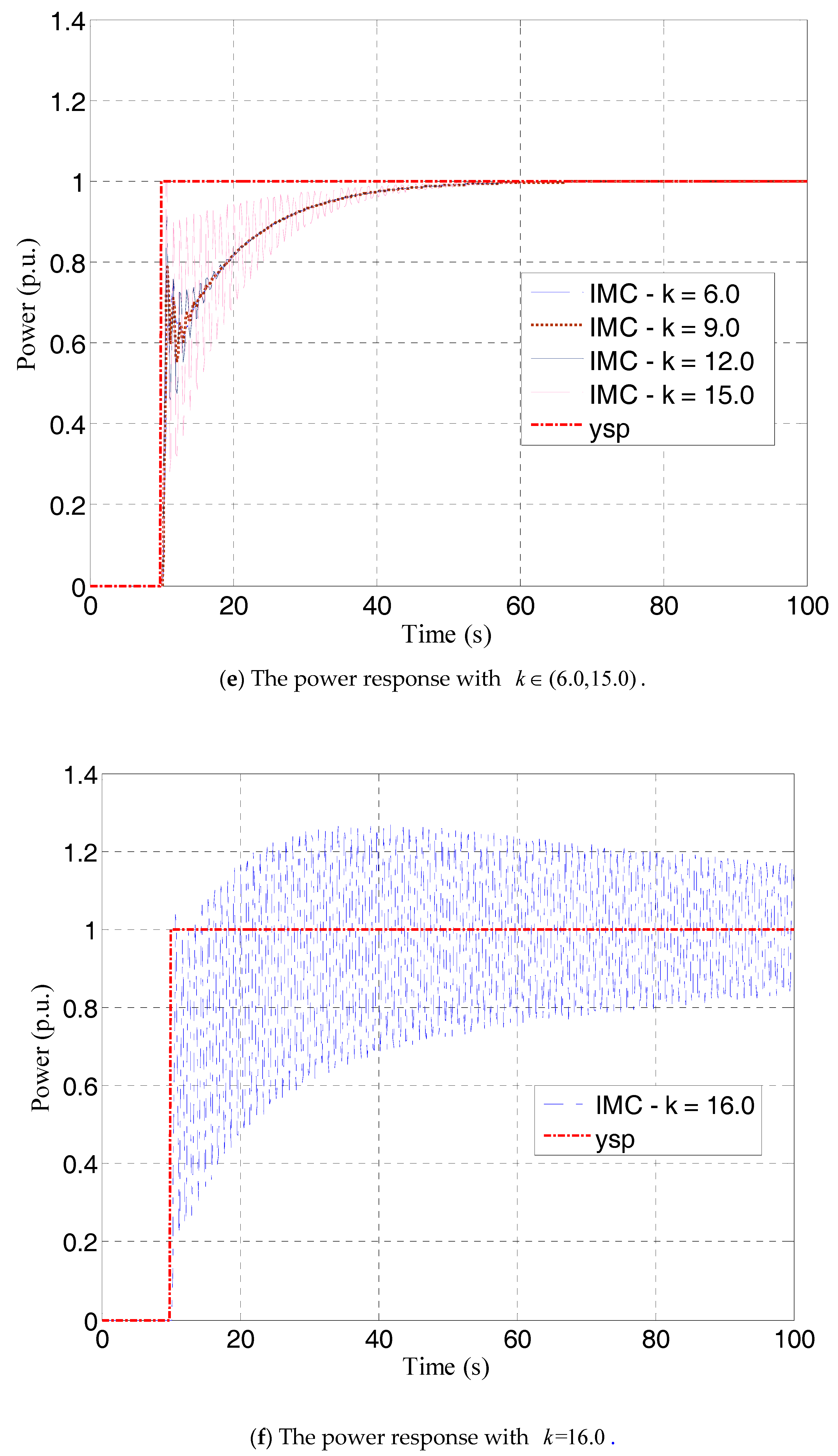
Figure 25.
The power response with .
Figure 25.
The power response with .
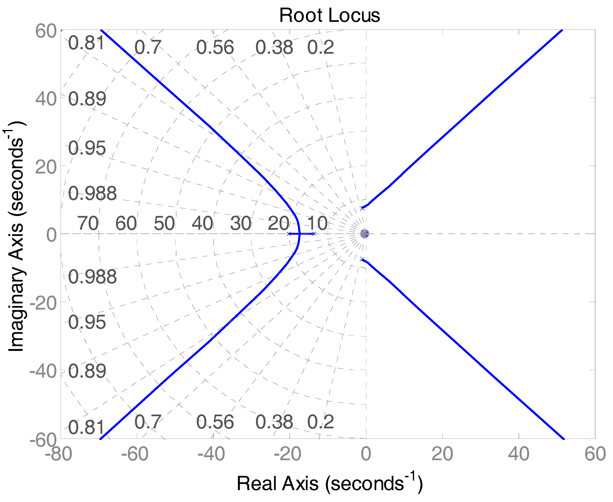
Figure 26.
Root locus of system based on PI-FF.
Figure 26.
Root locus of system based on PI-FF.
Figure 27.
Root locus of system based on IMC-PI.
Figure 27.
Root locus of system based on IMC-PI.
Table 1.
The controller parameters under two control modes (PI: Proportion Integration; FF: Feed forward; IMC: Internal model control).
Table 1.
The controller parameters under two control modes (PI: Proportion Integration; FF: Feed forward; IMC: Internal model control).
| PI + FF | IMC + PI |
|---|
|
#
## |
Table 2.
Dynamic performance indexes and qualified scope of the power control system (PCS).
Table 2.
Dynamic performance indexes and qualified scope of the power control system (PCS).
| Performance Dynamic Index | Qualified Scope |
|---|
| |
| |
| |
| |
Table 3.
Benchmark and result of dynamic performance assessment for the PCS (: Dynamic Performance Assessment Index).
Table 3.
Benchmark and result of dynamic performance assessment for the PCS (: Dynamic Performance Assessment Index).
| | Performance Assessment Results |
|---|
| | Excellent |
| | Good |
| | Medium |
| 1 | Poor |
| 0 | So Bad |
| System Unstable | 0 | Unacceptable |
Table 4.
Performance result of primary frequency modulation (PFM) with different controllers.
Table 4.
Performance result of primary frequency modulation (PFM) with different controllers.
| KF | Output | | | | | | Num | Performance |
|---|
| 0 | y1 | 49.52 | 75.88 | 72.10 | 70.08 | 0.9232 | 1 | Poor |
| 0.4 | y2 | 69.66 | 88.05 | 56.50 | 78.02 | 1.1195 | 2 | Medium |
| 0.8 | y3 | 89.79 | 100.22 | 24.20 | 85.95 | 1.6126 | 4 | Excellent |
| 1.2 | y4 | 109.93 | 112.39 | 72.80 | 93.88 | 1.3376 | 3 | Good |
| 1.6 | y5 | 130.06 | 124.56 | 81.50 | 101.80 | 1.4544 | 3 | Good |
| 2.0 | y6 | 150.20 | 136.73 | 86.80 | 109.80 | 1.5823 | 3 | Good |
Table 5.
Performance results of PFM with different controllers.
Table 5.
Performance results of PFM with different controllers.
| Controller | Output | | | | | | Num | Performance |
|---|
| y1 | 89.40 | 100.88 | 50.80 | 85.96 | 1.2885 | 4 | Medium |
| y2 | 89.79 | 100.22 | 24.20 | 85.95 | 1.6126 | 4 | Excellent |
| y3 | 90.51 | 99.25 | 25.80 | 85.95 | 1.5740 | 4 | Excellent |
| y4 | 90.97 | 98.61 | 27.40 | 85.97 | 1.5400 | 4 | Excellent |
Table 6.
Performance result of PFM with different controllers.
Table 6.
Performance result of PFM with different controllers.
| Controller | Output | | | | | | Num | Performance |
|---|
| y1 | 79.11 | 87.37 | 223.80 | 77.37 | 0.9475 | 1 | Poor |
| y2 | 82.18 | 91.83 | 88.30 | 81.06 | 1.0908 | 3 | Medium |
| y3 | 84.96 | 95.35 | 42.30 | 83.41 | 1.3058 | 4 | Good |
| y4 | 87.49 | 98.10 | 29.70 | 84.94 | 1.4795 | 4 | Good |
| y5 | 89.79 | 100.22 | 24.20 | 85.95 | 1.6126 | 4 | Excellent |
| y6 | 91.87 | 101.82 | 49.70 | 86.65 | 1.3399 | 4 | Good |
Table 7.
Performance result of PFM with four different controllers.
Table 7.
Performance result of PFM with four different controllers.
| Controller | Output | | | | | | Num | Performance |
|---|
| # | y1 | 87.83 | 97.08 | 33.90 | 84.01 | 1.4108 | 4 | Good |
| # | y2 | 78.28 | 87.40 | 87.80 | 78.69 | 1.0552 | 2 | Poor |
| # | y3 | 42.56 | 68.81 | 92.00 | 65.49 | 0.8134 | 1 | Poor |
| # | y4 | 41.27 | 64.84 | 138.00 | 61.75 | 0.7256 | 1 | Poor |
Table 8.
Performance result under IMC-PI with different FF coefficients.
Table 8.
Performance result under IMC-PI with different FF coefficients.
| KF | Output | | | | | | Num | Performance |
|---|
| 0.00 | y1 | 87.83 | 97.08 | 33.90 | 84.01 | 1.4108 | 4 | Good |
| 0.20 | y2 | 87.99 | 97.13 | 33.90 | 84.21 | 1.4124 | 4 | Good |
| 0.40 | y3 | 88.15 | 97.18 | 33.90 | 84.41 | 1.4141 | 4 | Good |
| 0.60 | y4 | 88.30 | 97.23 | 33.90 | 84.61 | 1.4157 | 4 | Good |
Table 9.
Test data and local valve flow coefficients in sequence valve mode.
Table 9.
Test data and local valve flow coefficients in sequence valve mode.
| | | |
|---|
| 68.00 | 184.40 | 61.47 | - |
| 68.60 | 199.60 | 66.53 | 8.433 |
| 70.10 | 255.30 | 75.10 | 5.713 |
| 72.10 | 237.00 | 79.00 | 1.950 |
| 75.10 | 241.90 | 80.63 | 0.543 |
| 79.10 | 247.30 | 82.43 | 0.450 |
| 81.10 | 246.40 | 82.13 | −0.150 |
| 83.10 | 247.30 | 82.43 | 0.150 |
| 87.10 | 257.70 | 85.90 | 0.868 |
| 88.50 | 280.40 | 93.47 | 5.407 |
| 92.50 | 284.60 | 94.87 | 0.350 |
| 97.00 | 287.20 | 95.73 | 0.191 |
| 99.00 | 290.00 | 96.67 | 0.470 |
| 100.00 | 294.20 | 98.07 | 1.400 |
Table 10.
Test data and local valve flow coefficients in single valve mode.
Table 10.
Test data and local valve flow coefficients in single valve mode.
| | | Local Flow |
|---|
| 86.00 | 182.50 | 60.83 | - |
| 87.00 | 186.00 | 62.00 | 1.170 |
| 88.00 | 192.00 | 64.00 | 2.000 |
| 89.00 | 198.50 | 66.17 | 2.170 |
| 90.00 | 202.80 | 67.60 | 1.430 |
| 90.50 | 205.50 | 68.50 | 1.800 |
| 91.00 | 209.00 | 69.67 | 2.340 |
| 91.50 | 220.20 | 73.40 | 7.460 |
| 92.00 | 228.40 | 76.13 | 5.460 |
| 92.50 | 242.00 | 80.67 | 9.080 |
| 93.00 | 248.90 | 82.97 | 4.600 |
| 94.00 | 260.10 | 86.70 | 3.730 |
| 95.00 | 265.10 | 88.37 | 1.670 |
| 96.00 | 273.80 | 91.27 | 2.900 |
| 97.00 | 283.60 | 94.53 | 3.260 |
| 98.00 | 286.80 | 95.60 | 1.070 |
| 100.00 | 296.10 | 98.70 | 1.550 |
Table 11.
The performance result with .
Table 11.
The performance result with .
| PI plus FF Control |
|---|
| | | | | Num | Performance |
|---|
| 0.10 | 13.63 | 20.33 | 761.70 | 22.82 | 0.2327 | 0 | So Bad |
| 0.20 | 25.93 | 37.19 | 369.10 | 39.47 | 0.4223 | 0 | So Bad |
| 0.30 | 37.01 | 51.18 | 236.90 | 51.79 | 0.5803 | 1 | Poor |
| 0.40 | 47.02 | 62.77 | 169.40 | 61.01 | 0.7155 | 1 | Poor |
| 0.50 | 56.06 | 72.37 | 127.40 | 68.03 | 0.8352 | 1 | Poor |
| 0.60 | 64.23 | 80.30 | 97.20 | 73.44 | 0.9469 | 1 | Poor |
| 0.70 | 71.61 | 86.84 | 72.60 | 77.67 | 1.0622 | 1 | Poor |
| 0.80 | 78.29 | 92.22 | 50.80 | 81.04 | 1.2041 | 2 | Medium |
| 0.90 | 84.33 | 96.62 | 34.20 | 83.74 | 1.3927 | 4 | Good |
| 1.00 | 89.79 | 100.22 | 34.20 | 85.95 | 1.4314 | 4 | Excellent |
Table 12.
The performance result with .
Table 12.
The performance result with .
| IMC-PI Control |
|---|
| | | | | Num | Performance |
|---|
| 0.10 | 60.75 | 88.96 | 49.00 | 75.01 | 1.1178 | 2 | Medium |
| 0.20 | 80.40 | 95.50 | 38.50 | 80.01 | 1.3090 | 4 | Good |
| 0.30 | 85.29 | 96.31 | 36.30 | 81.67 | 1.3593 | 4 | Good |
| 0.40 | 85.97 | 96.64 | 35.40 | 82.51 | 1.3772 | 4 | Good |
| 0.50 | 86.03 | 96.80 | 34.90 | 83.01 | 1.3864 | 4 | Good |
| 0.60 | 86.31 | 96.90 | 34.60 | 83.34 | 1.3929 | 4 | Good |
| 0.70 | 86.78 | 96.97 | 34.30 | 83.58 | 1.3997 | 4 | Good |
| 0.80 | 87.26 | 97.02 | 34.20 | 83.76 | 1.4036 | 4 | Excellent |
| 0.90 | 87.62 | 97.05 | 34.00 | 83.90 | 1.4081 | 4 | Excellent |
| 1.00 | 87.83 | 97.08 | 33.90 | 84.01 | 1.4108 | 4 | Excellent |
Table 13.
The performance result with .
Table 13.
The performance result with .
| PI plus FF Control |
|---|
| | | | | Num | Performance |
|---|
| 1.10 | 94.74 | 103.14 | 55.60 | 87.78 | 1.2959 | 4 | Good |
| 1.20 | 99.21 | 105.49 | 58.50 | 89.31 | 1.3113 | 4 | Good |
| 1.30 | 103.27 | 107.36 | 58.90 | 90.60 | 1.3344 | 4 | Good |
| 1.40 | 106.93 | 108.84 | 58.30 | 91.71 | 1.3587 | 4 | Good |
| 1.50 | 110.25 | 109.99 | 57.40 | 92.67 | 1.3816 | 4 | Good |
| 1.60 | 113.26 | 110.86 | 56.20 | 93.51 | 1.4037 | 4 | Excellent |
| 1.70 | 115.97 | 111.50 | 55.00 | 94.25 | 1.4240 | 4 | Excellent |
| 1.80 | 118.43 | 111.95 | 53.80 | 94.90 | 1.4427 | 4 | Excellent |
| 1.90 | 120.65 | 112.25 | 52.60 | 95.49 | 1.4602 | 4 | Excellent |
| 2.00 | 122.66 | 112.41 | 51.40 | 96.01 | 1.4766 | 4 | Excellent |
Table 14.
The performance result with .
Table 14.
The performance result with .
| IMC-PI Control |
|---|
| | | | | Num | Performance |
|---|
| 1.10 | 87.93 | 97.11 | 33.90 | 84.10 | 1.4116 | 4 | Excellent |
| 1.20 | 87.94 | 97.13 | 33.80 | 84.17 | 1.4134 | 4 | Excellent |
| 1.30 | 87.92 | 97.14 | 33.70 | 84.24 | 1.4150 | 4 | Excellent |
| 1.40 | 87.90 | 97.16 | 32.70 | 84.29 | 1.4288 | 4 | Excellent |
| 1.50 | 87.90 | 97.17 | 33.60 | 84.34 | 1.4168 | 4 | Excellent |
| 1.60 | 87.92 | 97.18 | 33.60 | 84.38 | 1.4171 | 4 | Excellent |
| 1.70 | 87.95 | 97.17 | 33.60 | 84.42 | 1.4174 | 4 | Excellent |
| 1.80 | 88.00 | 97.19 | 33.50 | 84.45 | 1.4191 | 4 | Excellent |
| 1.90 | 88.05 | 97.20 | 33.50 | 84.48 | 1.4195 | 4 | Excellent |
| 2.00 | 88.10 | 97.21 | 33.50 | 84.51 | 1.4198 | 4 | Excellent |
Table 15.
The performance result with .
Table 15.
The performance result with .
| PI plus FF Control |
|---|
| | | | | Num | Performance |
|---|
| 3.00 | 133.84 | 110.55 | 42.60 | 99.34 | 1.5859 | 4 | Excellent |
| 4.00 | 152.28 | 108.44 | 38.60 | 101.00 | 1.6866 | 4 | Excellent |
| 5.00 | ——※ | ——※ | ——※ | ——※ | ——※ | 0 | Unacceptable |
| 6.00 | ——※ | ——※ | ——※ | ——※ | ——※ | 0 | Unacceptable |
| 7.00 | ——※ | ——※ | ——※ | ——※ | ——※ | 0 | Unacceptable |
| 8.00 | ——※ | ——※ | ——※ | ——※ | ——※ | 0 | Unacceptable |
| 9.00 | ——※ | ——※ | ——※ | ——※ | ——※ | 0 | Unacceptable |
| 10.00 | ——※ | ——※ | ——※ | ——※ | ——※ | 0 | Unacceptable |
| 12.00 | ——※ | ——※ | ——※ | ——※ | ——※ | 0 | Unacceptable |
| 15.00 | ——※ | ——※ | ——※ | ——※ | ——※ | 0 | Unacceptable |
| 16.00 | ——※ | ——※ | ——※ | ——※ | ——※ | 0 | Unacceptable |
Table 16.
The performance result with .
Table 16.
The performance result with .
| IMC-PI Control |
|---|
| | | | | Num | Performance |
|---|
| 3.00 | 88.29 | 97.25 | 33.30 | 84.67 | 1.4240 | 4 | Excellent |
| 4.00 | 88.37 | 97.27 | 33.30 | 84.76 | 1.4248 | 4 | Excellent |
| 5.00 | 88.42 | 97.28 | 33.20 | 84.81 | 1.4266 | 4 | Excellent |
| 6.00 | 88.45 | 97.28 | 33.20 | 84.84 | 1.4268 | 4 | Excellent |
| 7.00 | 88.47 | 97.29 | 33.20 | 84.86 | 1.4270 | 4 | Excellent |
| 8.00 | 88.49 | 97.29 | 33.20 | 84.88 | 1.4272 | 4 | Excellent |
| 9.00 | 88.50 | 97.30 | 33.10 | 84.90 | 1.4287 | 4 | Excellent |
| 10.00 | 88.51 | 97.30 | 33.10 | 84.91 | 1.4288 | 4 | Excellent |
| 12.00 | 88.56 | 97.30 | 33.10 | 84.92 | 1.4290 | 4 | Excellent |
| 15.00 | 95.14 | 98.65 | 37.10 | 84.94 | 1.4058 | 4 | Excellent |
| 16.00 | ——※ | ——※ | ——※ | ——※ | ——※ | 0 | Unacceptable |


