Mathematical Modeling of RBC Count Dynamics after Blood Loss

 and
and
Abstract
:1. Introduction
1.1. Overview of Erythropoiesis
1.2. History of Erythropoiesis Modeling and Comparison with Our Approach
1.3. Motivating Practical Application: Polycythemia Vera
2. Model
2.1. Assumptions on the Subject
- Healthy adult subject: The aim of the proposed model is to describe the RBC dynamics of healthy adult subjects. Healthy in this case especially means that the subject has no disturbed erythropoiesis as for example in the case of PV.
- Existence of a steady state: It is assumed that environmental conditions that affect the blood do not dramatically change. If this is the case, a mean value for the erythrocyte count should exist in healthy individuals, which is valid over a longer time period. This will be the value of the system and the steady state for the erythrocyte count in the model. Using this assumption especially means that the model will not be able to capture large environmental effects to the blood.
- Sufficient iron concentration: The iron concentration in considered individuals is assumed to be sufficient, such that erythropoiesis is not affected by iron shortage. Therefore, iron influence on erythropoiesis is not included in the model.
- Reasonable blood loss: It is assumed that the blood loss in the considered subjects does not exceed a standard blood donation by much. Therefore, emergency reactions of the body in case of severe anemia (for example the release of stress reticulocyte, compare [2]) should not arise and are therefore not included in this model.
2.2. Assumptions on the Physiological Process
- 5.
- Average cell: A compartment modeling approach is used to describe the system dynamics. Therefore, all cells in one compartment share the same properties given by the mean values of the corresponding properties. On the one hand, cell individual information like cell age is lost, which leads to errors especially in early phases where proliferation is very dependent on the state of the cell. On the other hand, often only summarized properties like for example amount of cells or overall amount of hemoglobin is interesting for our application. In addition, influences in early cell stages are often not measured in clinical practice, such that an error in early cell stages is not preventable. The assumption that given mean values reflect summarized properties is justified, as there is a very large number of cells in each compartment and the law of large numbers can be applied.
- 6.
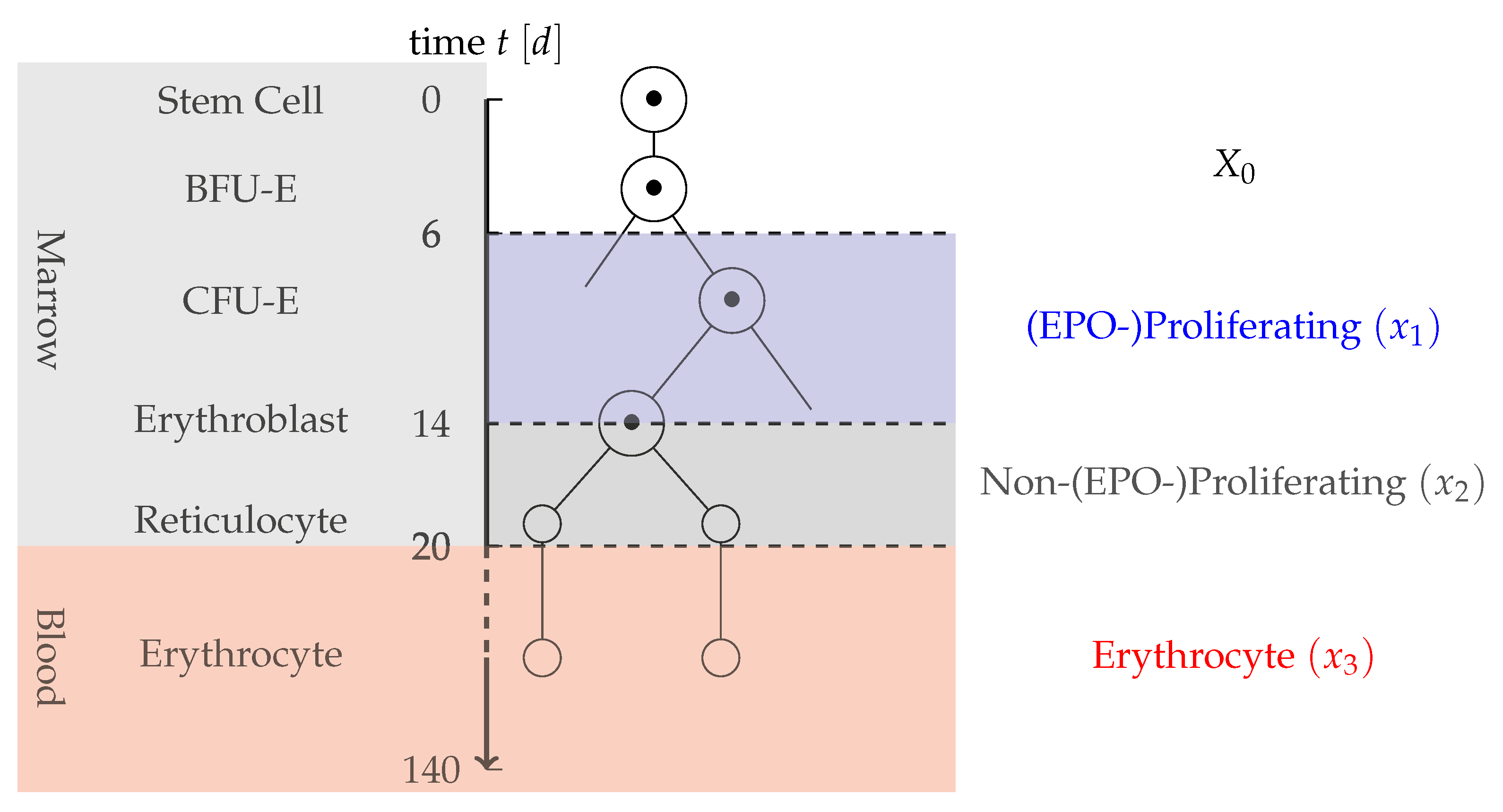
- Partition of progenitor cells: Measurements only include information on the mature RBC and not on previous cell stages. Therefore, in the application oriented model, a too detailed differentiation of early stem cells should be prevented. As EPO is the main factor for compensation of a blood loss, a partition into two cell types is proposed: cells that are strongly proliferating in dependence on EPO and cells that are not or only slightly affected by EPO. Cells strongly affected by EPO here include CFU-E cells and early erythroblasts. Not affected or less affected by EPO are BFU-E, later erythroblasts and reticulocytes. As BFU-E are not affected by the dynamics, they are modeled by a constant inflow term , whereas the EPO-depending and Non-EPO-depending cells are each described by one compartment. The partition of erythropoiesis can be examined in Figure 1.
- 7.
- Instant blood plasma regeneration: After a blood loss, both solid and liquid blood components are lost. It is known that blood plasma regenerates very fast after about two to four days [23]. To prevent the usage of delay components in the model, it is here assumed that the regeneration of blood plasma is instant after a reasonable blood loss. This error should be low, as the horizon of about three days is small compared to the average time after a blood donation of about 42 days.
- 8.
- Instant feedback by EPO: The EPO production in the human body is adapted to a changing demand for erythrocytes. This process does not instantaneously change the production rate of erythrocytes, as it takes a while for the local EPO production in, for example, the liver to change the overall concentration of EPO. For our modeling approach, it is assumed that this process is instantaneous. This error also should be low, as the observed time scale is very large.
- 9.
- Implicit feedback by EPO: As stated in Section 1.1, EPO is mainly responsible for the regeneration of RBCs after changing hemoglobin concentrations for example due to blood loss. Unfortunately, EPO concentrations fluctuate strongly on a small time scale and are difficult to measure in clinical practice. Therefore, no direct information about EPO concentration in the subject is available [24]. The influence of EPO on erythropoiesis is therefore indirectly described by a negative feedback term based on the fractional blood loss.We assume the feedback function to be linear, which is certainly valid for small variations in RBC counts. This assumption may however be violated for larger amounts of blood loss and pathological cases, as discussed in Section 5.
- 10.
- Only most necessary processes: To reduce the model complexity, only the most essential features of erythropoiesis after blood loss are included. Therefore, processes like neocytolysis [2], which has a minor influence on young erythrocytes, is not included.
- 11.
- No self-renewal of progenitor cells: It is known that stem cells, especially those that are not committed to a hematopoetic lineage, have the capability of self-renewal to maintain the population of cells. The capability of self-renewal decreases with increased maturation progress [2]. There exist mathematical models that consider self-renewal to be even present in progenitor cells (see for example [25]). In contrast to that, here it is assumed that in the considered progenitor cell compartments only differentiation and no self-renewal is present.
- 12.
- Transport rates of cells: In case of severe anemia, cells might have an increased differentiation rate induced by high EPO concentrations to compensate for the lack of cells [2]. Due to Assumption 4, those reactions do not have to be considered here. Therefore, it is assumed that cells have a constant differentiation rate concerning EPO. Based on [2], it can be assumed that the EPO-Proliferating phase and the Non-EPO-Proliferating phase have an average duration of eight and six days, respectively. The transport rates and are set to the respective reciprocal values. As the average lifespan of a mature erythrocyte can be assumed to be 120 days, the death rate for the erythrocyte compartment is set to .
- 13.
- Individual features of erythropoiesis: Between individuals, there might be a strong variation in the pace of erythropoiesis. For example, a large individual often has more blood than a small individual and therefore should have a faster erythropoiesis to cover for example for fractional cell loss due to cell senescence. This is covered by two amplification variables: for the overall cell maturation and for the reaction to a blood loss.
2.3. Model Equations
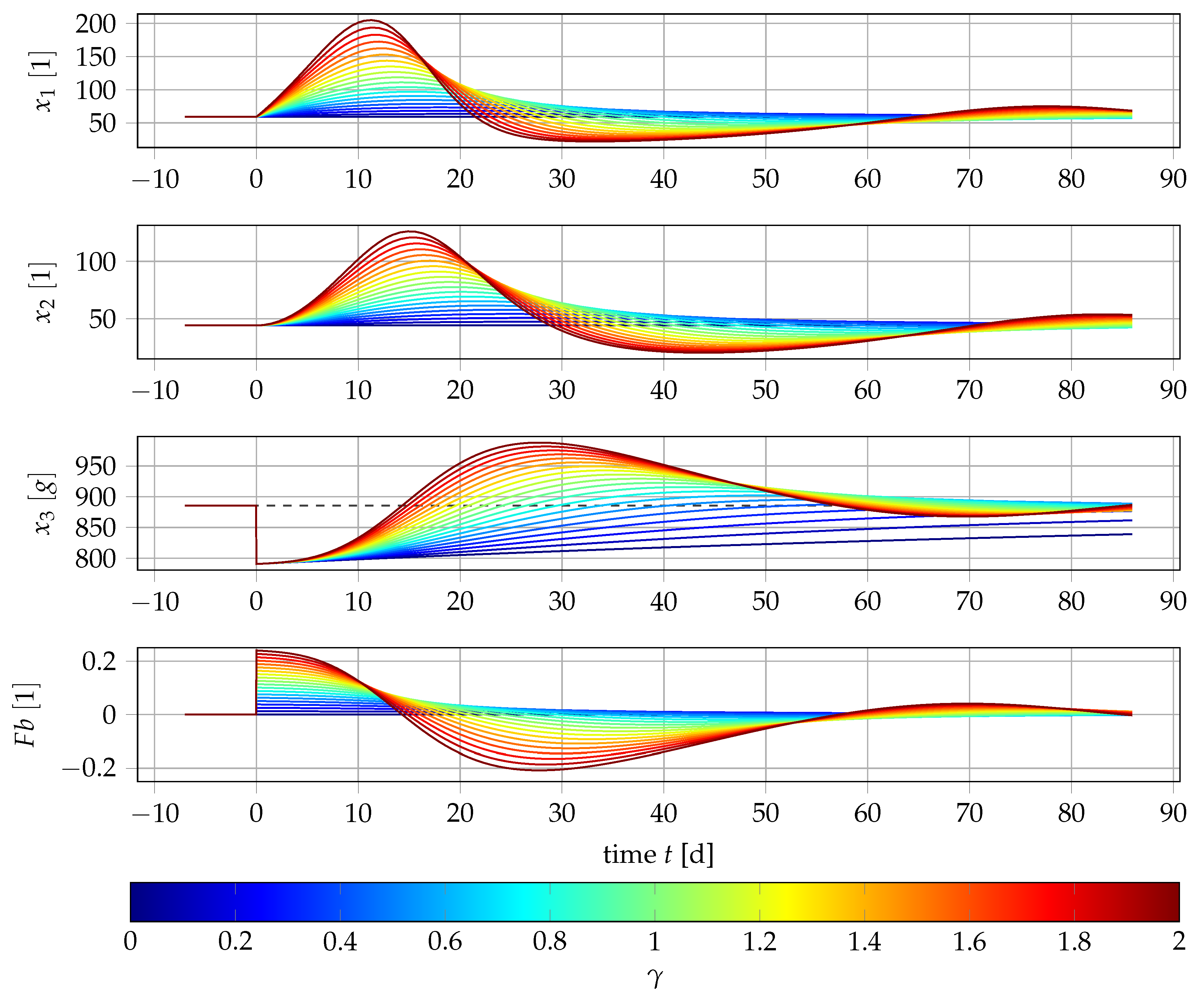
2.4. Sensitivity Analysis
2.5. Local Error Analysis of the System near the Steady State
3. Methods
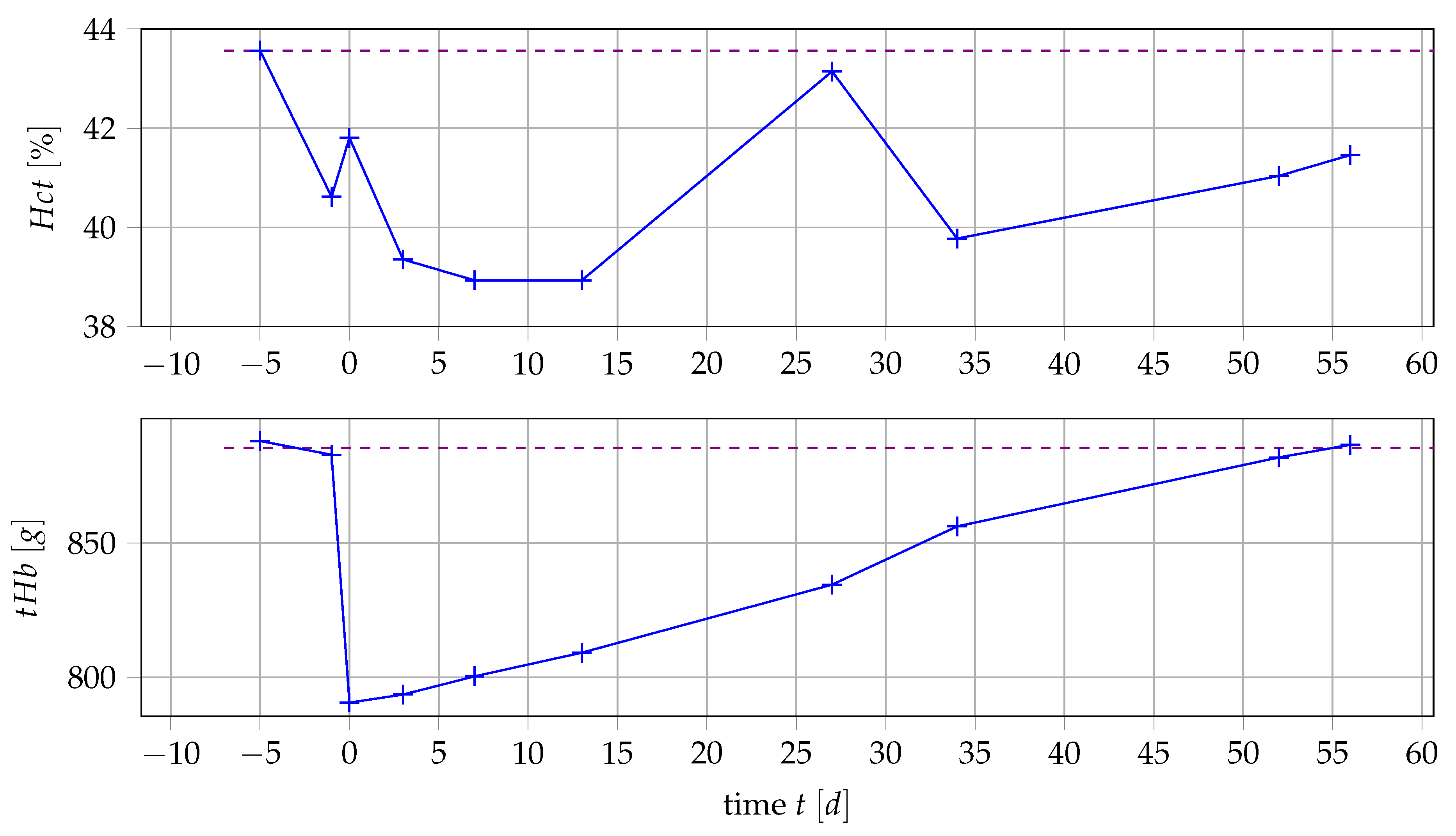
3.1. Data
3.2. Relationship of Values and Number of Erythrocytes
3.3. Calculation of Value and Blood Loss
3.4. Parameter Estimation
- are the number of available measurements of the subjects ,
- is the measurement value of at time ,
- is the according model response at time ,
- is the standard deviation of the measurement at time ,
- p is the chosen parameter vector,
- F contains the right hand sides of the model Equation (5),
- fixed start values, and
- is a term that can be used to incorporate a priori information, in our setting chosen as 0
4. Numerical Results
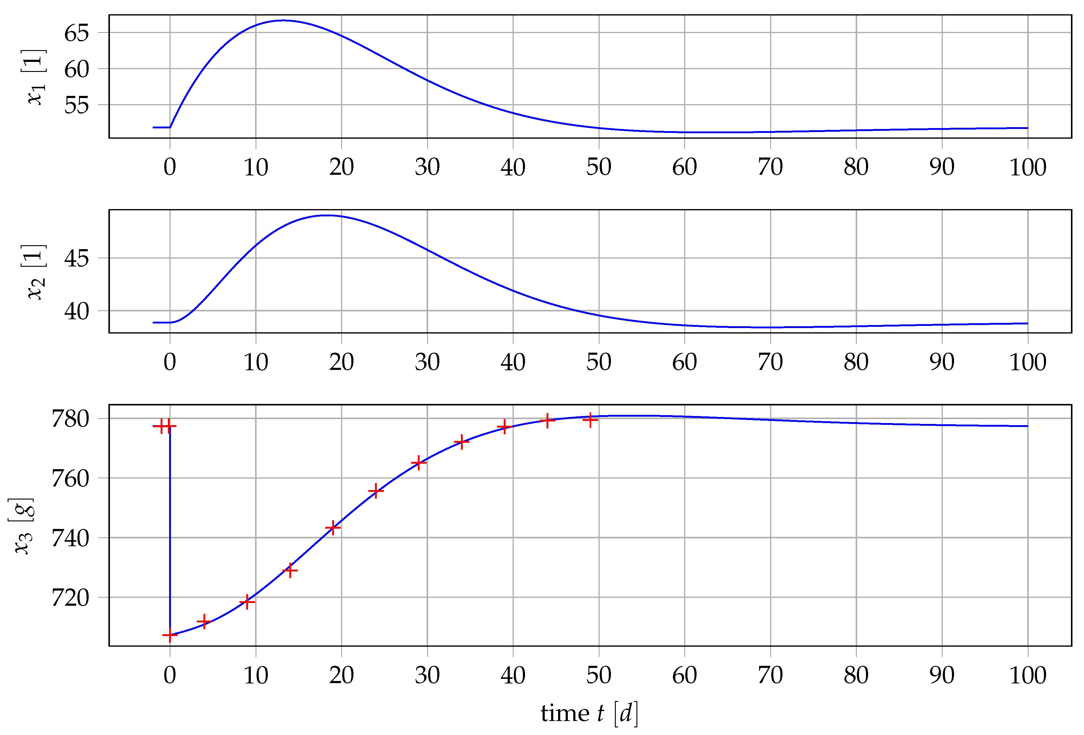
4.1. Results for Generic Subject Data from Literature
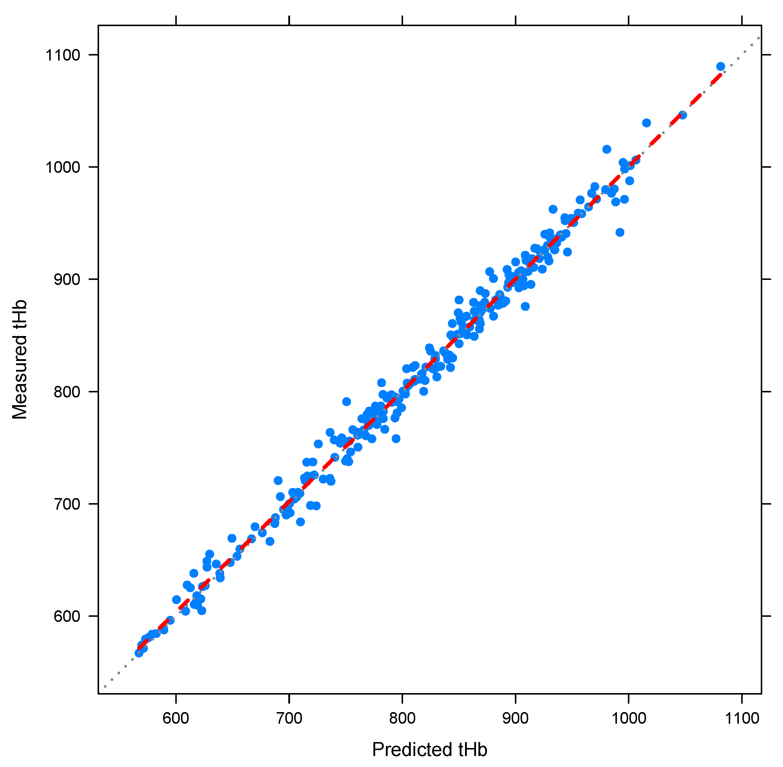
4.2. Nonlinear Mixed-Effects Estimation for and
4.3. Point Estimation Results for and
4.4. Results if Is a Free Parameter
5. Outlook: Polycythemia Vera
5.1. Obtaining Data for PV Patients
5.2. Extending the Mathematical Model
5.3. Formulating and Solving Optimization Problems
6. Conclusions
Author Contributions
Funding
Acknowledgments
Conflicts of Interest
Abbreviations
| ALL | Acute Lymphoblastic Leukemia |
| AML | Acute Myeloid Leukemia |
| BFU-E | Blast Forming Unit-Hematopoietic |
| CFU-E | Colony Forming Unit-Hematopoietic |
| DDE | Delay Differential Equation |
| EPO | Erythropoietin |
| Hct | Hematocrit |
| IVP | Initial Value Problem |
| MCH | Mean Corpuscular Hemoglobin |
| ODE | Ordinary Differential Equation |
| PDE | Partial Differential Equation |
| PK/PD | Pharmacokinetic/Pharmacodynamic |
| PV | Polycythemia vera |
| RBC | Red Blood Cell |
| SD | Standard Deviation |
| tHb | Total hemoglobin |
| WBC | White Blood Cell |
| %SD | Percentage Standard Deviation |
Appendix A. Computational Details
Appendix A.1. How to Calculate P
Appendix A.2. Analysis of the Local Error at the Steady State


Appendix B. Detailed Results

| Subject ID | SD() [%] | SD() [%]) | |||
|---|---|---|---|---|---|
| 01 | 0.769 | 13.3 | 1.65 | 26.2 | 0.961 |
| 02 | 0.388 | 12 | 0.867 | 24.4 | 0.996 |
| 03 | 0.51 | 15.3 | 1.617 | 28.7 | 0.915 |
| 04 | 0.323 | 12.4 | 0.424 | 24.2 | 0.801 |
| 05 | 0.061 | 341.6 | 1.381 | 84.9 | 0.61 |
| 06 | 0.59 | 20.6 | 2.615 | 33.4 | 0.915 |
| 07 | 0.262 | 67.9 | 1.518 | 69.7 | 0.887 |
| 08 | 0.324 | 53.3 | 2.676 | 49.1 | 0.911 |
| 09 | 0.356 | 16.6 | 0.891 | 29.7 | 0.806 |
| 10 | 0.089 | 242.2 | 2.557 | 61 | 0.947 |
| 11 | 0.243 | 20.7 | 0.925 | 29 | 0.897 |
| 12 | 1.003 | 12.5 | 1.409 | 20.1 | 0.959 |
| 13 | 0.057 | 178.1 | 0.879 | 67.8 | 0.895 |
| 14 | 0.762 | 42.7 | 0.46 | 53.6 | 0.507 |
| 15 | 0.344 | 33.1 | 2.132 | 40.9 | 0.863 |
| 16 | 0.141 | 257.3 | 1.661 | 116.9 | 0.344 |
| 17 | 0.47 | 66.2 | 0.544 | 69.1 | 0.842 |
| 18 | 0.525 | 8.8 | 0.631 | 20.1 | 0.871 |
| 19 | 0.423 | 44.7 | 1.525 | 56.2 | 0.624 |
| 20 | 0.661 | 31.1 | 2.798 | 47.9 | 0.812 |
| 21 | 0.686 | 20.9 | 1.943 | 36.7 | 0.92 |
| 23 | 0.613 | 36.1 | 3.142 | 49 | 0.897 |
| 24 | 0.421 | 26.9 | 1.528 | 42.1 | 0.905 |
| 25 | 0.863 | 15.9 | 2.078 | 24.7 | 0.868 |
| 26 | 0.414 | 16.3 | 1.172 | 29.8 | 0.703 |
| 27 | 0.635 | 8.2 | 0.836 | 16.8 | 0.866 |
| 28 | 0.952 | 15.8 | 1.596 | 26.1 | 0.992 |
| 29 | 0.805 | 22.2 | 1.486 | 39.9 | 0.925 |
| Subject ID | Base | SD(Base) [%] | SD() [%] | ||
|---|---|---|---|---|---|
| 01 | 861.014 | 1.3 | 1.685 | 21.2 | 0.963 |
| 02 | 882.041 | 1.2 | 0.838 | 17.6 | 0.996 |
| 03 | 856.779 | 0.7 | 1.296 | 14.4 | 0.907 |
| 04 | 881.885 | 3.3 | 0.431 | 22.9 | 0.806 |
| 05 | 930.774 | 1.2 | 1.306 | 44.4 | 0.595 |
| 06 | 986.155 | 0.5 | 1.985 | 12.2 | 0.899 |
| 07 | 954.28 | 2.1 | 0.968 | 43 | 0.78 |
| 08 | 692.458 | 0.8 | 1.286 | 14.1 | 0.861 |
| 09 | 956.621 | 1.4 | 0.787 | 21.2 | 0.803 |
| 10 | 815.247 | 0.9 | 1.345 | 19.1 | 0.897 |
| 11 | 980.574 | 1.1 | 0.851 | 17.7 | 0.902 |
| 12 | 936.771 | 0.7 | 1.665 | 13.9 | 0.949 |
| 13 | 611.74 | 2.5 | 0.64 | 45.3 | 0.876 |
| 14 | 1554.83 | 69 | 0.324 | 75.7 | 0.495 |
| 15 | 922.955 | 0.5 | 1.466 | 13.1 | 0.833 |
| 16 | 726.472 | 1.1 | 2.015 | 54 | 0.426 |
| 17 | 973.967 | 29.8 | 0.484 | 100.7 | 0.842 |
| 18 | 874.356 | 2.9 | 0.661 | 19.9 | 0.876 |
| 19 | 766.033 | 2.4 | 1.569 | 47 | 0.622 |
| 20 | 758.275 | 0.6 | 2.055 | 16 | 0.803 |
| 21 | 896.036 | 1 | 2.001 | 23.9 | 0.928 |
| 23 | 880.509 | 0.6 | 2.245 | 17.5 | 0.904 |
| 24 | 680.758 | 2.3 | 1.304 | 33.2 | 0.895 |
| 25 | 772.443 | 0.7 | 1.675 | 12.6 | 0.87 |
| 26 | 686.724 | 1.8 | 0.925 | 21.1 | 0.695 |
| 27 | 947.998 | 1.5 | 0.859 | 16.1 | 0.884 |
| 28 | 872.556 | 1.1 | 1.684 | 21.1 | 0.991 |
| 29 | 812.567 | 3 | 1.478 | 41.6 | 0.925 |
References
- Jandl, J.H. Blood, 1st ed.; Little Brown: Boston, MA, USA, 1987. [Google Scholar]
- Lichtman, M.A.; Beutler, E.; Kipps, T.J.; Seligsohn, U.; Kaushansky, K.; Prchal, J.T. Williams Hematology; McGraw-Hill: New York, NY, USA, 2006. [Google Scholar]
- Mackey, M.C.; Glass, L. Oscillation and chaos in physiological control systems. Science 1977, 197, 287–289. [Google Scholar] [CrossRef] [PubMed]
- Loeffler, M.; Pantel, K.; Wulff, H.; Wichmann, H. A mathematical model of erythropoiesis in mice and rats Part 1: Structure of the model. Cell Prolif. 1989, 22, 13–30. [Google Scholar] [CrossRef]
- Bélair, J.; Mackey, M.C.; Mahaffy, J.M. Age-structured and two-delay models for erythropoiesis. Math. Biosci. 1995, 128, 317–346. [Google Scholar] [CrossRef]
- Mahaffy, J.M.; Polk, S.W.; Roeder, R.K. An Age-Structured Model for Erythropoiesis Following a Phlebotomy; Department of Mathematical Sciences, San Diego State University: San Diego, CA, USA, 1999. [Google Scholar]
- Ackleh, A.; Thibodeaux, J. Parameter estimation in a structured erythropoiesis model. Math. Biosci. Eng. 2008, 5, 601–616. [Google Scholar] [CrossRef] [PubMed] [Green Version]
- Fuertinger, D.H.; Kappel, F.; Thijssen, S.; Levin, N.W.; Kotanko, P. A model of erythropoiesis in adults with sufficient iron availability. J. Math. Biol. 2013, 66, 1209–1240. [Google Scholar] [CrossRef] [PubMed]
- Edelstein-Keshet, L. Mathematical Models in Biology; Society for Industrial and Applied Mathematics: Philadelphia, PA, USA, 2005; Volume 46, pp. 27–33. [Google Scholar]
- Fonseca, L.L.; Voit, E.O. Comparison of mathematical frameworks for modeling erythropoiesis in the context of malaria infection. Math. Biosci. 2015, 270, 224–236. [Google Scholar] [CrossRef] [PubMed] [Green Version]
- Friberg, L.E.; Henningsson, A.; Maas, H.; Nguyen, L.; Karlsson, M.O. Model of chemotherapy-induced myelosuppression with parameter consistency across drugs. J. Clin. Oncol. 2002, 20, 4713–4721. [Google Scholar] [CrossRef] [PubMed]
- Rinke, K.; Jost, F.; Findeisen, R.; Fischer, T.; Bartsch, R.; Schalk, E.; Sager, S. Parameter estimation for leukocyte dynamics after chemotherapy. IFAC-PapersOnLine 2016, 49, 44–49. [Google Scholar] [CrossRef]
- Jost, F.; Rinke, K.; Fischer, T.; Schalk, E.; Sager, S. Optimum experimental design for patient specific mathematical leukopenia models. IFAC-PapersOnLine 2016, 49, 344–349. [Google Scholar] [CrossRef]
- Crauste, F.; Demin, I.; Gandrillon, O.; Volpert, V. Mathematical study of feedback control roles and relevance in stress erythropoiesis. J. Theor. Biol. 2010, 263, 303–316. [Google Scholar] [CrossRef] [PubMed]
- Mackey, M.C. A unified hypothesis for the origin of aplastic anemia and periodic haematopoiesis. Blood 1978, 51, 941–956. [Google Scholar] [PubMed]
- Noble, S.L.; Sherer, E.; Hannemann, R.E.; Ramkrishna, D.; Vik, T.; Rundell, A.E. Using adaptive model predictive control to customize maintenance therapy chemotherapeutic dosing for childhood acute lymphoblastic leukemia. J. Theor. Biol. 2010, 264, 990–1002. [Google Scholar] [CrossRef] [PubMed]
- Pottgiesser, T.; Specker, W.; Umhau, M.; Dickhuth, H.H.; Roecker, K.; Schumacher, Y.O. Recovery of hemoglobin mass after blood donation. Transfusion 2008, 48, 1390–1397. [Google Scholar] [CrossRef] [PubMed]
- Ertl, A.C.; Diedrich, A.; Raj, S.R. Techniques Used for the Determination of Blood Volume. Am. J. Med. Sci. 2007, 334, 32–36. [Google Scholar] [CrossRef] [PubMed]
- Otto, J.M.; Plumb, J.O.; Clissold, E.; Kumar, S.B.; Wakeham, D.J.; Schmidt, W.; Grocott, M.P.; Richards, T.; Montgomery, H.E. Hemoglobin concentration, total hemoglobin mass and plasma volume in patients: implications for anemia. Haematologica 2017, 102, 1477–1485. [Google Scholar] [CrossRef] [PubMed] [Green Version]
- Passamonti, F.; Malabarba, L.; Orlandi, E.; Baratè, C.; Canevari, A.; Brusamolino, E.; Bonfichi, M.; Arcaini, L.; Caberlon, S.; Pascutto, C.; et al. Polycythemia vera in young patients: a study on the long-term risk of thrombosis, myelofibrosis and leukemia. Haematologica 2003, 88, 13–18. [Google Scholar] [PubMed]
- Siegel, F.P.; Tauscher, J.; Petrides, P.E. Aquagenic pruritus in polycythemia vera. Am. J. Hematol. 2013, 88, 665–669. [Google Scholar] [CrossRef] [PubMed]
- Marchioli, R. Vascular and Neoplastic Risk in a Large Cohort of Patients With Polycythemia Vera. J. Clin. Oncol. 2005, 23, 2224–2232. [Google Scholar] [CrossRef] [PubMed]
- Ziegler, A.K.; Grand, J.; Stangerup, I.; Nielsen, H.J.; Dela, F.; Magnussen, K.; Helge, J.W. Time course for the recovery of physical performance, blood hemoglobin, and ferritin content after blood donation. Transfusion 2015, 55, 898–905. [Google Scholar] [CrossRef] [PubMed]
- Wide, L.; Bengtsson, C.; Birgegárrd, G. Circadian rhythm of erythropoietin in human serum. Br. J. Haematol. 1989, 72, 85–90. [Google Scholar] [CrossRef] [PubMed]
- Marciniak-Czochra, A.; Stiehl, T.; Ho, A.D.; Jäger, W.; Wagner, W. Modeling of asymmetric cell division in hematopoietic stem cells—Regulation of self-renewal is essential for efficient repopulation. Stem Cells Dev. 2009, 18, 377–386. [Google Scholar] [CrossRef] [PubMed]
- Spiegel, M.R. Mathematical Handbook of Formulas and Tables; McGraw-Hill: New York, NY, USA, 1968. [Google Scholar]
- Schmidt, W.; Prommer, N. The optimised CO-rebreathing method: A new tool to determine total haemoglobin mass routinely. Eur. J. Appl. Physiol. 2005, 95, 486–495. [Google Scholar] [CrossRef] [PubMed]
- Masoud, M.; Sarig, G.; Brenner, B.; Jacob, G. Orthostatic Hypercoagulability. Hypertension 2008, 51, 1545–1551. [Google Scholar] [CrossRef] [PubMed] [Green Version]
- Wadsworth, G.R. Recovery from acute haemorrhage in normal men and women. J. Physiol. 1955, 129, 583–593. [Google Scholar] [CrossRef] [PubMed] [Green Version]
- Bock, H.G.; Körkel, S.; Schlöder, J.P. Parameter Estimation and Optimum Experimental Design for Differential Equation Models. In Model Based Parameter Estimation: Theory and Applications; Bock, H.G., Carraro, T., Jäger, W., Körkel, S., Rannacher, R., Schlöder, J.P., Eds.; Springer: Heidelberg, Germany, 2013; pp. 1–30. [Google Scholar]
- Convertino, V.A. Blood Volume Response to Physical Activity and Inactivity. Am. J. Med. Sci. 2007, 334, 72–79. [Google Scholar] [CrossRef] [PubMed]
- Eaves, C.J.; Eaves, A.C. Erythropoietin (Ep) dose-response curves for three classes of erythroid progenitors in normal human marrow and in patients with polycythemia vera. Blood 1978, 52, 1196–1210. [Google Scholar] [PubMed]


| State | Explanation | Value | Unit |
|---|---|---|---|
| Erythroid progenitor cells highly proliferating with respect to erythropoietin (EPO) | 59.03 | [1] | |
| Erythroid progenitor cells not proliferating with respect to EPO | 44.27 | [1] | |
| Mature erythrocytes and blood reticulocytes | 885.42 | [g] | |
| Parameter | |||
| Mean erythrocyte count in steady state | 885.42 | [g] | |
| Committed stem cells transitioning into | 7.3785 | [] | |
| Transition rate from to | 0.125 | [] | |
| Transition rate from to | 0.1667 | [] | |
| * | Apoptosis rate of | −0.00833 | [] |
| ** | Amplifying factor for individual blood regeneration, global factor independent of fraction of blood loss | 1.0 | [1] |
| ** | Amplifying factor for individual blood regeneration, depending on fractional blood loss | 0.3 | [] |
| Feedback function depending on fractional blood loss | 0.0 | [1] |
© 2018 by the authors. Licensee MDPI, Basel, Switzerland. This article is an open access article distributed under the terms and conditions of the Creative Commons Attribution (CC BY) license (http://creativecommons.org/licenses/by/4.0/).
Share and Cite
Tetschke, M.; Lilienthal, P.; Pottgiesser, T.; Fischer, T.; Schalk, E.; Sager, S. Mathematical Modeling of RBC Count Dynamics after Blood Loss. Processes 2018, 6, 157. https://doi.org/10.3390/pr6090157
Tetschke M, Lilienthal P, Pottgiesser T, Fischer T, Schalk E, Sager S. Mathematical Modeling of RBC Count Dynamics after Blood Loss. Processes. 2018; 6(9):157. https://doi.org/10.3390/pr6090157
Chicago/Turabian StyleTetschke, Manuel, Patrick Lilienthal, Torben Pottgiesser, Thomas Fischer, Enrico Schalk, and Sebastian Sager. 2018. "Mathematical Modeling of RBC Count Dynamics after Blood Loss" Processes 6, no. 9: 157. https://doi.org/10.3390/pr6090157
APA StyleTetschke, M., Lilienthal, P., Pottgiesser, T., Fischer, T., Schalk, E., & Sager, S. (2018). Mathematical Modeling of RBC Count Dynamics after Blood Loss. Processes, 6(9), 157. https://doi.org/10.3390/pr6090157