Energy and Exergy Analysis of the S-CO₂ Brayton Cycle Coupled with Bottoming Cycles

Abstract

Supercritical carbon dioxide (S-CO₂) Brayton cycles (BC) are soon to be a competitive and environment friendly power generation technology. Progressive technological developments in turbo-machineries and heat exchangers have boosted the idea of using S-CO₂ in a closed-loop BC. This paper describes and discusses energy and exergy analysis of S-CO₂ BC in cascade arrangement with a secondary cycle using CO₂, R134a, ammonia, or argon as working fluids. Pressure drop in the cycle is considered, and its effect on the overall performance is investigated. No specific heat source is considered, thus any heat source capable of providing temperature in the range from 500 °C to 850 °C can be utilized, such as solar energy, gas turbine exhaust, nuclear waste heat, etc. The commercial software ‘Aspen HYSYS version 9’ (Aspen Technology, Inc., Bedford, MA, USA) is used for simulations. Comparisons with the literature and simulation results are discussed first for the standalone S-CO₂ BC. Energy analysis is done for the combined cycle to inspect the parameters affecting the cycle performance. The second law efficiency is calculated, and exergy losses incurred in different components of the cycle are discussed.

1. Introduction

Gas turbines (GT) are inevitable in modern power generation. The simple GT cycle has poor efficiency due to the elevated temperature of flue gases. To improve the fuel efficiency, the simple GT cycle is generally coupled with a bottoming cycle in stationary variants of GT, like the conventional steam Rankine cycles (RC) and the organic Rankine cycles (ORC) [1,2]. The rapid development of industries around the world has resulted in an increasing demand of energy. The shortage of fossil energy prompts people to investigate more efficient gas turbine combined cycles to meet the energy requirements. Exploiting low-grade waste heat for energy production is an attractive option for its potential to reduce fossil fuel consumption. When exploiting medium-temperature heat sources, supercritical carbon dioxide (S-CO₂) is advantageous because of its high efficiency, compactness, and cost [3,4]. Many pilot-scale facilities have been developed in the last few years to investigate the performance of S-CO₂ BC (Brayton cycles) [5,6,7,8]. When utilizing low-grade waste heat, the traditional steam Rankine cycle does not give satisfying results because of poor thermal efficiency, thus the organic Rankine cycles and transcritical CO₂ (t-CO₂) cycles are proposed [9,10,11,12].

The supercritical state of CO₂ as working fluid in BC has various advantages. Its critical temperature is low (31.1 °C), which allows to use the natural resources of water as a cooling medium in the condenser. The density of CO₂ close to the critical point is similar to that of a liquid and allows to decrease the compressor work significantly. CO₂ in its supercritical state is almost twice as dense as steam. This results in very high power density, which allows to drastically reduce the compressor and turbine size. S-CO₂ BC is compatible with a variety of renewable heat sources, thus it has little impact on the environment with low to no ozone depletion potential. Atif and Al-Sulaiman [13,14] presented the energy and exergy analysis of solar-driven S-CO₂ and its applicability in desert climates, like in Saudi Arabia. Kun Wang [15] studied S-CO₂ recompression Brayton cycle (RBC) with molten salt solar power. He developed a model to investigate the effects of salt temperature, compressor inlet conditions, and heliostat orientation on the overall cycle efficiency. Hou et al. recently examined S-CO₂ recompression and regenerative cycle utilizing waste heat energy from a marine gas turbine [16]. They found a 13% overall thermal efficiency improvement with the combined cycle. Wang et al. [17] worked on the cascaded S-CO₂ cycle integrating solar and biomass.

S-CO₂ working with a medium-temperature source may be coupled with a bottoming cycle, which utilizes low-grade waste heat of the primary cycle and rejects in a low-temperature sink [18]. Wang et al. investigated the t-CO₂ cycle to exploit low-grade geothermal sources for electricity production [19]. They used liquefied natural gas (LNG) as a low-temperature heat sink to allow low back pressure of the CO₂ turbine, thus greatly improving the overall performance of the cycle. Ahmadi et al. established a similar energy conversion system and showed a significant contribution of t-CO₂ in geothermal energy utilization [20]. Amini et al. exploited the low-grade energy of exhaust gas (150 °C) from a combined cycle power plant to run the t-CO₂ cycle. The results indicated a significant improvement of power output and efficiency [21]. Walnum et al. concluded that a dual-stage t-CO₂ system performs better in offshore gas turbines [22]. Wu et al. reported that t-CO₂ has the potential to recover medium-grade heat and suggested that more stages should be designed with the increase of waste heat temperature [23].

Much research has been dedicated to the thermodynamic analysis of supercritical CO₂ BC utilizing medium-temperature heat either from renewable sources or from gas turbine exhausts. Some studies have been carried out on the utilization of low-grade heat of S-CO₂ BC using the t-CO₂ cycle as a bottoming cycle. However, little attention has been paid to the effect of pressure drop in the system. S-CO₂ RBC is efficient for medium to high-temperature sources, which offer low-grade heat energy (with a temperature of about 100 °C to 120 °C). In the present study, a simulation investigation is done to seek parameters that could possibly improve the overall cycle’s efficiency. We consider various working fluids, including CO₂, in the bottoming cycle, utilizing low-grade heat energy from S-CO₂ RBC as a primary cycle. Implementing the bottoming cycle with a low-temperature heat source requires to maintain the sink medium at a very low temperature. Liquefied natural gas (LNG) contains a large amount of cold energy, naturally making it a suitable candidate for providing a low-temperature sink medium [24,25,26,27].

The selection of appropriate working fluids depends on many factors and properties, such as critical temperature and pressure, chemical stability at the operating temperature, environment friendliness, economic convenience, and allows a high utilization of the energy available from the heat source. Considering the maximum temperature available for the bottoming cycle, i.e., about 120 °C, CO₂, R134a, ammonia, and argon were chosen as potential candidates for the present study. R134a has zero ozone depletion potential (ODP). It has already been used commercially, and the necessary equipment, such as heat exchangers and turbo-machines, is readily available. It has a critical temperature of 101.1 °C, allowing it to be used in the temperature range of interest. Ammonia, despite being toxic and flammable, is one of the most environment friendly working fluid with zero ODP and zero global warming potential (GWP). It is being used in industries and is considered a highly efficient refrigerant. It has a critical temperature of 132.4 °C, which allows to adopt it as a working fluid for the available heat source. The bottoming cycle utilizing CO₂, R134a, and ammonia is similar to the Rankine cycle, thus it requires a pump to maintain the cycle pressure ratio. Moreover, the performance of argon was also studied in the bottoming cycle, which is similar to the Brayton cycle. Argon was selected because of its high density, which allows to employ compact turbo-machines with fewer stages.

The first part of the article discusses the configuration of the simulation environment, the adjustment of the operational parameters, and the mathematical model for energy and exergy analysis. The model is validated by comparing the results for the supercritical CO₂ recompression Brayton cycle with previous findings. The second part of the paper presents the results of the energy analysis. The potential improvements in the overall efficiency with the bottoming cycle utilizing different working fluids (CO₂, argon, ammonia, R134a) are outlined. The last part of the paper addresses the results of the exergy analysis. The exergy loss in various components of the cycle is calculated. This analysis could help in selecting the working fluids suitable for the bottoming cycle.

2. System Configuration, Modeling, and Simulation Environment

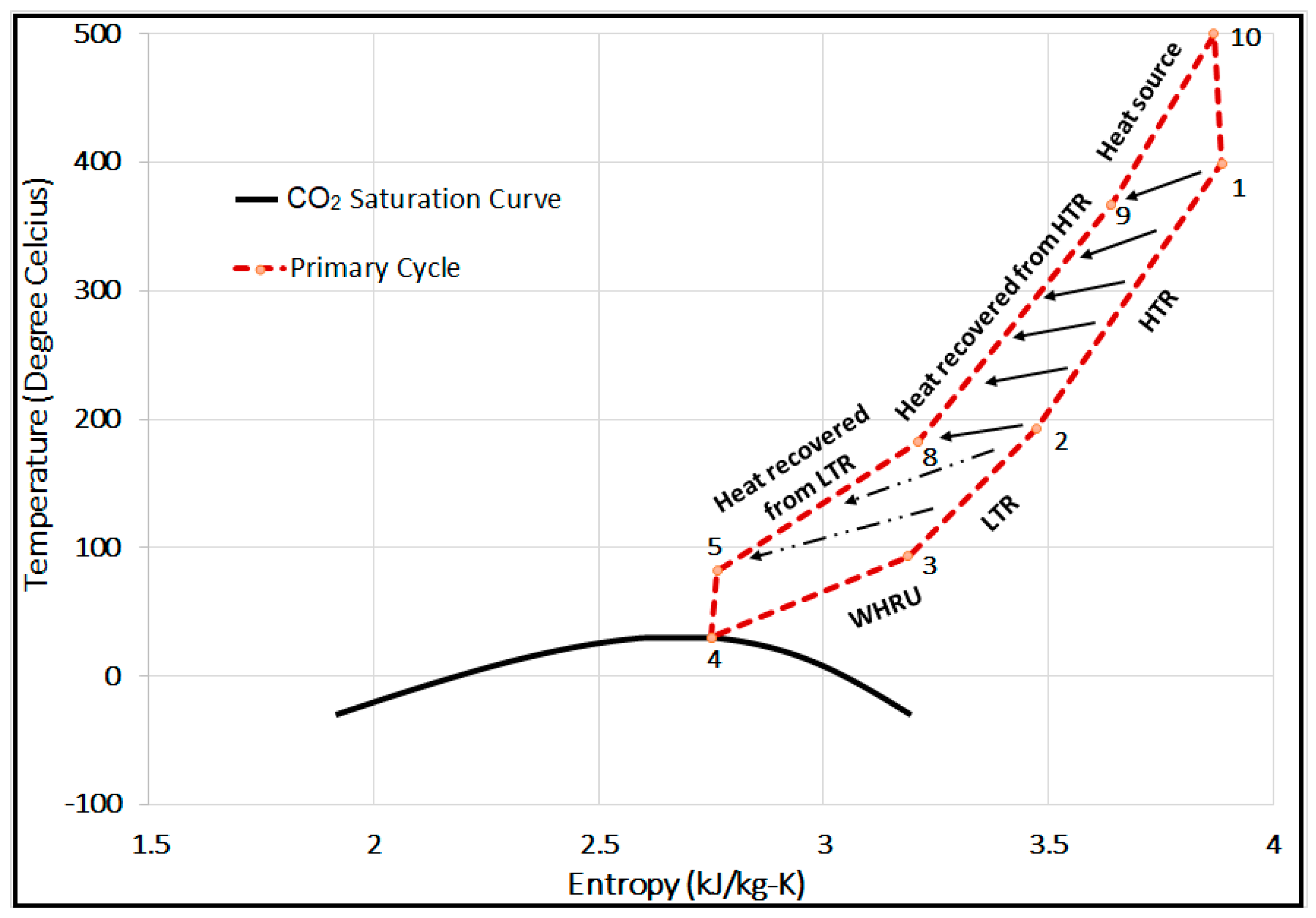
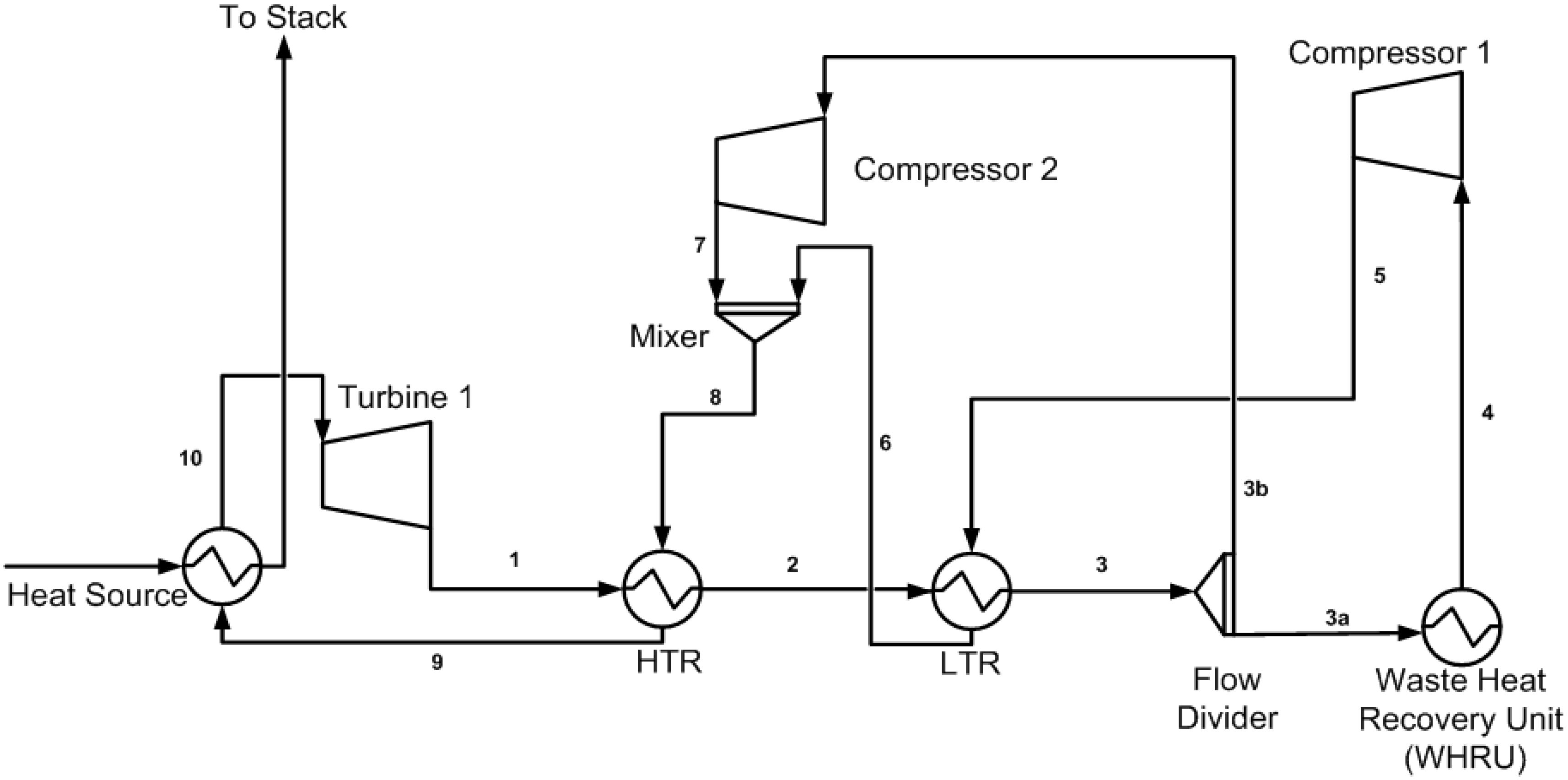
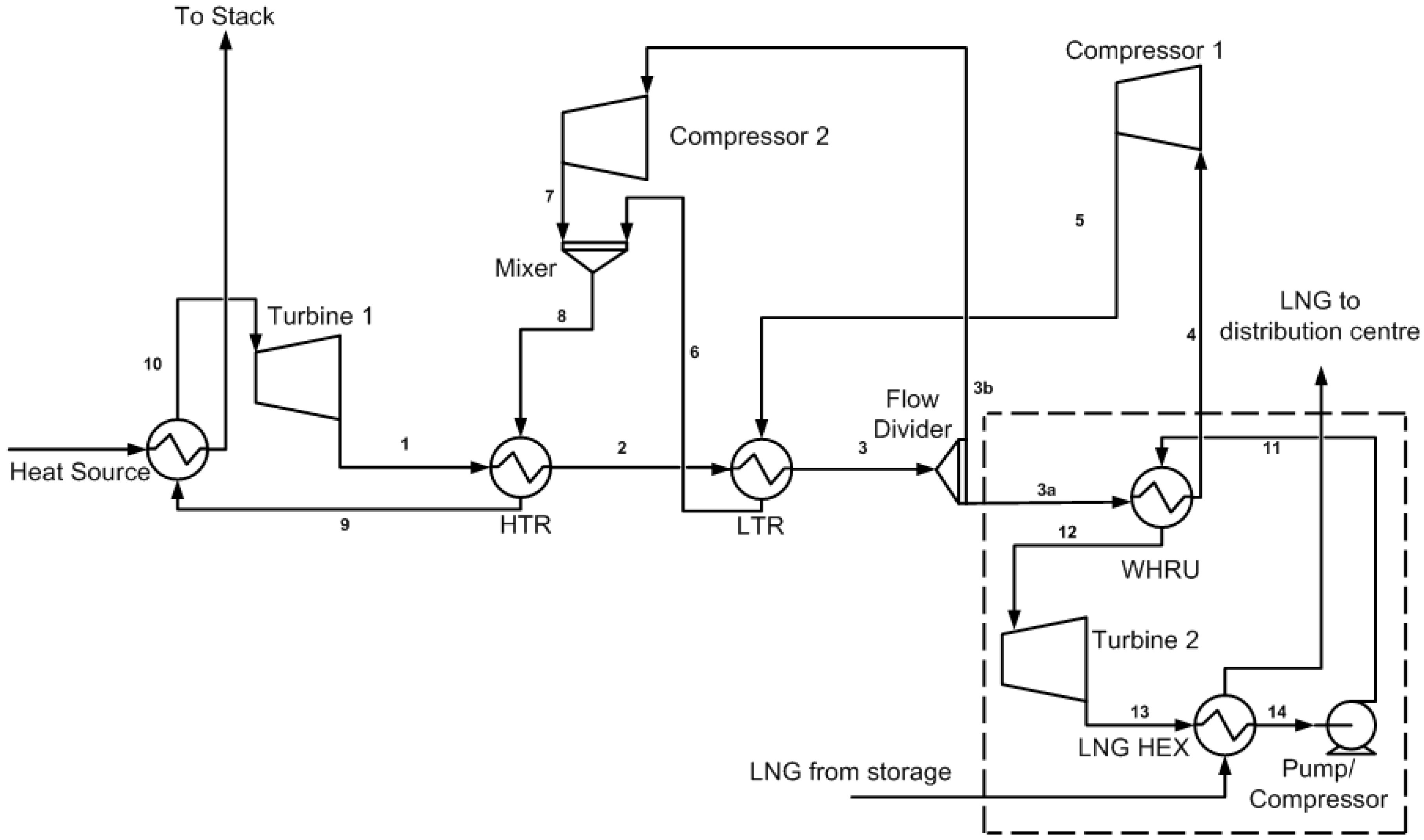
2.1. Primary Cycle (Base Model) Layout for the S-CO₂ Cycle

The base model is a recompression Brayton cycle (RBC) with partial condensation. This layout was originally proposed by Feher [28] and Angelio [29], then refined by Dostal [30]. They observed that large internal irreversibility losses occurred in the case of a fully condensing cycle due to heat recuperation between the low heat capacity turbine exhaust and the high heat capacity flow from the pump. Thus, partial condensation was proposed to reduce these losses. This was done by splitting the stream from the turbine exhaust. The term flow ratio ‘x’ is generally used to indicate the magnitude of the divided mass flow rate. The layout of the cycle is shown in Figure 1. The stream leaving the low-temperature recuperator (LTR) is divided into two streams. The first stream (State 3a) goes to Compressor 1 and the second stream (State 3b) goes to Compressor 2, which is a recompressor operating at the exit temperature and pressure of the LTR. The stream leaving Compressor 1 (State 5) passes through the LTR where it receives energy from the hotter stream (State 2) and is then mixed with the stream (State 7) leaving Compressor 2. The mixed stream (State 8) is further heated in the high-temperature recuperator (HTR) before it receives heat from the heat source. Finally, it expands in Turbine 1. Part of the work produced in Turbine 1 is used to drive Compressor 1 and Compressor 2.

2.2. Cycle Cascade of the S-CO₂ Combined Cycle

Figure 2 illustrates the schematic diagram of the combined cycle based on the cold energy utilization of LNG. The secondary cycle runs on the energy recovered from the primary cycle in the waste heat recovery unit (WHRU). The working fluid in the secondary cycle receives heat energy from the WHRU and then expands in Turbine 2. After expansion, it rejects heat to the low-temperature sink, which is a liquefied natural gas heat exchanger (LNG HEX). The stream then goes to a pump or a compressor, depending on the state of the working fluid. Part of the work produced by Turbine 2 is consumed to drive the pump or compressor of the secondary cycle.

3. Mathematical Model

3.1. Energy Analysis—Governing Equations

The primary cycle efficiency (η_pc) and combined cycle efficiency (η_cc) are calculated by:

η_pc = (W_T1 − W_C1 − W_C2)/Q_IN

(1)

η_cc = (W_T1 + W_T2 − W_C1 − W_C2 − W_P)/Q_IN

(2)

W_T1 = m_PC (h₁₀ − h₁)

(3)

W_T2 = m_SC (h₁₂ − h₁₃)

(4)

W_C1 = m_C1 (h₄ − h₅)

(5)

W_C2 = m_C2 (h₈ − h₃)

(6)

W_Pump = m_SC (h₁₁ − h₁₄)

(7)

Q_IN = m_PC (h₁₀ − h₉)

(8)

where m_PC, m_SC, m_C1, m_C2 are the mass flow rates through the primary cycle, secondary cycle, Compressor 1, and Compressor 2, respectively. ‘Q_IN’ represents the total heat input per unit time given to the cycle; ‘h’ represents enthalpy, and the subscript numbers are associated with the state points shown in Figure 2. The ratio of total mass flow rate in the primary cycle returning to Compressor 1 is defined by the variable ‘x’ and is equal to:

x = m_C1/m_PC

(9)

The heat exchange between primary and secondary cycle via WHRU is governed by the following energy balance:

m_C1 (h₄ − h₃) = m_SC (h₁₂ − h₁₁)

(10)

A minimum temperature approach is enforced and set to 10 °C. Heat transfer in the HTR and LTR obeys the following governing equations, which are also set to exchange heat using a minimum temperature approach of 10 °C

(h₁ − h₂) = (h₉ − h₈)

(11)

(h₂ − h₃) = x (h₈ − h₅)

(12)

3.2. Exergy Analysis—Governing Equations

The exergy destroyed (Χ_destroyed) in each of the components of the cycle is calculated according to the following equations. The kinetic and potential energy change is neglected.

Χ_{destroyed, C1} = m_C1 T_surr (s₅ − s₄)

(13)

Χ_{destroyed, C2} = m_C2 T_surr (s₇ − s_3b)

(14)

Χ_{destroyed, T1} = m_PC T_surr (s₁ − s₁₀)

(15)

Χ_{destroyed, T2} = m_SC T_surr (s₁₃ − s₁₂)

(16)

Χ_{destroyed, HTR} = m_PC T_surr [(s₂ − s₁) + (s₉ − s₈)]

(17)

Χ_{destroyed, LTR} = m_PC T_surr [x(s₆ − s₅) + (s₃ − s₂)]

(18)

Χ_{destroyed, WHRU} = T_surr [m_SC (s₁₂ − s₁₁) + m_PC x(s₄ − s_3a)]

(19)

Χ_{destroyed, LNG HEX} = T_surr [m_SC (s₁₄ − s₁₃) + m_LNG (Δs_LNG)]

(20)

Χ_{destroyed, Pump} = m_SC T_surr (s₁₁ − s₁₄)

(21)

where T_surr is the surrounding temperature, and ‘s’ represents entropy.

The second law efficiency of the cycle is calculated as

η_II = (W_T1 + W_T2 − W_C1 − W_C2 − W_P)/(ψ_T1 + ψ_T2 − ψ_C1 − ψ_C2 − ψ_Pump)

(22)

where ψ represents reversible work and is defined as

ψ_T1 = m_PC [(h₁₀ − h₁) − T_surr (s₁₀ − s₁)]

(23)

ψ_T2 = m_SC [(h₁₂ − h₁₃) − T_surr (s₁₂ − s₁₃)]

(24)

ψ_C1 = m_PC (x) [(h₅ − h₄) − T_surr (s₅ − s₄)]

(25)

ψ_C2 = m_PC (1 − x) [(h₇ − h_3b) − T_surr (s₇ − s_3b)]

(26)

ψ_Pump = m_SC [(h₁₁ − h₁₄) − T_surr (s₁₁ − s₁₄)]

(27)

4. Simulation Environment and Procedure

The commercial software Aspen HYSYS V9 (Aspen Technology, Inc., Bedford, MA, USA)was used to simulate the cycle. The Peng-Robinson model was considered for state properties calculation. The analysis was done with the following restrictions imposed:

• The cycle operates under steady-state conditions.
• Surrounding temperature is 25 °C.
• Primary cycle mass flow rate is 100 kg/s.
• LNG in the storage tank is maintained at −162 °C.
• Energy losses in the pipelines are neglected.
• Compression and expansion processes are adiabatic.
• Compressor and turbine adiabatic efficiencies are 85% and 90%, respectively.
• Adiabatic efficiency of a centrifugal pump in the secondary cycle is 80%.
• Minimum temperature approach is set to 10 degrees in HTR, LTR, WHRU, and LNG HEX.
• The state of CO₂ is kept close to the critical point at the inlet of Compressor 1, (P = 7.2 MPa and T = 30 °C).

5. Primary Cycle Parametric Adjustments

Thermodynamically, the cycle performance greatly depends on a number of parameters, such as operating pressure ratio, flow ratio, operating temperatures [28,31]. This section discusses the steps undertaken in the selection of the parameters for the cycle. Three cases were considered with different assumed pressure drop in the system. For each case, the pressure drop was considered uniform in the cycle: for example, a 2% pressure drop indicated the reduction of 2% of the inlet pressure across each heat exchanger in the cycle for both sides (hot and cold sides).

The case study was set in Aspen HYSYS to calculate the cycle efficiency for a range of flow ratios ’x’ and cycle’s pressure ratios. The results are presented as contour plots in Figure 3a–c. It is worth noting that the efficiency for each colored patch can be read with a degree of error of ±0.5. A parametric simulation study was set up to seek operational parameters (pressure ratio and flow ratio) that approximate a near-optimal operation of the cycle with respect to thermal efficiency. The best possible combination found for each case is listed in

Table 1. Optimal values of flow ratio and pressure ratio for maximum efficiency of the primary cycle.

Pressure Drop	Flow Ratio x	Compressor 1 Compression Ratio	Compressor 2 Compression Ratio	Turbine Inlet Pressure (P10) MPa
No Drop	0.66	2.40	2.40	16.60
2%	0.69	3.00	3.14	20.40
4%	0.71	3.60	3.85	24.45

.

Figure 4 represents the temperature–entropy T–S diagram of the primary cycle with a turbine inlet temperature of 500 °C. It can be observed that the LTR and HTR units recovered and recycled more than 60% of the heat.

6. Primary Cycle (Base Model) Validation and Performance

The primary cycle (S-CO₂ RBC) serves as a base model, thus it is imperative to validate the results with previously published data. Figure 5 represents the thermal efficiency plotted against the turbine inlet temperature. The simulation results are plotted along with the results published by Kun Wang [32] and Turchi et al. [33] (this study did not consider the pressure drop in the system). It is evident from the plot that the base model, developed in Aspen HYSYS V9, produced results in agreement with the previously published data. It is worth mentioning that Kim et al. [34] investigated the amount of pressure loss that could occur in a printed circuit heat exchanger (PCHE) for S-CO₂. Their study indicated a pressure loss of about 2%. Thus, if we assume a similar pressure drop, then the efficiency of 40% or above is achievable with a turbine inlet temperature of 550 °C or higher.

Figure 6 represents the back work ratio (BWR) plotted as a function of the turbine inlet temperature. The BWR is the fraction of work produced in the turbine that is consumed by the compressors in the cycle. Considering the curve for no pressure drop in Figure 6, the BWR is below 40%, which is uncommon for a standard Air Brayton cycle. The smaller BWR of the S-CO₂ RBC is due to the fact that the CO₂ is brought to the critical state before the inlet to Compressor 1, which results in reduced compressor work and improvement in the overall efficiency of the cycle.

Figure 7 represents the magnitude of efficiency improvement with respect to turbine inlet temperature. It is worth noting that the S-CO₂ recompression cycle is best suited for medium temperature range (approx. up to 850 °C). Further increase to turbine inlet temperature would increase the cost of high-temperature resistance material with no significant increase in the efficiency improvements.

7. Combined Cycle Parametric Adjustments

The secondary cycle in cascade with the primary S-CO₂ cycle was investigated using carbon dioxide, ammonia, R134a, and argon as working fluids. A minimum temperature approach of 10 degrees was used for the heat exchangers (WHRU and LNG HEX). The secondary fluid inlet temperature to the WHRU was fixed at −25 °C for all cases. The combined cycle efficiency was maximized by searching the best possible combination of primary and secondary cycle pressure ratios for all temperatures and pressure drops considered in the study. Figure 8 displays the contour plot of efficiency against a range of pressure ratios of primary and secondary cycles. It reveals that the optimum value of primary cycle pressure ratio remained at nearly the same value as when there was no bottoming cycle (see Table 1). These plots are only shown for two temperatures at different pressure drops, with CO₂ as a working fluid for the secondary or bottoming cycle; however, optimum values of primary and secondary cycle pressure ratios were obtained in the same manner for all cases discussed in this study. After expansion, the working fluid exchanged heat in the LNG HEX, where the LNG inlet temperature was fixed at −162 °C (refer to Figure 2). Afterwards, the pump or compressor raised the pressure of the working fluid according to cycle’s operating pressure ratio.

8. Combined Cycle Performance and Overall Improvement

8.1. Combined Cycle Energy Analysis

This section discusses the essential outcomes of the energy analysis for the combined cycle governed by the set of equations from 1 to 12. The maximum efficiency of the cascade S-CO₂ combined cycle was plotted against the turbine inlet temperature (T₁₀) and is shown in Figure 9. A general monotonic behavior was observed for the efficiency of the combined cycle, which increased with the turbine inlet temperature. A similar behavior of the cycle’s efficiency was observed for the standalone primary cycle (see Figure 5). The effect of pressure drop in the system was reflected in the reduction of the overall cycle’s efficiency. Ammonia and R134a were found to be the least efficient. Argon appeared to be more efficient than the other candidates. This is due to the fact that the argon cycle is similar to the Brayton cycle and incurs much smaller losses (due to no phase change). Thus, argon can expand to lower temperatures than the other candidates that run on cycles similar to the Rankine cycle.

Figure 10 illustrates the overall efficiency improvement coming from the secondary cycle with argon, CO₂, ammonia, and R134a. It is observed that the role of the secondary cycle in the improvement of the cycle’s overall efficiency rises with the increase of the pressure drop in the system and it is more pronounced for medium turbine inlet temperatures (approximately up to 850 °C). This is because the primary cycle’s efficiency drastically decreases with the increase of the pressure drop (refer to Figure 5 and Figure 7). The efficiency improvement due to the secondary cycle declined rapidly with the rise of the turbine inlet temperature (T₁₀). This was due to a higher efficiency of the primary cycle at elevated temperatures (refer to Figure 5 and Figure 6).

The process of heat recovery from the primary cycle to the secondary cycle is illustrated graphically using the T–S plots in Figure 11. This plot was constructed for a turbine inlet temperature (T₁₀) of 500 °C (note: a similar qualitative behavior was observed for higher values of T₁₀). There was a turbine between the state points 10 and 1, and two compressors between the state points 4 and 5 and the state points 3 and 8. The compressor ratios for both compressors were the same, as there was no pressure drop considered in the system, (the values are listed in Table 1). The bottoming cycle received waste heat from the primary cycle through the WHRU between the state points shown in Figure 11. The inlet of hotter fluid from the primary cycle was at state 3, whereas state 12 represented the condition of the secondary working fluid after heat gain in the WHRU. The bottoming cycle with CO₂, ammonia, and R134a was similar to the Rankine cycle, with the liquid state after the heat rejection process between state points 13 and 14, thus requiring a pump to increase the pressure. However, the argon cycle was similar to the standard Brayton cycle and required a compressor. Since no phase change was involved in the case of argon, the working fluid expanded at a temperature much lower than that required for the other candidates (see Figure 11). Moreover, the bottoming cycle of CO₂, R134a, and ammonia was similar to the Rankine cycle, which is inherently inefficient, as most of the heat addition and heat rejection are done isothermally. It is worth noting that the minimum temperature of the bottoming cycle (T₁₄) was nearly −25 °C in all cases except for argon, for which the value dropped to −150 °C. This makes CO₂ a better candidate in the bottoming cycle for cold regions of the world where the environment temperature favors heat rejection. Argon could be a better choice if LNG’s cold energy is readily available for heat exchange.

Figure 12 represents the T–S plots related to different pressure drop conditions for a turbine inlet temperature (T₁₀) of 500 °C. The effect of the pressure drop in the cycle resulted in the increase of the temperature T₃. Thus, the temperature at the turbine inlet of the bottoming cycle increased. The increased availability of energy for the bottoming cycle led to an increased contribution of the secondary cycle to the performance with the increase of the pressure drop in the cycle. However, as mentioned earlier, this improvement was more pronounced if the turbine inlet temperature (T₁₀) was less than 850 °C (refer to Figure 10). Beyond that value, the efficiency improvement due to the secondary cycle became less prominent.

8.2. Combined Cycle Exergy Analysis

This section encapsulates the results of exergy analysis done for a combined cycle. Exergy analysis is governed by the set of equations from 13 to 27. Figure 13 shows the exergy destruction taking place in each of the components of the cycle. Maximum exergy was lost in the LNG HEX, which was expected, as it is the sink for the cycle where waste heat was rejected. Ammonia offered maximum exergy destruction due to its highest value of specific heat and latent heat of condensation. Argon, on the other hand, had minimum exergy loss due to no phase change. CO₂ offered minimum exergy loss during heat exchange from primary to bottom cycle (in WHRU), which resulted in maximum exergy available for the secondary cycle. It is interesting to note that the mass flow rate required for energy balance between the primary and secondary cycle was the highest for argon and the lowest for ammonia; the ratio of the mass flow rate for secondary cycle to primary cycle is shown in

Table 2. Ratio of mass flow rates of the secondary cycle to primary cycle (m_SC/m_PC).

Pressure Drop	S-CO2—CO2	S-CO2—Ar	S-CO2—R134a	S-CO2—NH3
No Drop	33%	156%	36.5%	6.5%
2%	34.4%	164%	37%	7.7%
4%	36%	168%	38.6%	8.7%

. The higher mass flow rate for argon is the result of its low specific heat value, because of which it experienced maximum exergy loss in the turbine and compressor of the secondary cycle. Figure 14 represents the total exergy loss in the cycle plotted against increasing turbine inlet temperature. It comes as no surprise that the total exergy loss decreased with the turbine inlet temperature (T₁₀), as the overall cycle efficiency increased with T₁₀. The exergy loss with R134a and CO₂ was almost the same when no pressure drop was considered in the cycle. However, with the increasing pressure drop in the system, R134a performed better in the energy conversion, while ammonia was the worst candidate.

Figure 15 shows the cycle’s second law efficiency plotted against the turbine inlet temperature. Similar to the first law efficiency, the second law efficiency showed to increase monotonically with temperature. However, the rate of efficiency rise appeared to saturate near the turbine inlet temperature of 800 °C. Argon seemed to be the worst candidate in terms of second law efficiency, which is a result of a large exergy loss in the turbine and the compressor. R134a and ammonia behaved identically, offering the highest second law efficiency. CO₂ performed marginally less well than R134a and ammonia.

9. Conclusions

Energy and exergy analyses of a supercritical CO₂ recompression Brayton cycle, with or without bottoming cycle, were performed. The following key results were obtained:

• The supercritical CO₂ recompression Brayton cycle is efficient, with a potential to provide high-efficiency values for medium-range source temperatures.
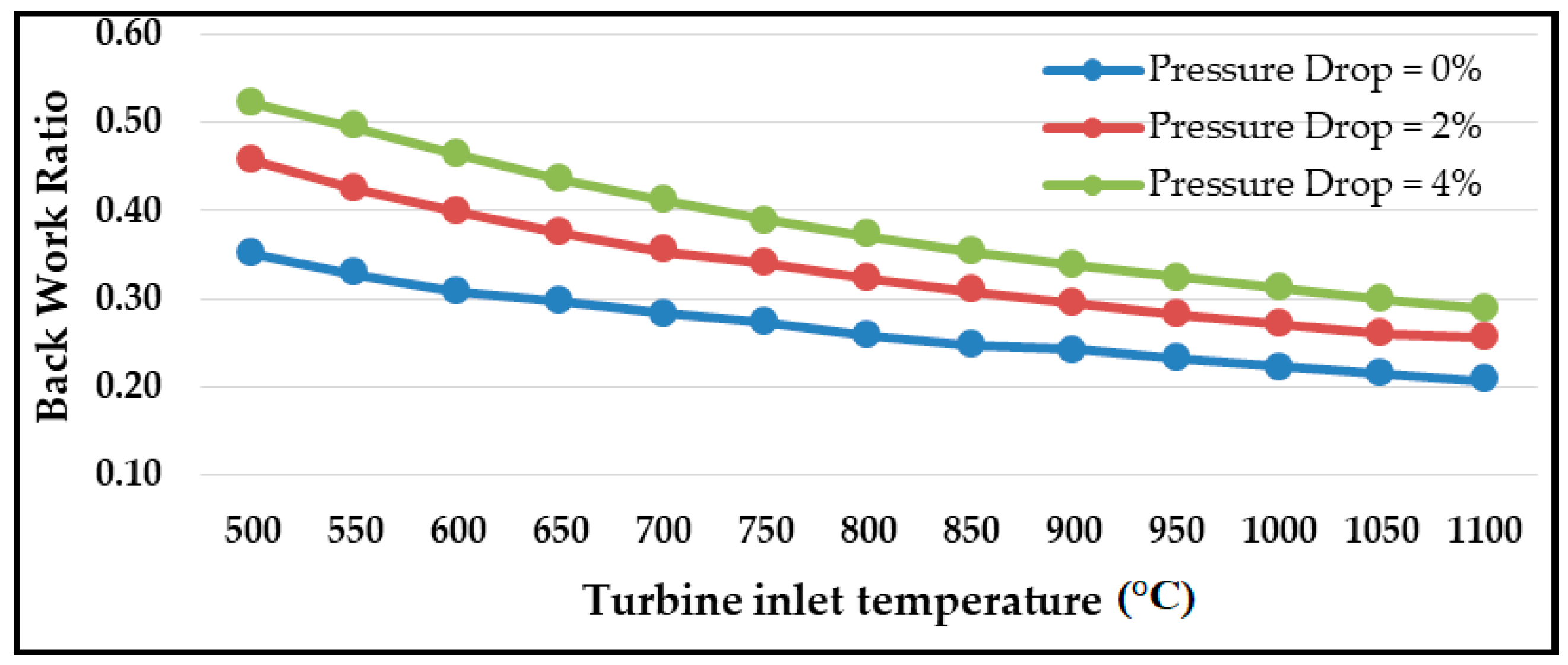
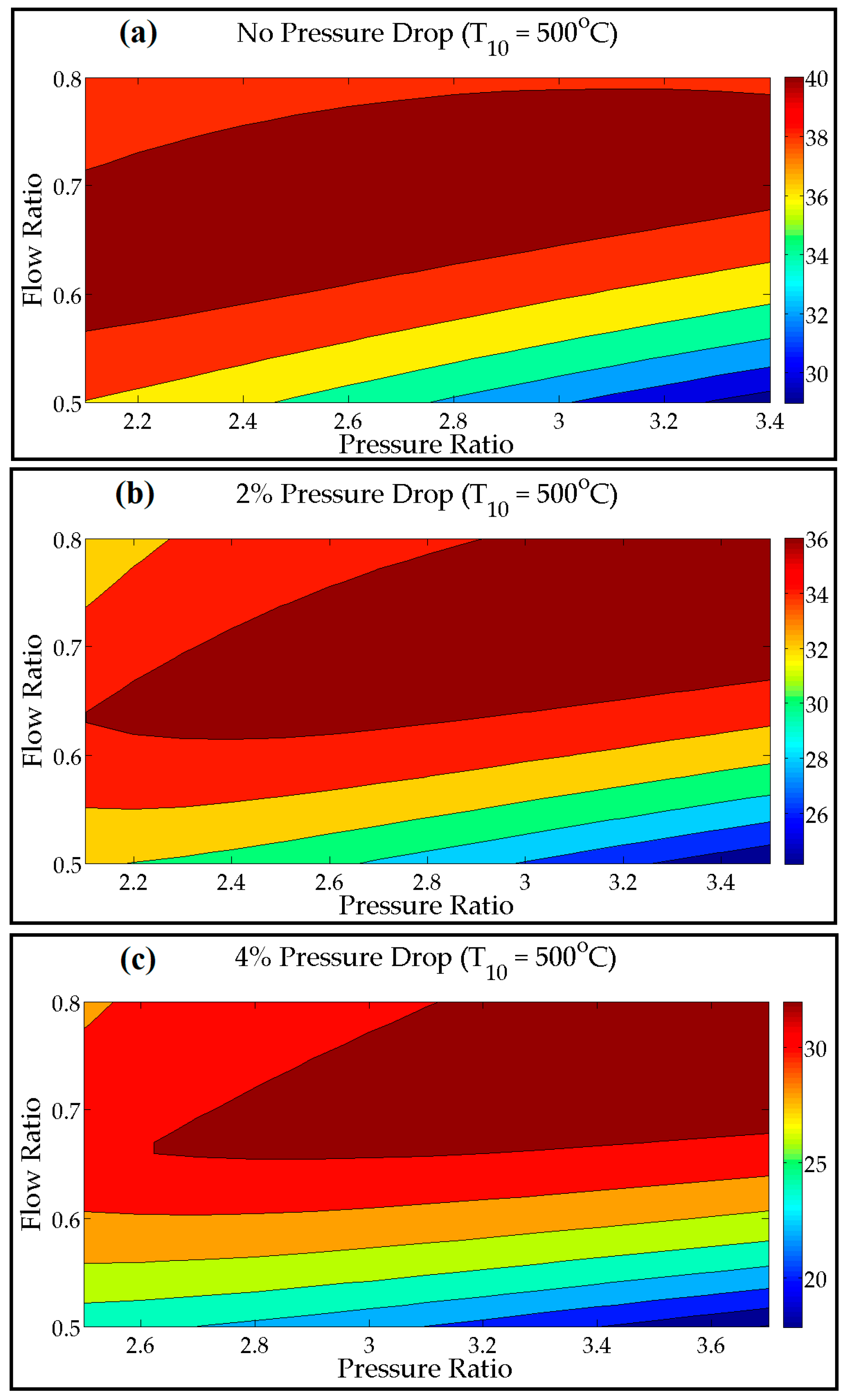
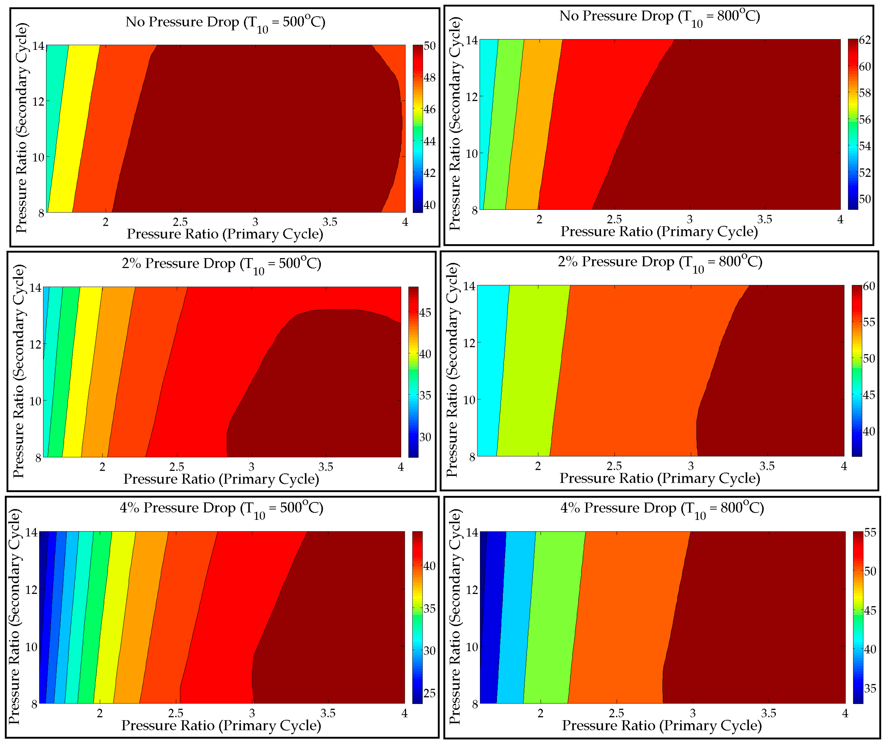
• As expected, the S-CO₂ RBC thermal efficiency declined with the pressure drop. The pressure drop in the heat exchangers resulted in increased compressor work required to maintain the optimum cycle pressure. The optimum cycle pressure was 16.60 MPa, which raised to 24.45 MPa for a 4% pressure drop.
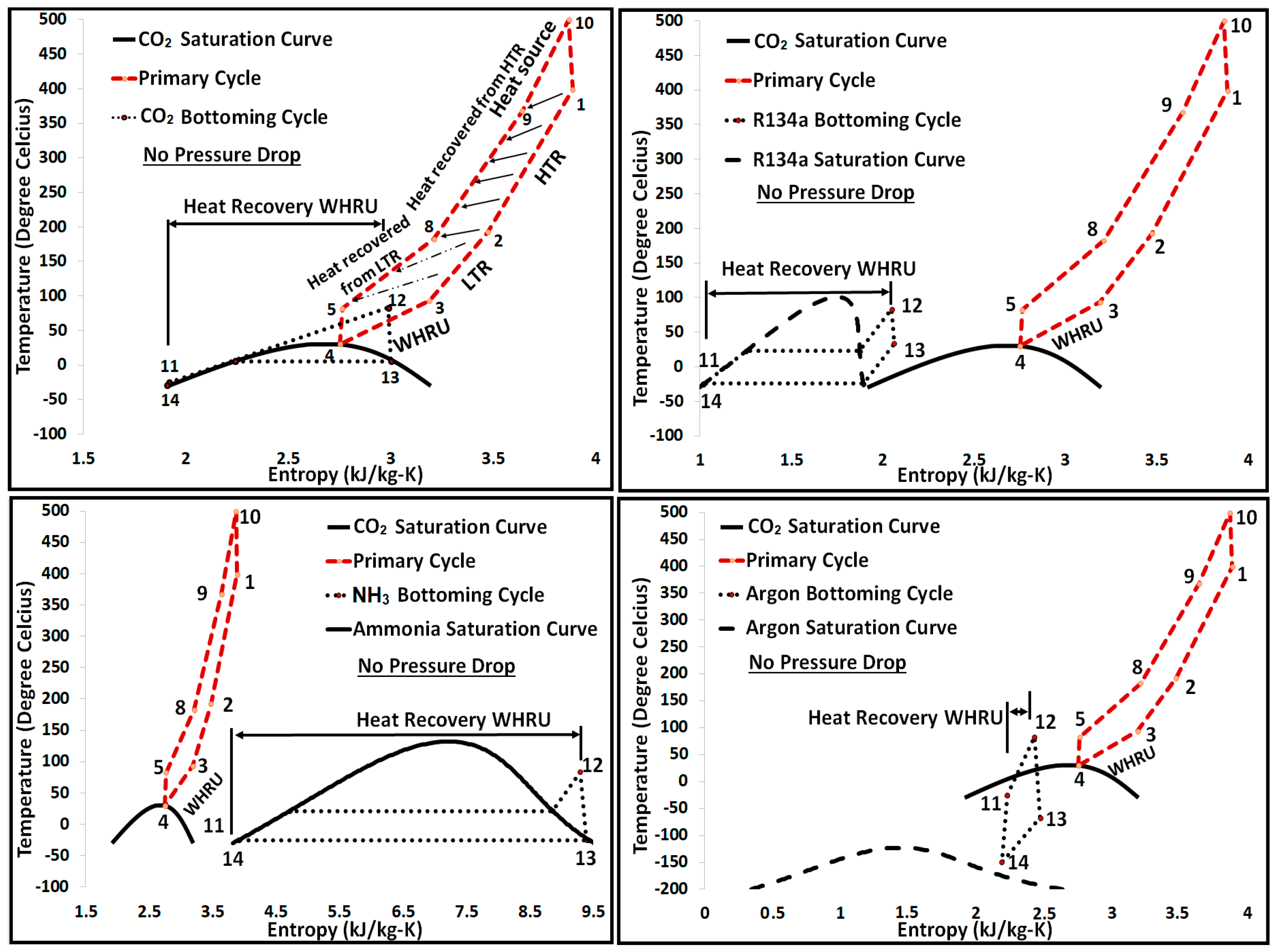
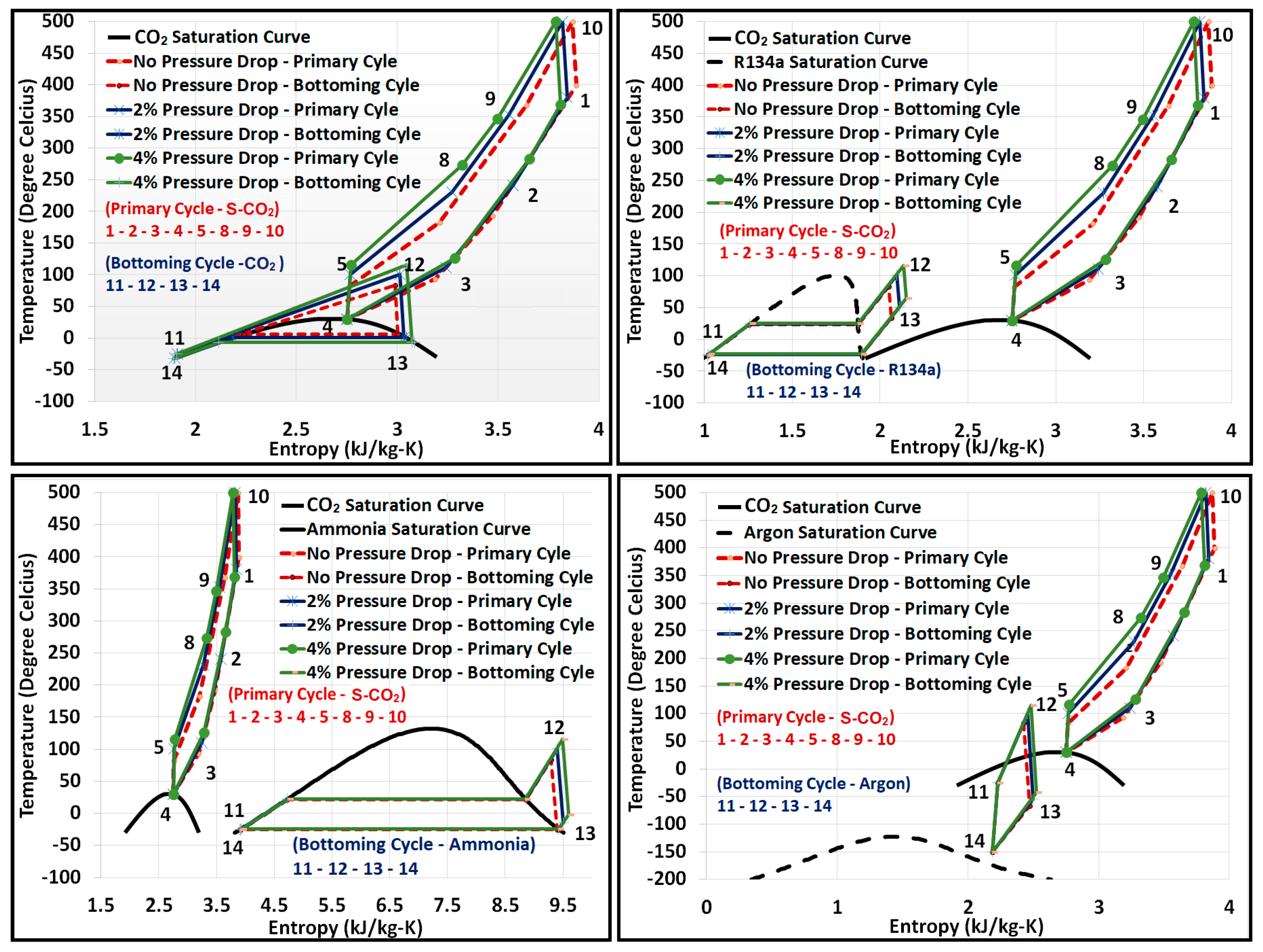
• Implementing the bottoming cycle is an attractive option with a sink temperature as low as −50 °C.
• The pressure drop in the primary cycle reduced the efficiency but, in turn, offered higher temperature and exergy available to the WHRU, which appeared as an increased contribution from the secondary cycle.
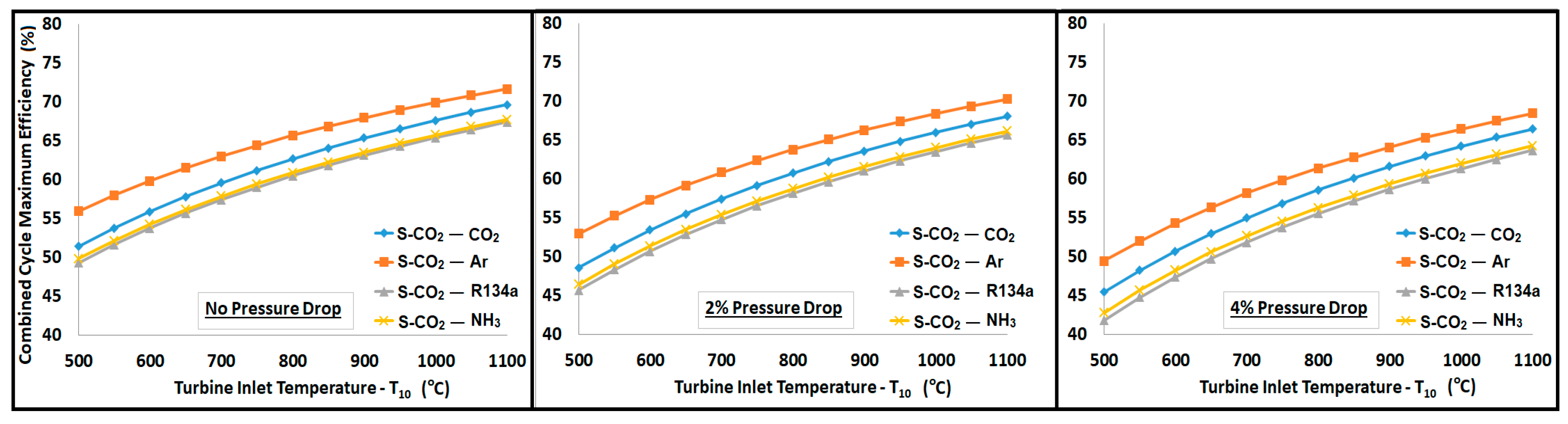
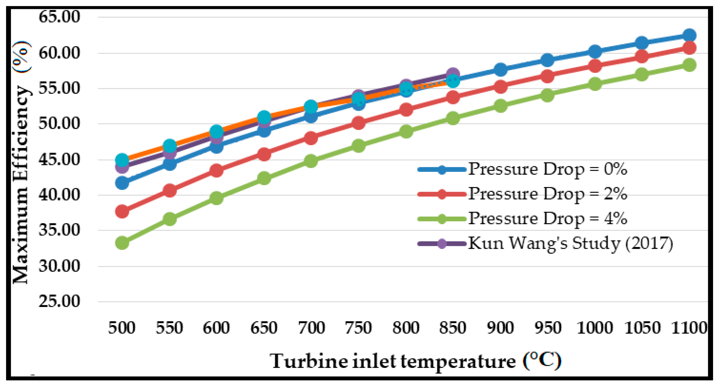
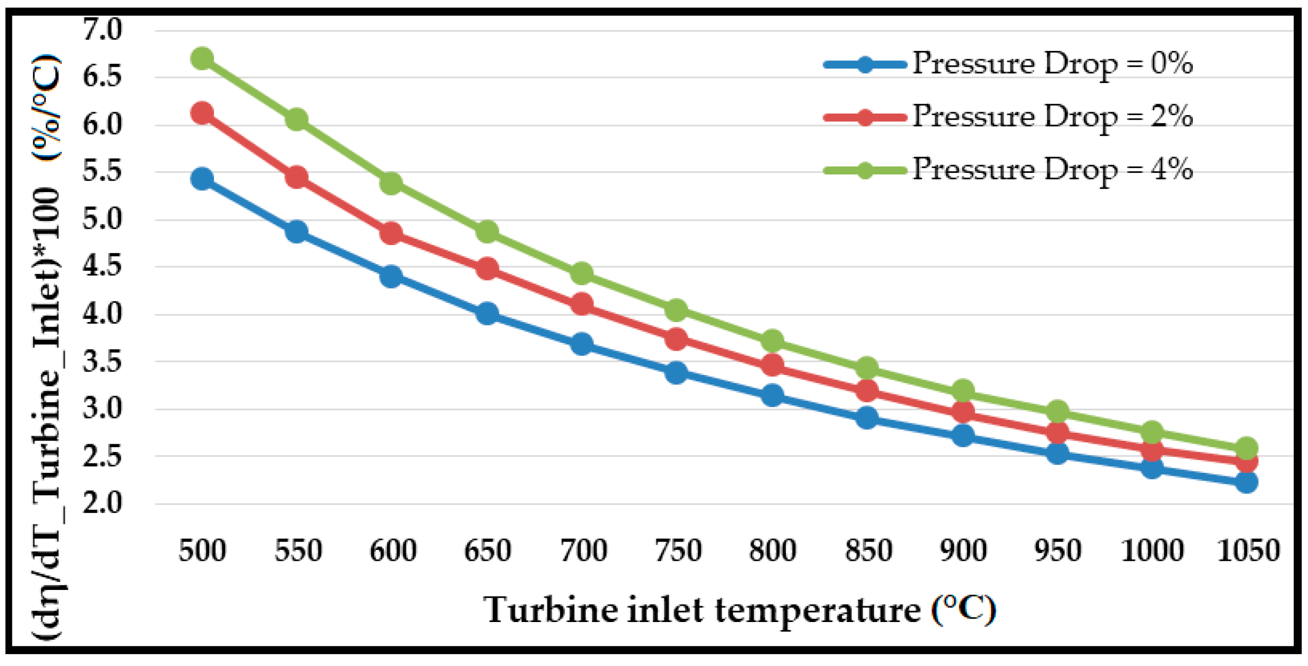
• The combined cycle efficiency increased monotonically with the turbine inlet temperature (T₁₀); the rise was more evident for temperatures up to 850 °C, beyond which the curve appeared to saturate.
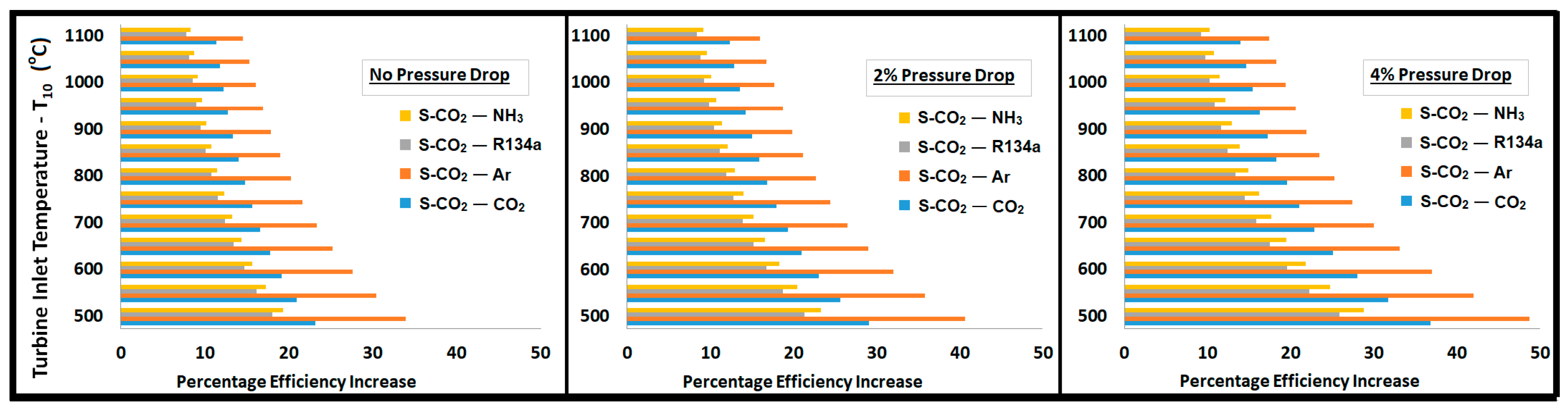
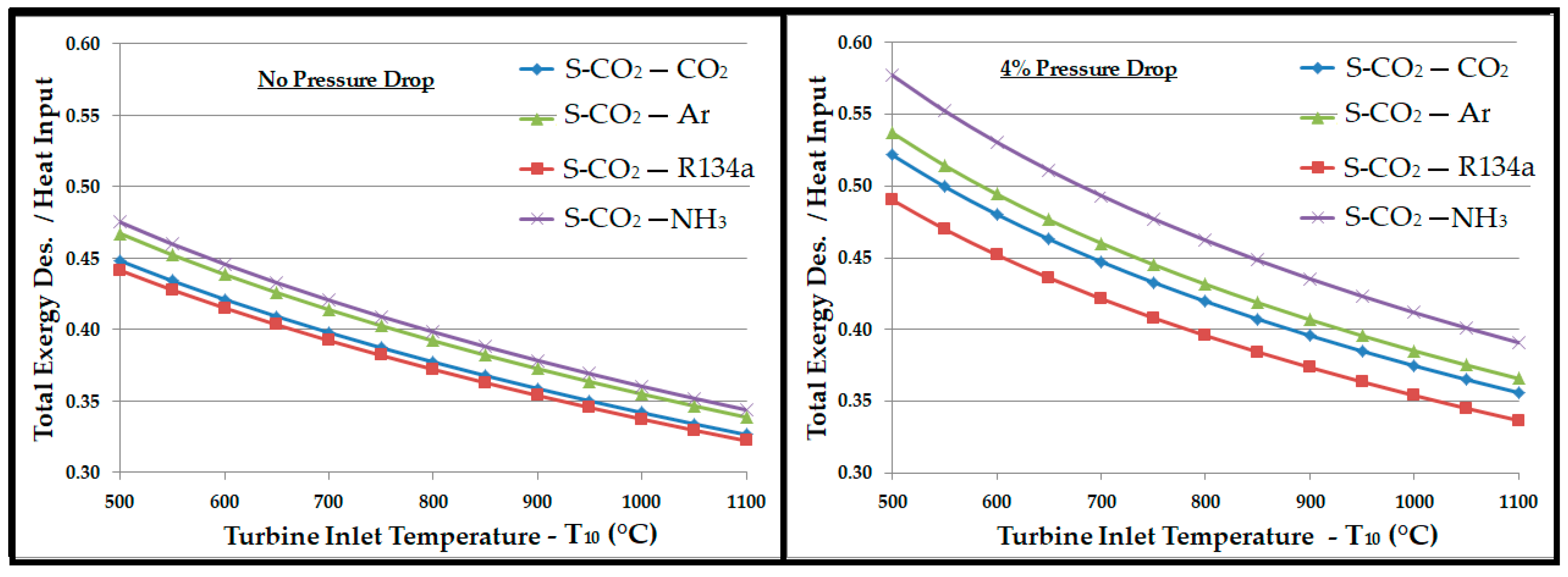
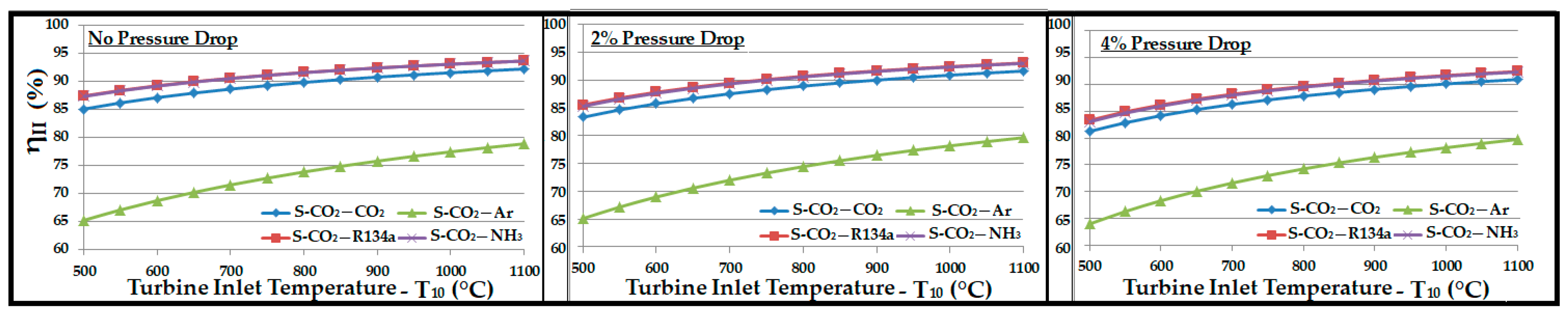
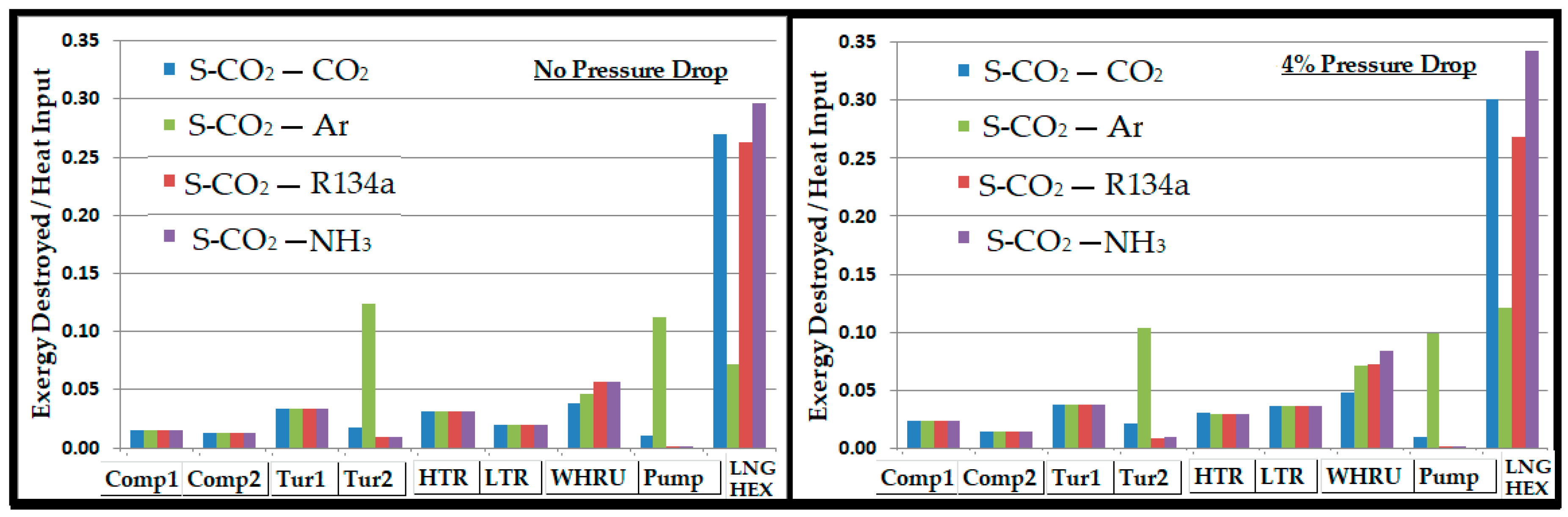
• Regardless of the pressure drop in the system, the bottoming cycle with argon as a working fluid gave the highest thermal efficiency. On the other side, it required a mass flow rate approximately 5 times higher than R134a and CO₂. A high mass flow rate would require a large equipment (turbine, compressor, heat exchangers, etc.), which ultimately increases the capital and operational costs. Significantly high exergy losses in compressor, turbine, and WHRU were also associated with argon, which was manifested by the smaller second law efficiency.
• Ammonia required a mass flow rate approximately 4 to 5 times lower than those of R134a and CO₂. Exergy analysis revealed a higher second law efficiency associated with ammonia. However, a substantial amount of exergy was lost in the WHRU as a result of the high latent heat of vaporization for ammonia. Thus, a significantly smaller exergy was available for the secondary cycle, which resulted in a smaller contribution in the overall thermal efficiency in comparison to other working fluids.
• R134a can be a good candidate for the bottoming cycle. It offered an overall thermal efficiency improvement between 20% and 25%, as shown in Figure 10. It showed minimum exergy loss and high second law efficiency.
• CO₂ provided a significantly higher contribution than ammonia and R134a in the overall cycle efficiency improvement, with a sink temperature of about −25 °C. It provided a thermal efficiency improvement of 30% to 35%.

Considering the above energy and exergy analyses, CO₂ could be a good option for a combined cycle with S-CO₂ being the primary cycle. R134a could be the second viable option as a working fluid for the bottoming cycle.

References

1. Chacartegui, R.; Sánchez, D.; Muñoz, J.M.; Sánchez, T. Alternative ORC bottoming cycles for combined cycle power plants. Appl. Energy 2009, 86, 2162–2170. [Google Scholar] [CrossRef]
2. Cao, Y.; Dai, Y. Comparative analysis on off-design performance of a gas turbine and ORC combined cycle under different operation approaches. Energy Convers. Manag. 2017, 135, 84–100. [Google Scholar] [CrossRef]
3. Wang, X.; Dai, Y. Exergoeconomic analysis of utilizing the transcritical CO2 cycle and the ORC for a recompression supercritical CO2 cycle waste heat recovery: A comparative study. Appl. Energy 2016, 170, 193–207. [Google Scholar] [CrossRef]
4. Santini, L.; Accornero, C.; Cioncolini, A. On the adoption of carbon dioxide thermodynamic cycles for nuclear power conversion: A case study applied to Mochovce 3 Nuclear Power Plant. Appl. Energy 2016, 181, 446–463. [Google Scholar] [CrossRef]
5. Conboy, T.; Pasch, J.; Fleming, D. Control of a supercritical CO2 recompression Brayton cycle demonstration loop. J. Eng. Gas Turbines Power 2013, 135, 111701. [Google Scholar] [CrossRef]
6. Conboy, T.; Wright, S.; Pasch, J.; Fleming, D.; Rochau, G.; Fuller, R. Performance characteristics of an operating supercritical CO2 Brayton cycle. J. Eng. Gas Turbines Power 2012, 134, 111703. [Google Scholar] [CrossRef]
7. Wang, J.; Huang, Y.; Zang, J.; Liu, G. Research Activities on Supercritical Carbon Dioxide Power Conversion Technology in China. In Proceedings of the ASEM Turbo Expo 2014: Turbine Technical Conference and Exposition, Dusseldorf, Germany, 16−20 June 2014. [Google Scholar]
8. Vesely, L.; Dostal, V.; Hajek, P. Design of Experimental Loop With Supercritical Carbon Dioxide. In Proceedings of the 2014 22nd International Conference on Nuclear Engineering, Prague, Czech Republic, 7−11 July 2014. [Google Scholar]
9. Angelino, G.; Colonna Di Paliano, P. Multicomponent working fluids for organic Rankine cycles (ORCs). Energy 1998, 23, 449–463. [Google Scholar] [CrossRef]
10. Astolfi, M.; Romano, M.C.; Bombarda, P.; Macchi, E. Binary ORC (Organic Rankine Cycles) power plants for the exploitation of medium-low temperature geothermal sources—Part B: Techno-economic optimization. Energy 2014, 66, 435–446. [Google Scholar] [CrossRef]
11. Chen, Y.; Lundqvist, P.; Johansson, A.; Platell, P. A comparative study of the carbon dioxide transcritical power cycle compared with an organic Rankine cycle with R123 as working fluid in waste heat recovery. Appl. Therm. Eng. 2006, 26, 2142–2147. [Google Scholar] [CrossRef]
12. Chen, H.; Goswami, D.Y.; Stefanakos, E.K. A review of thermodynamic cycles and working fluids for the conversion of low-grade heat. Renew. Sustain. Energy Rev. 2010, 14, 3059–3067. [Google Scholar] [CrossRef]
13. Al-Sulaiman, F.A.; Atif, M. Performance comparison of different supercritical carbon dioxide Brayton cycles integrated with a solar power tower. Energy 2015, 82, 61–71. [Google Scholar] [CrossRef]
14. Atif, M.; Al-Sulaiman, F.A. Energy and exergy analyses of solar tower power plant driven supercritical carbon dioxide recompression cycles for six different locations. Renew. Sustain. Energy Rev. 2017, 68, 153–167. [Google Scholar] [CrossRef]
15. Wang, K.; He, Y.L.; Zhu, H.H. Integration between supercritical CO2 Brayton cycles and molten salt solar power towers: A review and a comprehensive comparison of different cycle layouts. Appl. Energy 2017, 195, 819–836. [Google Scholar] [CrossRef]
16. Hou, S.; Wu, Y.; Zhou, Y. Performance analysis of the combined supercritical CO2 recompression and regenerative cycle used in waste heat recovery of marine gas turbine. Energy Convers. Manag. 2017, 151, 73–85. [Google Scholar] [CrossRef]
17. Wang, X.; Liu, Q.; Bai, Z.; Lei, J.; Jin, H. Thermodynamic analysis of the cascaded supercritical CO2 cycle integrated with solar and biomass energy. Energy Procedia 2017, 105, 445–452. [Google Scholar] [CrossRef]
18. Cao, Y.; Ren, J.; Sang, Y.; Dai, Y. Thermodynamic analysis and optimization of a gas turbine and cascade CO2 combined cycle. Energy Convers. Manag. 2017, 144, 193–204. [Google Scholar] [CrossRef]
19. Wang, J.; Wang, J.; Dai, Y.; Zhao, P. Thermodynamic analysis and optimization of a transcritical CO2 geothermal power generation system based on the cold energy utilization of LNG. Appl. Therm. Eng. 2014, 70, 531–540. [Google Scholar] [CrossRef]
20. Ahmadi, M.H.; Mehrpooya, M.; Pourfayaz, F. Thermodynamic and exergy analysis and optimization of a transcritical CO2 power cycle driven by geothermal energy with liquefied natural gas as its heat sink. Appl. Therm. Eng. 2016, 109, 640–652. [Google Scholar] [CrossRef]
21. Amini, A.; Mirkhani, N.; Pakjesm Pourfard, P.; Ashjaee, M.; Khodkar, M.A. Thermo-economic optimization of low-grade waste heat recovery in Yazd combined-cycle power plant (Iran) by a CO2 transcritical Rankine cycle. Energy 2015, 86, 74–84. [Google Scholar] [CrossRef]
22. Walnum, H.T.; Nekså, P.; Nord, L.O.; Andresen, T. Modelling and simulation of CO2(carbon dioxide) bottoming cycles for offshore oil and gas installations at design and off-design conditions. Energy 2013, 59, 513–520. [Google Scholar] [CrossRef]
23. Wu, C.; Yan, X.J.; Wang, S.S.; Bai, K.L.; Di, J.; Cheng, S.F.; Li, J. System optimisation and performance analysis of CO2 transcritical power cycle for waste heat recovery. Energy 2016, 100, 391–400. [Google Scholar] [CrossRef]
24. Qiang, W.; Yanzhong, L.; Jiang, W. Analysis of power cycle based on cold energy of liquefied natural gas and low-grade heat source. Appl. Therm. Eng. 2004, 24, 539–548. [Google Scholar] [CrossRef]
25. Kim, C.W.; Chang, S.D.; Ro, S.T. Analysis of the power cycle utilizing the cold energy of LNG. Int. J. Energy Res. 1995, 19, 741–749. [Google Scholar] [CrossRef]
26. Zhang, N.; Lior, N. A novel near-zero CO2 emission thermal cycle with LNG cryogenic exergy utilization. Energy 2006, 31, 1666–1679. [Google Scholar] [CrossRef]
27. Deng, S.; Jin, H.; Cai, R.; Lin, R. Novel cogeneration power system with liquefied natural gas (LNG) cryogenic exergy utilization. Energy 2004, 29, 497–512. [Google Scholar] [CrossRef]
28. Feher, E.G. The Supercritical thermodynamic power cycle. Energy Convers. 1968, 8, 85–90. [Google Scholar] [CrossRef]
29. Angelino, G. Carbon dioxide condensation cycles for power production. J. Eng. Gas Turbines Power 1968, 90, 287. [Google Scholar] [CrossRef]
30. Dostal, V.; Driscoll, M.J.; Hejzlar, P. A Supercritical Carbon Dioxide Cycle for Next Generation Nuclear Reactors. Tech. Rep. MIT-ANP-TR-100 2004, 1–317. Available online: http://web.mit.edu/22.33/www/dostal.pdf (accessed on 28 August 2018).
31. Ahn, Y.; Lee, J.; Kim, S.G.; Lee, J.I.; Cha, J.E.; Lee, S.W. Design consideration of supercritical CO2 power cycle integral experiment loop. Energy 2015, 86, 115–127. [Google Scholar] [CrossRef]
32. Wang, K.; He, Y.L. Thermodynamic analysis and optimization of a molten salt solar power tower integrated with a recompression supercritical CO2 Brayton cycle based on integrated modeling. Energy Convers. Manag. 2017, 135, 336–350. [Google Scholar] [CrossRef]
33. Turchi, C.S.; Ma, Z.; Neises, T.W.; Wagner, M.J. Thermodynamic study of advanced supercritical carbon dioxide power cycles for concentrating solar power systems. J. Sol. Energy Eng. 2013, 135, 041007. [Google Scholar] [CrossRef]
34. Kim, I.H.; No, H.C. Physical model development and optimal design of PCHE for intermediate heat exchangers in HTGRs. Nucl. Eng. Des. 2012, 243, 243–250. [Google Scholar] [CrossRef]
35. Neises, T.; Turchi, C. A comparison of supercritical carbon dioxide power cycle configurations with an emphasis on CSP applications. Energy Procedia 2013, 49, 1187–1196. [Google Scholar] [CrossRef]
Figure 1. Schematic diagram of the supercritical carbon dioxide (S-CO2) recompression Brayton cycle. HTR: high-temperature recuperator; LTR: low-temperature recuperator.
Processes 06 00153 g001
Figure 2. Schematic diagram of the S-CO2 cycle coupled with a bottoming cycle. The dashed lines encircle the secondary or bottoming cycle. LNG: liquefied natural gas; HEX: heat exchanger.
Processes 06 00153 g002
Figure 3. (a) Contour plot of the thermal efficiency of the primary cycle for the no-pressure-drop condition plotted as a function of the flow ratio and pressure ratio for a turbine inlet temperature of 500 °C. (b) Contour plot of the thermal efficiency of the primary cycle for the 2% pressure drop condition plotted as a function of the flow ratio and pressure ratio for a turbine inlet temperature of 500 °C. (c) Contour plot of the thermal efficiency of the primary cycle for the 4% pressure drop condition plotted as a function of flow ratio and pressure ratio for a turbine inlet temperature of 500 °C.
Processes 06 00153 g003
Figure 4. Temperature–entropy (T–S) diagram of the primary cycle (S-CO2 recompression Brayton cycle (RBC)) plotted for a turbine inlet temperature of 500 °C. All state points correspond to the numbers shown in Figure 1.
Processes 06 00153 g004
Figure 5. Thermal efficiency of the primary cycle plotted against turbine inlet temperature for the no-pressure-drop, the 2% pressure drop, and the 4% pressure drop conditions. Data points taken from references [32,35] are also plotted for comparison.
Processes 06 00153 g005
Figure 6. Back work ratio of the primary cycle plotted as a function of turbine inlet temperature for the no-pressure-drop, the 2% pressure drop, and the 4% pressure drop conditions. For all cases, the back work ratio decreases with the increase of the turbine inlet temperature.
Processes 06 00153 g006
Figure 7. Change in the cycle’s thermal efficiency per unit change in turbine inlet temperature plotted as a function of turbine inlet temperature for the no-pressure-drop, the 2% pressure drop, and the 4% pressure drop conditions. For all cases, the improvement in the cycle’s thermal efficiency declines with the increase of then turbine inlet temperature.
Processes 06 00153 g007
Figure 8. Contour plots of the thermal efficiency of the combined cycle as a function of pressure ratios of the primary and secondary cycles for turbine inlet temperatures of (left) 500 °C and (right) 800 °C in (top) the no-pressure-drop condition, (center) the 2% pressure drop condition, and (bottom) the 4% pressure drop condition. CO2 is considered as the working fluid in the secondary cycle.
Processes 06 00153 g008
Figure 9. Thermal efficiency of the combined cycle plotted against the turbine inlet temperature (T10) for (left) the no-pressure-drop condition, (center) the 2% pressure drop condition, and (right) the 4% pressure drop condition. For all cases, the cycle’s thermal efficiency monotonically increases with the turbine inlet temperature; the S-CO2–Argon cycle appears the most efficient.
Processes 06 00153 g009
Figure 10. Improvement in the thermal efficiency of the combined cycle (in percentage) in comparison to the standalone S-CO2 cycle plotted against the turbine inlet temperature (T10)) for (left) the no-pressure-drop condition, (center) the 2% pressure drop condition, and (right) the 4% pressure drop condition.
Processes 06 00153 g010
Figure 11. T–S plots of the S-CO2 cycle coupled with the secondary (top left) CO2 cycle, (top right) R134a cycle, (bottom left) ammonia cycle, and (bottom right) argon cycle. No pressure drop is considered.
Processes 06 00153 g011
Figure 12. Effect of pressure drop on the T–S plots of the S-CO2 cycle coupled with the secondary (top left) CO2 cycle, (top right) R134a cycle, (bottom left), ammonia cycle and (bottom right), argon cycle.
Processes 06 00153 g012
Figure 13. Exergy destroyed (normalized by heat input) in various components of the combined cycle plotted for (left) the no-pressure-drop condition and (right) the 4% pressure drop condition with a turbine inlet temperature of T10 = 500 °C.
Processes 06 00153 g013
Figure 14. Total exergy destruction (normalized by heat input) plotted as a function of turbine inlet temperature for each combined cycle for (left) the no-pressure-drop condition and (right) the 4% pressure drop condition. For all cases, total exergy destruction exhibits a monotonically decreasing behavior with the turbine inlet temperature.
Processes 06 00153 g014
Figure 15. Second law efficiency of the combined cycle plotted as a function of turbine inlet temperature for (left) the no-pressure-drop condition, (center) the 2% pressure drop condition, and (right) the 4% pressure drop condition. For all cases, argon stands out as the least efficient candidate.
Processes 06 00153 g015