On-Line Optimal Input Design Increases the Efficiency and Accuracy of the Modelling of an Inducible Synthetic Promoter ^†

Abstract

Synthetic biology seeks to design biological parts and circuits that implement new functions in cells. Major accomplishments have been reported in this field, yet predicting a priori the in vivo behaviour of synthetic gene circuits is major a challenge. Mathematical models offer a means to address this bottleneck. However, in biology, modelling is perceived as an expensive, time-consuming task. Indeed, the quality of predictions depends on the accuracy of parameters, which are traditionally inferred from poorly informative data. How much can parameter accuracy be improved by using model-based optimal experimental design (MBOED)? To tackle this question, we considered an inducible promoter in the yeast S. cerevisiae. Using in vivo data, we re-fit a dynamic model for this component and then compared the performance of standard (e.g., step inputs) and optimally designed experiments for parameter inference. We found that MBOED improves the quality of model calibration by ∼60%. Results further improve up to $84\%$ when considering on-line optimal experimental design (OED). Our in silico results suggest that MBOED provides a significant advantage in the identification of models of biological parts and should thus be integrated into their characterisation.

1. Introduction

Synthetic biology, a discipline at the interface of biology, engineering and computer science, seeks to engineer cells with new functionalities. Despite great progress towards this goal [1], the prediction of the in vivo behaviour of synthetic circuits is still a challenge that hinders technological applications. For the field to reach its full potential, the accurate prediction of the dynamics of synthetic circuits needs to be achieved. Mathematical models can serve as a tool to gain a mechanistic understanding of a system and could tackle this issue; however, their adoption in synthetic biology has so far been limited [2]. Indeed, while biophysical and static models have been successfully proposed as tools to guide the automated design of biological circuits [3,4], the use of mathematical models is often confined to the interpretation of experimental data.

The lack of widespread use of mathematical models can be attributed to the limited availability of extensively characterised biological components, the often neglected contextual dependence of the behaviour of circuits [5] and the difficulty of estimating unknown parameters of large multipart systems from input–output data. The latter, usually sparse and noisy, are traditionally acquired using experimental platforms (e.g., microplate readers) which pose constraints towards flexible experimental designs. “Pulses” or “steps” of chemicals are the de facto standard stimuli to probe part behaviour. Unfortunately, such designs often yield poorly-informative data. Indeed, these inputs are low-pass filtered by molecular diffusion, which limits their frequency content. Furthermore, while persistent excitation is proven optimal to identify linear systems [6], there is not such a general result for non-linear systems such as biological networks. The question is then, is it possible to design experiments to identify models that predict the behaviour of biological circuits, and if so, how?

Model-based Optimal Experimental Design (MBOED) allows the design of experiments with maximal information content for parameters inference. Previous works addressed the potential of using MBOED in biological systems. Bandara et al. [7] considered a cell signalling example and showed that optimally designed experiments supported a 60-fold decrease in the variance of parameter estimates when compared to intuition driven designs. Similarly, Ruess et al. showed how optimised dynamic inputs outperformed random inputs in characterising a light-inducible promoter [8].

Despite these promising results, in general, the synthetic biology community has not adopted MBOED. Among the reasons: optimally designed experiments are difficult to implement with traditional experimental platforms and the skills to design them are not widespread in wet laboratories. Technological developments (e.g., microfluidics) and software tools (e.g., AMIGO2 [9]) help to alleviate these problems but they have steep learning curves. Is MBOED worth the extra effort of adoption?

This work addresses this question by identifying a mathematical model of a building block in synthetic biology: an inducible promoter. Many synthetic promoters use DNA sequences from the same organism for which they are engineered, and so potentially suffer from unwanted regulation from other genes in the genome. This additional regulation makes disentangling and modelling promoter activity a challenge. To overcome such issues, we considered an orthogonal promoter [10], i.e., a S. cerevisiae promoter engineered with DNA sequences from E. coli. The promoter, designed by Gnügge et al. [10] (Figure 1), controls the expression of a fluorescent reporter, Citrine, when cells sense the chemical IPTG. IPTG permeates the cell through the heterologous transporter Lac12 and binds the LacI repressor, thereby relieving its downregulation on promoter activity. Binding of the constitutively expressed tTA to the tetO${}_2$ site leads to the expression of Citrine.

As a first step, we refined a mathematical model of the inducible promoter ($M_{PLac}$), obtaining $M_{PLac,r}$ using available data [10]. We then proposed a simplified model structure, ${\mathcal{M}}_{3D}$, able to mimic the dynamics of $M_{PLac,r}$ ($M_{IP,r}$). We compared the performance of optimal and intuition-driven input profiles for the identification of $M_{IP,r}$ using the posterior distributions of the inferred parameters. Finally, we assessed the improvement of on-line MBOED over off-line MBOED as quantified by the accuracy of the estimates and their convergence rate to the actual parameter values. Note that, while in off-line MBOED the optimised input was computed for the entire experiment before this begins, on-line MBOED was characterised by iterative, data-informed refinements of both the model and stimulus profile within a single experiment.

Our results suggest that iterative off-line and on-line MBOED enable the design of more informative experiments for the characterisation of biological parts, e.g., synthetic promoters. Furthermore, we quantify the increase in the confidence of the inferred parameter estimates. The manuscript is organised as follows: Section 2 discusses how we recalibrate a model of the inducible promoter, define a reduced model and use it to compare the information content of different input classes. The section closes with a comparison between off-line and on-line MBOED schemes. Section 3 expands on the importance of MBOED for the design of more informative experiments in synthetic biology. Section 4 details our in silico experiments, the comparison of information content of different input classes and the design of optimal experiments. Finally, Section 5 presents our conclusions and future directions.

2. Results

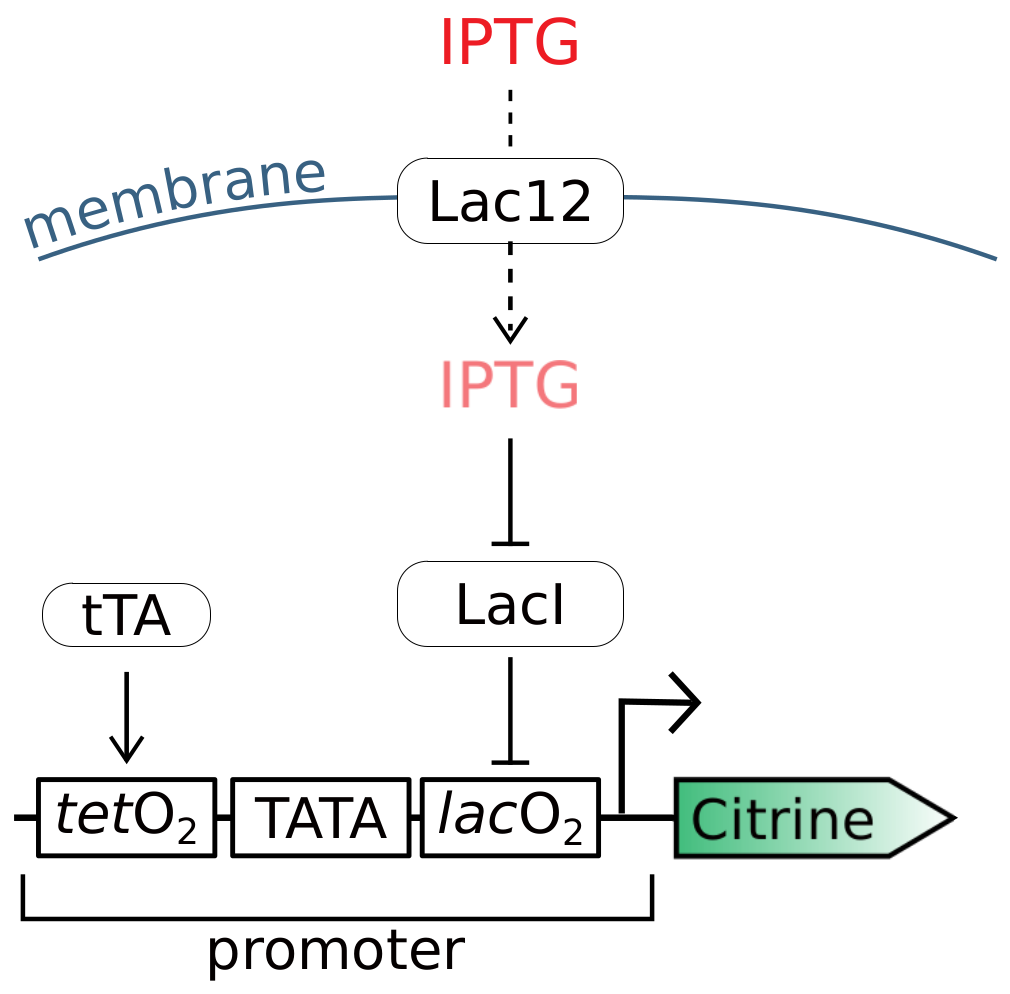
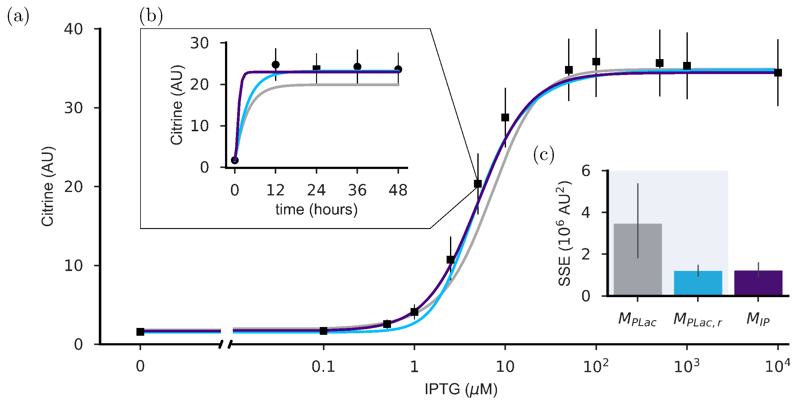
2.1. Refitting Gnügge et al.’s Model

First, we recovered $M_{PLac}$, the model published by Gnügge and colleagues [10], and independently assessed its ability to describe the experimental data reported in the original paper [10]. The dataset includes 24 IPTG dose–response curves (five samples, 12 h intervals). Our analysis reveals that $M_{PLac}$ consistently underestimates by 20–30% the steady states at intermediate concentrations (Figure 2, grey line).

To resolve this discrepancy, we set out to recalibrate $M_{PLac}$ using enhanced Scatter Search (eSS) [11]. The new model, $M_{PLac,r}$ (Figure 2a, cyan) generally better recapitulates the experimental data (Figure 2b). Quantitatively, $M_{PLac,r}$ achieved a 56% improvement in fit accuracy—quantified as the sum of squared errors (SSE) of predictions (Figure 2c).

2.2. The Dynamics of the Inducible Promoter Is Captured by a Reduced-Order Model

We developed a reduced order model structure (${\mathcal{M}}_{3D}$) to constrain the number of parameters to be identified as well as the computational cost associated with optimal experimental design. The model structure reads as follows:

$${\mathcal{M}}_{3D}=\left\{\begin{array}{cc}{\displaystyle \frac{dR}{dt}}\hfill & =\alpha +v\frac{IPT{G}^h}{K_r^h+IPT{G}^h}-\gamma R\hfill \\ \frac{d{P}_f}{dt}\hfill & =k_{p}R-({\gamma }_f+k_f)P_f\hfill \\ \frac{d{P}_m}{dt}\hfill & =k_f{P}_f-{\gamma }_f{P}_m,\hfill \end{array}\right.$$

where R, $P_f$ and $P_m$ are the concentrations of Citrine mRNA, immature folded protein and matured (fluorescent) protein, respectively. The model encompasses transcription, translation and maturation of the fluorescent reporter and has eight parameters. Transcription depends on the concentration of the inducer IPTG through a Michaelis–Menten kinetics, where v is the maximal induced transcriptional rate; h the Hill coefficient; $K_r$ the Michaelis–Menten constant; and $\alpha$ is the basal transcription. Translation occurs at a rate $k_p$ and the folded protein matures at rate $k_f$. All biochemical species are subject to linear degradation, occurring at rates $\gamma$ for mRNA and ${\gamma }_f$ for protein. The ${\mathcal{M}}_{3D}$ model structure builds on the assumption of time-scale separation between the expression of the repressor LacI, its dimerisation and subsequent binding to the operator sites and to IPTG, which are considered at quasi steady state, and Citrine expression. Calibrating ${\mathcal{M}}_{3D}$ to the time-series data in [10], we obtained $M_{IP}$.

We observed that $M_{IP}$ better fits both the steady-states, i.e., the dose–response curve (Figure 2a), and the dynamics of the system (see Figure 2b for an example). Despite its lower order, $M_{IP}$ achieved predictive capabilities comparable to $M_{PLac,r}$ considering the sum of squared errors over the whole set of experimental data (Figure 2c). It is worth noting that $M_{IP}$ is characterised by a smaller rise time (1.8 h) than both $M_{PLac}$ and $M_{PLac,r}$ (7.9 h) (Figure 2b). Here, the rise time is defined as the time taken by the output to rise from 10% to 90% of the steady-state. Unfortunately, the low sampling frequency used in the original study [10] impeded any further constraints on the characteristic time-scale of the system.

As we aimed to explore the informative content of different input classes (Section 2.3), we required our reduced model to closely mirror the dynamics of the considered inducible promoter. We therefore used $M_{PLac,r}$ to produce a set of pseudo-experimental data to re-calibrate $M_{IP}$, thereby obtaining $M_{IP,r}$. While $M_{IP}$ could have been selected as a nominal model for MBOED, the possibility of expanding the available dataset and further constraining model calibration made us prefer $M_{PLac,r}$ as a reference. The limited complexity of the underlying biological system prompted us to adopt stepwise, pulses, ramp-wise and stepwise random inputs in the generation of the pseudo-data (Section 4.1). The results of $M_{IP,r}$ parameterization show that this model mimics the dynamics of $M_{PLac,r}$ (Figure 3).

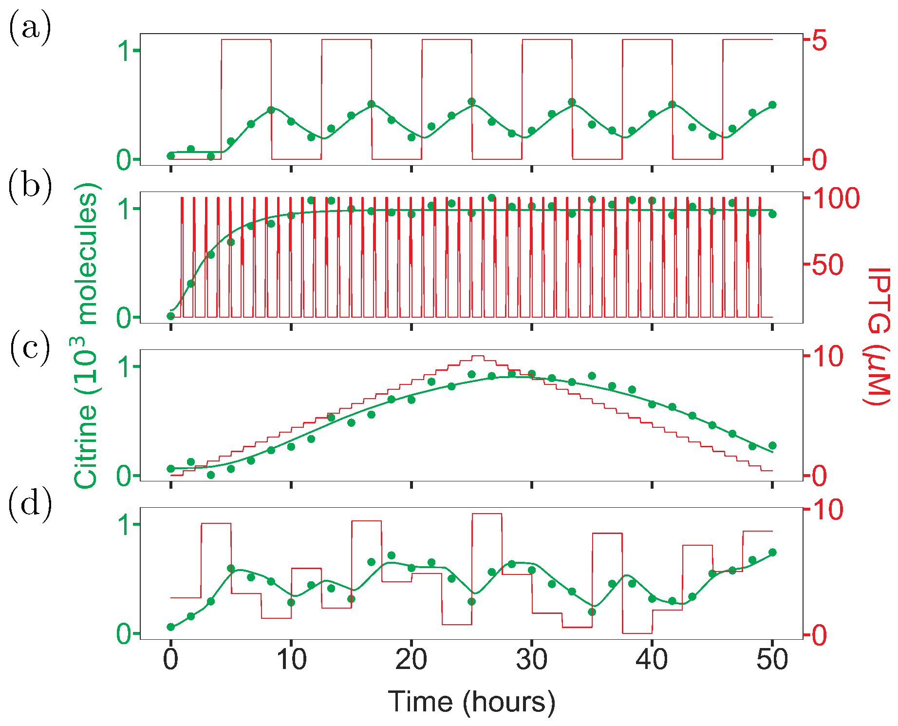
2.3. Intuition-Driven Inputs Are Poorly Informative

We next aimed to compare the performance of intuition-driven stimuli (step, pulse and random) for the parameterisation of ${\mathcal{M}}_{3D}$. We generate $N_j$ = 100 stimulation patterns for each of the three classes (Section 4.2). By simulating the response of $M_{IP,r}$ to each input, we collected pseudo-experimental data to inform the calibration of ${\mathcal{M}}_{3D}$. We cast parameter estimation as a non-linear optimisation problem and addressed it using eSS [11]. The use of standard metrics (e.g., z-score) to quantify the statistical significance of the distance between nominal and estimated parameter values was ruled out by the parameter posteriors not following a normal distribution. To overcome this limitation, we defined the relative error, ${\epsilon }_i^{\left(j\right)}$, between each parameter estimate, $p_i^{\left(j\right)}$, and its true value, $p_i^{*}$:

$${\epsilon }_i^{\left(j\right)}=\left|{log}_2\left(\frac{p_i^{\left(j\right)}}{p_i^{*}}\right)\right|$$

(1)

where i identifies the $i^{th}$ entry in the parameter vector and j is the index of the input profile yielding the parameter estimate $p_i^{\left(j\right)}$. Note that ${\epsilon }_i^{\left(j\right)}=0$ when the parameter estimate equals its true value, while the absolute value ensures equal treatment of under- and over-estimates.

In Figure 4, the distributions of relative error for the 100 input profiles highlight a differential sensitivity of the output to the parameters (Figure 4b–d). We note that the high dispersion in the estimates of $\alpha$, v and $\gamma$ aligns with a preliminary analysis of practical identifiability (results not shown), which suggested a high correlation between these parameters. Practical identifiability issues can indeed hamper the accuracy of the estimates of the affected parameters. Interestingly, the ${\epsilon }_i$ distributions advocate that the intuition-driven inputs convey a similar amount of information (Figure 4b–d). This was further confirmed by the absence of statistically significant difference in the average relative error ($\overline{\epsilon }$) (Figure 4f), defined as:

$$\overline{\epsilon }=\frac{1}{N_p{N}_j}\sum _{i=1}^{N_p}\sum _{j=1}^{N_j}{\epsilon }_i^{\left(j\right)}$$

(2)

where $N_p$ is the number of parameters in the model structure and $N_j$ is the number of input profiles.

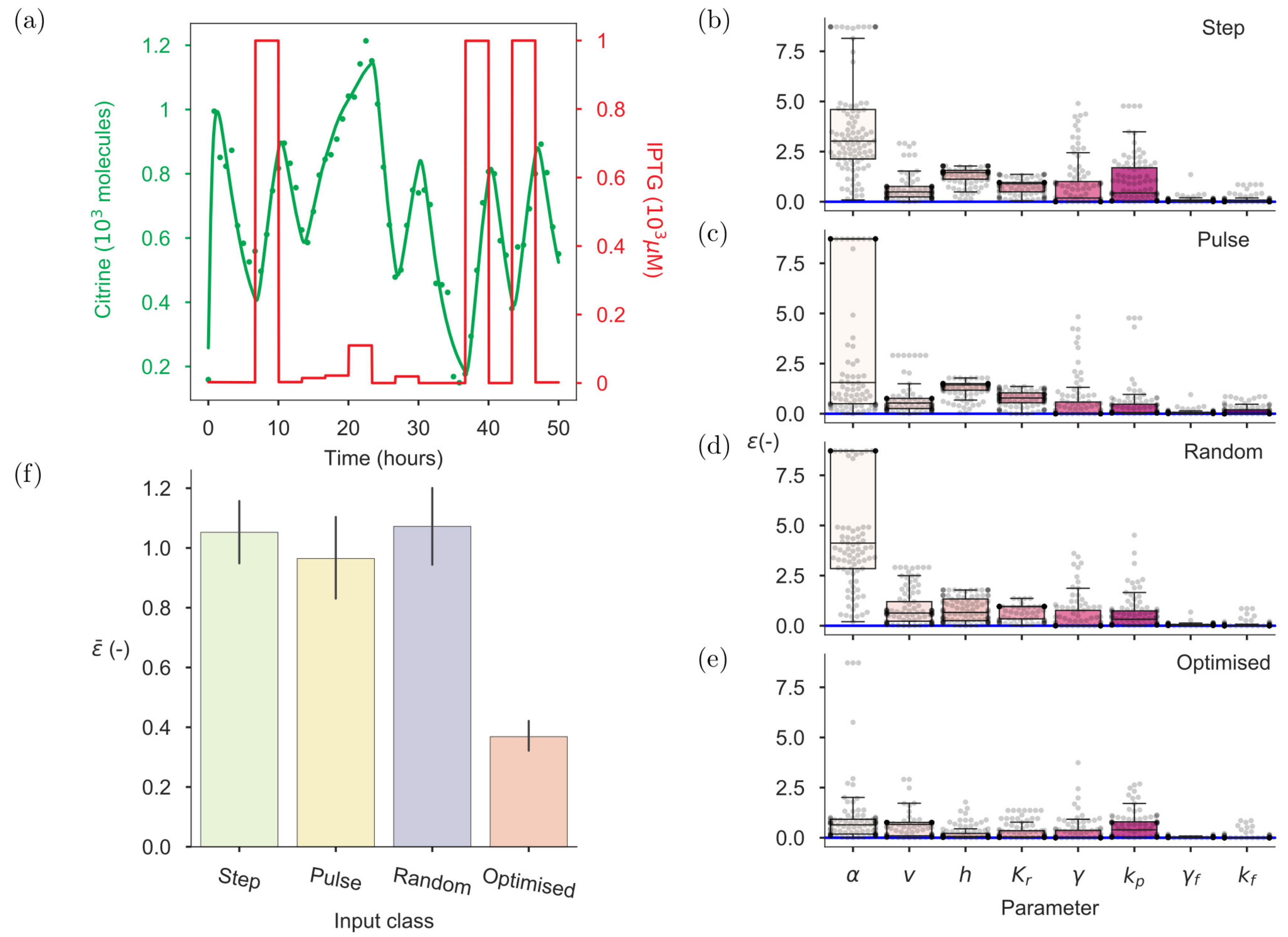
2.4. Optimal Input Design (OID) Increases the Accuracy of Model Identification

Next, we questioned the improvement in the accuracy of parameter inference enabled by optimally designed experimental schemes. To reflect wet-lab experimental constraints, originating from the assumption of using a microfluidic-based platform, and to compare the informative content of intuition-driven and optimised inputs under similar conditions, we set the duration of the experiment to 3000 min and the sampling intervals to 5 min. Furthermore, we assumed a constant duration of 200 min for the steps in the optimised input (Section 4.4). Consequently, we formulated OID as a constrained optimisation problem that searches for the IPTG concentrations, (i.e., amplitude of the steps of IPTG) that maximise the information content. The optimisation relies here on the D-optimality criterion [12], which seeks to maximise the determinant of the Fisher Information Matrix ($\mathcal{F}$) [6,13]. We designed $N_j$ = 100 optimised stimulation profiles (see Figure 4a for an example), applied them to $M_{IP,r}$ to generate pseudo-data and performed model calibration. In our results, the use of optimised inputs enabled a noticeable reduction in $\epsilon$ compared to intuition-based inputs (Figure 4b–e). The higher confidence of parameter estimates even for the poorly identifiable parameters $\alpha$, v and $\gamma$, translated to a 64% reduction in $\overline{\epsilon }$ for the optimally designed input over the intuition-driven counterparts.

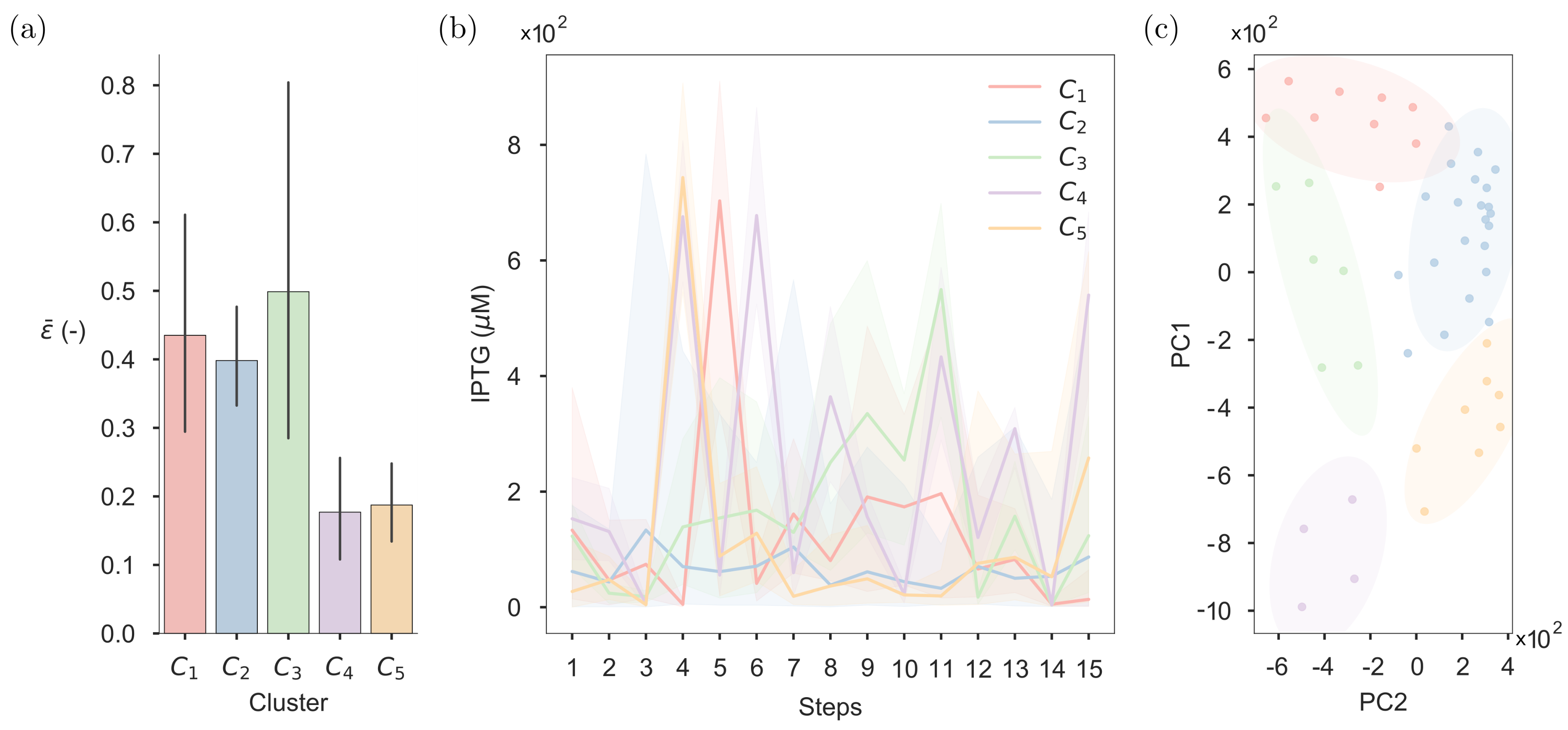
2.5. Clustering of the Optimised Inputs

To explore the properties of the optimised stimulation profiles and their effect on the accuracy of parameter estimates, we clustered the 15-dimensional input space through Self-Organising Maps (SOM) [14]. Specifically, the $N_j$ = 100 optimally designed inputs were projected on 49 vector prototypes or nodes using the SOM Toolbox [15] (Section 4.5). Hence, the nodes were grouped using agglomerative, hierarchical clustering. Both the silhouette and the Calinksi–Harabasz internal validity index [16] suggested an optimal partitioning of the dataset into five clusters. In Figure 5, the accuracy of parameter inference, as quantified by the average relative error ($\overline{\epsilon }$) for the inputs assigned to each group, proved to be cluster-specific (Figure 5a). As the observed differences could not be ascribed to the correlation between $\overline{\epsilon }$ and the value of the objective function attained by the optimiser, we investigated the pattern of IPTG values of the prototype vectors. This analysis revealed that the best performing clusters, $C_4$ and $C_5$, are characterised by a high inducer concentration after 10 h of stimulation (Figure 5b). It is worth noting that, despite the system being initially in an uninduced state, the optimiser selected low IPTG values in the first steps: a counter-intuitive choice for an experimentalist.

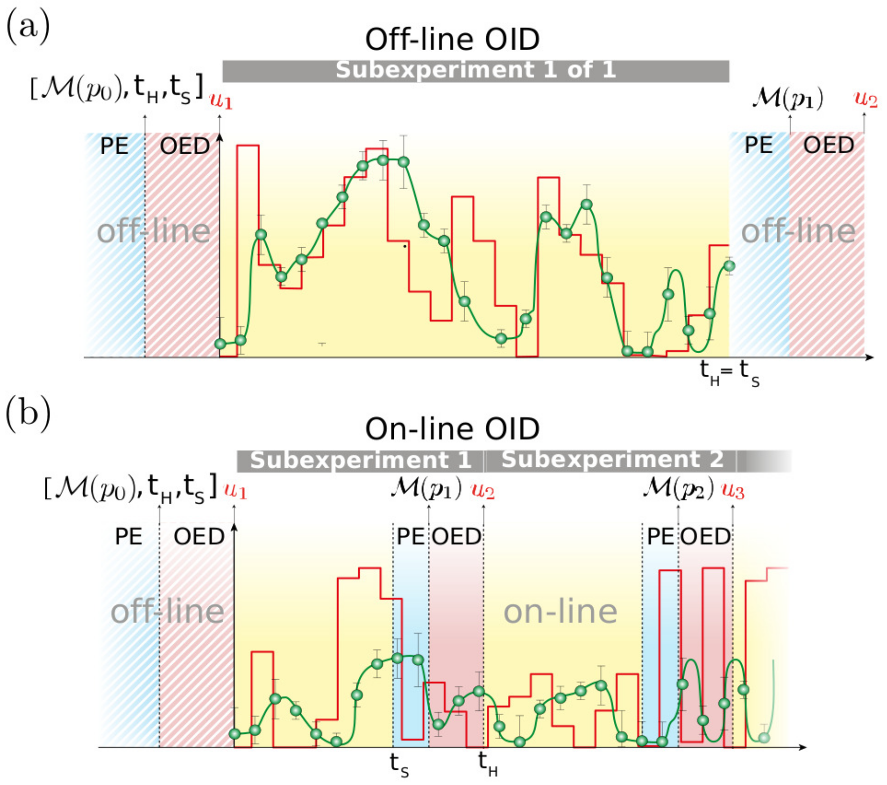
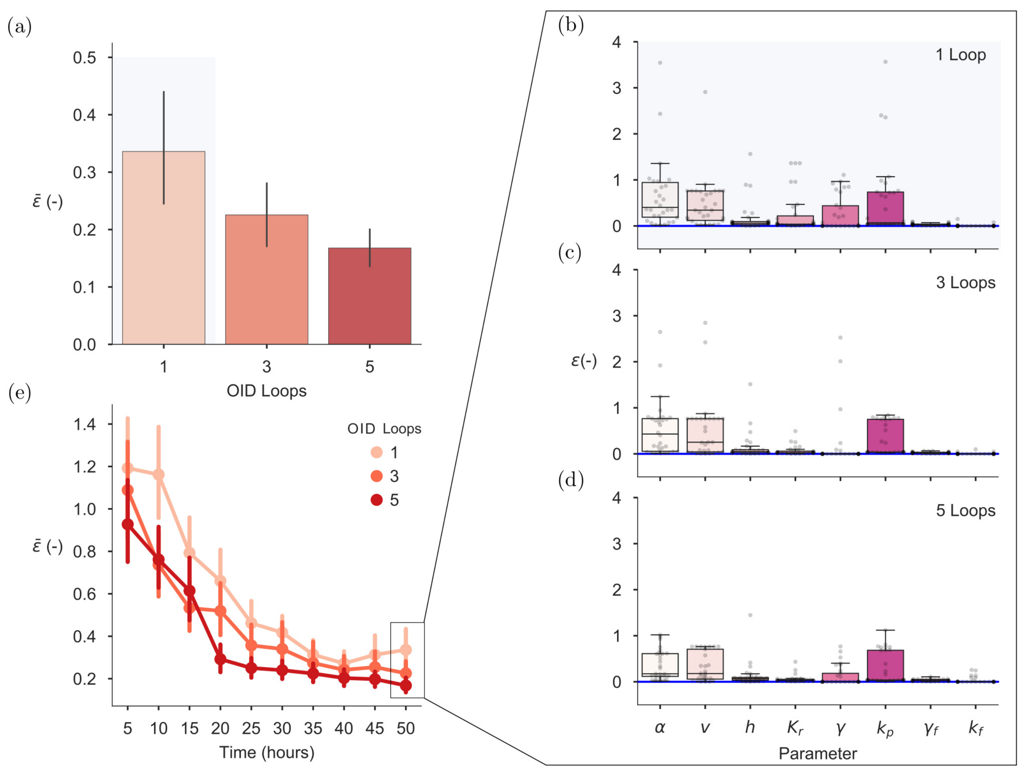
2.6. On-Line OID Supports the Automation of Model Calibration

We have shown that off-line OED can be used to reliably infer mathematical models. Nevertheless, the necessary intervention of human experts at each identification cycle [8] could increase the cost and weaken the robustness of model calibration. To address this problem, we propose to automate model inference through integrating PE/OED and in vivo experiments in an on-line, closed loop. In off-line model identification (Figure 6a), PE/OED is performed before and after the experiment; in on-line model identification, the experiment consists of a sequence of n sub-experiments or loops. In each sub-experiment i, once the waiting time for updating the model ($t_s$) has elapsed, parameter estimates are refined using the measured data, and MBOED on the current model, $\mathcal{M}\left(p_i\right)$, is used to compute the optimal input, $u_{i+1}$, for the next loop (Figure 6b).

We explore the dependency of parameter uncertainty on the trade-off between the duration of the sub-experiments and number of OID loops for n equal to 1 (off-line), 3 and 5 (on-line) using $N_j=30$ input profiles. The results show that the average relative error, $\overline{\epsilon }$, after 50 h of experiment is a decreasing function of the number of loops. Specifically, $n=5$ enables a 54% reduction in $\overline{\epsilon }$ over off-line optimally designed inputs (Figure 7a) because of the improvement in accuracy of the estimates of poorly identifiable parameters ($\alpha$ and $\gamma$) (Figure 7b–d). Finally, the evaluation of $\overline{\epsilon }$ every 5 h reveals that on-line OID accelerates the convergence of the average relative error: when $n=5$, 20 h of experiment would provide parameter estimates with an higher accuracy than those inferred over 50 h of off-line OID (Figure 7e).

3. Discussion

Ensuring the accurate and efficient inference of mathematical models represents a route to their widespread use in synthetic biology. In this paper, the quantification of the informative content of different input classes encourages the integration of MBOED in the characterisation pipeline of biological parts. We reached this conclusion by identifying a deterministic model for the orthogonal, inducible promoter designed by Gnügge et al. [10]. We chose to consider a regulated promoter as, in eukaryotes, each node in a synthetic network requires a new promoter. Furthermore, it is generally assumed that the low complexity of synthetic promoters makes the definition of informative, intuitive, experimental schemes amenable. Clearly, our results challenge this belief (Figure 4f).

Aiming to compare the informativeness of the different input classes, we recovered the model structure ($M_{PLac}$) proposed in [10]. The noticed gap between the simulated and experimental transition-region of the dose–response curve prompted us to attempt refining the calibration of $M_{PLac}$. We cast model inference as a multi-experiment fitting problem and address it using cross-validation. Despite finding that $M_{PLac,r}$ gives a 56% improvement in the fitting over $M_{PLac}$ (Figure 2c), we can only speculate on the cause of this enhancement.

We next verified that the dynamics of $M_{PLac,r}$, described by pseudo-data generated using this model, could be exhaustively captured by the lower-order model $M_{IP,r}$ (Figure 3). This result and the smaller computational cost incurred in MBOED with a simpler model led us to select $M_{IP,r}$ as a reference model of the underlying biological system in the subsequent analysis.

We found that experiments with optimised inputs improve model calibration when compared to intuition-driven inputs (Figure 4f). Interestingly, we could not recover the instinctive difference between the performances of the intuition-driven classes of inputs (Figure 4f). In addition, it is important to note that the lower average error yielded by the optimised inputs does not imply that all parameter estimates improve. For example, pulse inputs allow a narrower $\epsilon$ distribution for $k_p$ to be attained (Figure 4b–d). Nevertheless, optimally designed inputs support the decrease in the variability of the estimates of poorly identifiable parameters, e.g., $\alpha$ and $\gamma$ (Figure 4b–d). We further explored the properties of the optimised input profiles, seeking for features to which the higher accuracy of parameter inference could be ascribed. The cluster analysis by self-organising maps revealed the presence of five groups with differential performance (Figure 5a). Here, the clusters providing smaller average relative error ($\overline{\epsilon }$) were denoted by high induction levels at the fourth step. It is worth considering that, despite the system being initialised in absence of induction, the optimiser selected low IPTG concentrations at the beginning of the experiment: an observation which highlights the relevance of MBOED.

Finally, we investigated the improvement of on-line over off-line OID as a first step towards the automation of model calibration. Indeed, on-line OID would promote a standardised, more robust, and cost-effective identification of mathematical models. We found that on-line OID further improves the calibration of poorly identifiable parameters (Figure 6b–d), leading to a monotonic increase in the accuracy of parameter estimates with the number of loops (Figure 6a), although we expect this increase to eventually stop. In fact, once the experiment duration has been defined, the performance of on-line OID depends on the properties $t_H$, the duration of the sub-experiments, and $t_S$, the waiting time for updating the model. $t_H$ represents a trade-off between the number and duration of each loop; $t_S$ between the amount of data acquired in each iteration and the computational cost of PE/OED. Notably, the faster convergence of the estimates to the true parameter value observed with on-line OID would allow the overall duration of the experiment to be reduced.

Overall, these results suggest that the model-based design of dynamic perturbations would underpin our ability to perform a painstaking inference of mathematical models of biological systems: a requirement if synthetic biology is to advance as an enabling technology founded on engineering principles.

4. Methods

4.1. Generating Pseudo Experimental Data for the Identification of $M_{IP,r}$

To re-calibrate parameter values in $M_{IP}$ and obtain $M_{IP,r}$, we chose to simulate the response of $M_{PLac,r}$ to step, pulse, ramp and random inputs over 3000-min long experiments. For each of these four input classes, we defined a generating function; we then designed three inputs for each class. Step inputs are obtained using:

$$u_{\mathrm{step}}\left(t\right)=\left\{\begin{array}{cc}a,\hfill & \mathrm{if}c\le \left(t\mathrm{mod}2c\right)<2c\hfill \\ b,\hfill & \mathrm{if}0\le \left(t\mathrm{mod}2c\right)<c\hfill \end{array}\right.$$

where a, b and c were set to $\left(5\mathsf{\mu }\mathrm{M},0\mathsf{\mu }\mathrm{M},250\min \right)$, respectively, for the first of the three time-profiles (Figure 3a); $\left(10\mathsf{\mu }\mathrm{M},0\mathsf{\mu }\mathrm{M},500\min \right)$ for the second; and $\left(1000\mathsf{\mu }\mathrm{M},10\mathsf{\mu }\mathrm{M},500\min \right)$ for the third.

To obtain pulse inputs, we used the following definition:

$$u_{\mathrm{pulse}}\left(t\right)=\left\{\begin{array}{cc}a,\hfill & \mathrm{if}50\min \le \left(t\mathrm{mod}60\min \right)<60\min \hfill \\ b,\hfill & \mathrm{if}0\min \le \left(t\mathrm{mod}60\min \right)<50\min \hfill \end{array}\right.$$

where a, b were set to $\left(10\mathsf{\mu }\mathrm{M},5\mathsf{\mu }\mathrm{M}\right)$ for the first time-profilef $\left(100\mathsf{\mu }\mathrm{M},10\mathsf{\mu }\mathrm{M}\right)$ for the second input (Figure 3b–f) and $\left(1000\mathsf{\mu }\mathrm{M},600\mathsf{\mu }\mathrm{M}\right)$ for the third.

As generating function of the ramp input, we used:

$$u_{\mathrm{ramp}}\left(t\right)=\left\{\begin{array}{cc}\frac{at}{1500},\hfill & \mathrm{if}0\min \le t<1500\min \hfill \\ a-\frac{at}{1500},\hfill & \mathrm{otherwise}\hfill \end{array}\right.$$

where a was set to 10 $\mathsf{\mu }$M, 100 $\mathsf{\mu }$M (Figure 3c) and 1000 $\mathsf{\mu }$M for each of the three inputs generated for this class. It should also be noted that a Zero Order Holder filter with a window of 60, 150 and 250 min was applied to the first, second and third inputs, respectively.

Finally, the pseudo-random inputs are defined as:

$$u_{\mathrm{random}}\left(t\right)=\left\{\begin{array}{cc}a,\hfill & \mathrm{if}0\min \le \left(t\mathrm{mod}c\right)<c\hfill \end{array}\right.$$

where a and c were set to $\left(\mathcal{U}(0\mathsf{\mu }\mathrm{M},10\mathsf{\mu }\mathrm{M}),60\min \right)$ for the first time-profile (Figure 3d), $\left(\mathcal{U};(0\mathsf{\mu }\mathrm{M},90\mathsf{\mu }\mathrm{M}),150\min \right)$ for the second; and $\left(\mathcal{U}(0\mathsf{\mu }\mathrm{M},900\mathsf{\mu }\mathrm{M}),250\min \right)$ for the third.

In all simulations, we added a 5% Gaussian noise and assigned the initial conditions of the system to the steady state values derived from a 24 h simulation of $M_{PLac,r}$ with 0 $\mathsf{\mu }$M IPTG as the input. All experiments were simulated in AMIGO2 [9] and Citrine was sampled every 5 min. For more details on these procedures, we refer the reader to our GitHub repository [17].

4.2. Generating Pseudo Experimental Data for the Comparison of Input Classes

The inputs we used to compare the informative content of different stimuli were defined as follows:

$$u_{\mathrm{step}}\left(t\right)=\left\{\begin{array}{cc}a,\hfill & \mathrm{if}0\min \le \left(t\mathrm{mod}200\right)<100\min \hfill \\ b,\hfill & \mathrm{if}100\min \le \left(t\mathrm{mod}200\right)<200\min \hfill \end{array}\right.$$

where, for each of the $N_j$ inputs, a and b are two random values extracted from $\mathcal{U}(0\mathsf{\mu }\mathrm{M},1000\mathsf{\mu }\mathrm{M})$.

$$u_{\mathrm{pulse}}\left(t\right)=\left\{\begin{array}{cc}0,\hfill & \mathrm{if}10\min \le \left(t\mathrm{mod}60\min \right)<60\min \hfill \\ a,\hfill & 0\min \le \left(t\mathrm{mod}60\min \right)<10\min \hfill \end{array}\right.$$

where a is drawn from $\mathcal{U}(0\mathsf{\mu }\mathrm{M},1000\mathsf{\mu }\mathrm{M})$.

$$u_{\mathrm{random}}\left(t\right)=\left\{\begin{array}{cc}a,\hfill & \mathrm{if}0\min \le \left(t\mathrm{mod}80\min \right)<80\min \hfill \end{array}\right.$$

where a is drawn from $\mathcal{U}(0\mathsf{\mu }\mathrm{M},1000\mathsf{\mu }\mathrm{M})$.

In all simulations, we added a 5% Gaussian noise and set the initial conditions of the system to the analytical steady-state of $M_{IP,r}$ with IPTG equal to 0 $\mathsf{\mu }$M; all experiments were simulated in AMIGO2 [9] and Citrine was sampled every 5 min. For more details on these procedures we refer the reader to our GitHub repository here [17].

4.3. Parameter Estimation

Parameter estimation was formulated as a non-linear optimisation problem, whose objective is to identify the parameter values that minimise a scalar measure of the distance between model predictions and (pseudo) experimental data. We used the weighted least squares as a cost function, with weights set to the inverse of the experimental noise. This is defined as Gaussian noise with variance equal to 5% of the maximum value reached by the output, simulated with the true parameter values $p^{*}$, within an experiment. To solve the optimisation problem, we relied on eSS [11]: a hybrid method that combines a global and a local search to speed up convergence to optimal solutions. In the initial phase, eSS explored the space of solutions, and then, as local search, we employed the nonlinear least squares solver.

To strengthen the predictive capabilities of the calibrated models, we used cross-validation in the identification of $M_{PLac,r}$ and $M_{IP,r}$. In both cases, the available experimental datasets were randomised and split into training (66%) and test (33%) sets. Parameter estimation was run on the training set starting from 100 initial guesses for the parameter vector. The latter were obtained as Latin hypercube samples within the allowed boundaries for the parameters. Among the optimal solutions, the one that minimises the SSE on the test set was selected as the vector of parameter estimates. We note that, when comparing the informative content of different input classes, parameter estimation was not performed using cross-validation. Details on the allowed bounds for the parameters and the scripts used for parameter estimation are provided in the GitHub repository [17].

4.4. Off-Line Optimal Experimental Design

To reflect wet-lab experimental constraints, under the hypothesis of using a microfluidic-based platform, we fixed the sampling times (1 every 5 min) and the experiment duration (3000 min). We further set the initial condition to the steady-state in absence of induction. As a result, we restricted the optimisation to identifying the input (IPTG) time profile that maximises the information yield of the experiment. Here, information was quantified as a metric defined on the Fisher Information Matrix ($\mathcal{F}$) [6,13], whose formulation for the homoscedastic case reads:

$$\mathcal{F}=\sum _{i=1}^N\frac{1}{{\sigma }^2}{\left[{\nabla }_{p}y\left(i\right)\right]}^T\left[{\nabla }_{p}y\left(i\right)\right]$$

(3)

where $y\left(i\right)$ is the value of the observable (Citrine), simulated with the parameter vector p, at the ith sampling instant, ${\sigma }^2$ represents its variance and N is the number of sampling times. Note that ${\sigma }^2$ are independently distributed samples drawn from a normal distribution with mean 0 and variance equal to the 5% of the maximum expression level of Citrine.

The $\mathcal{F}$ sets a lower bound on the variance of the parameter estimates through the Cramer–Rao inequality:

$$\mathcal{C}\ge {\mathcal{F}}^{-1}$$

(4)

where $\mathcal{C}$ is the covariance matrix. Intuitively, as the eigenvalues of the $\mathcal{F}$ are related to the inverse of parametric variances, attempting to maximise the determinant of $\mathcal{F}$ (D-optimality) corresponds to minimising the product of the parametric variances.

To find the most informative input ($u^{*}$), we formulated MBOED as an optimal control problem and searched for:

$$u^{*}=\underset{u}{argmax}\left|\mathcal{F}\left(M_{IP,r}(p^{*},u)\right)\right|$$

(5)

where $p^{*}$ is the parameter vector considered for OID. We note that, in each of the $N_j=100$ designed input profiles, the optimisation started from an initial guess for the parameter vector $p^{*}$ obtained as Latin hypercube sample within the allowed boundaries for the parameters. Based on a comparison between Differential Evolution ($DE$) [18], a global optimisation method featuring good convergence properties and suitable for parallelisation, and eSS [11] (results not shown), we selected the latter to solve the optimisation problem. The solvers fminsearch and fmincon were employed for the local and final-local search. Details on the allowed bounds for the parameters, the 100 initial guesses for the parameter vector and the true value of the parameters are provided in the GitHub repository [17].

4.5. Clustering of the Optimised Inputs

To further explore the properties of the optimally-designed inputs, we performed a cluster analysis by self-organising maps (SOM). This is a two-stage approach, in which the $N_j$ = 100 optimally designed inputs are grouped into a reduced number of prototype vectors by the SOM, and then the SOM is clustered. In the first phase, the SOM was linearly initialised as a 7 × 7 rectangular lattice which was trained for 30 iterations in batch mode, using a Gaussian neighbourhood function with constant radius equal to 1 [15]. Linear initialisation and batch training algorithm were selected for their computational efficiency [19]. The remaining parameters, upon exploration of alternative sizes, neighbourhood functions and initial/final radii, were identified as the configuration with the best quantitative measure of mapping quality, i.e., quantization and topological errors. Hence, the SOM nodes were grouped by hierarchical, agglomerative clustering using Euclidean distance (default) and average linkage. The obtained dendrogram was verified for dissimilarity and inconsistency.

Abstraction of the inputs to the prototype vectors was performed using the SOM Toolbox [15]. We used the Statistical and Machine learning MATLAB toolbox to cluster the SOM. Principal component analysis of the prototype vectors was performed in Python.

4.6. On-Line Optimal Experimental Design

To compare the performance of on-line OID with the off-line counterpart, we adopted the same sampling times (1 every 5 min), experiment duration (3000 min) and number of steps (15). This resulted in $t_H=$ 1000 and 600 min for n = 3 and 5 loops, respectively. We further set the initial condition of each experiment to the steady-state in absence of induction. In each sub-experiment, the optimal input was applied to the system to simulate Citrine dynamics and to obtain pseudo-data. The augmented dataset was used to update the model parameters and compute the initial state of the next sub-experiment. Hence, MBOED was used to design the input for the following loop. We note that, to reduce the computational cost incurred in on-line OID, the $\mathcal{F}$ was calculated only over the sampling times of each loop.

5. Conclusions and Future Work

In summary, we highlight MBOED as an enabling tool for the inference of predictive mathematical models of biological parts in synthetic biology. Focusing on the identification of a mathematical model of a synthetic promoter, whose simplicity would encourage the definition of intuitive experimental schemes, our computational results report a ∼60% increase in the confidence of parameter estimates when optimally designed input profiles are compared to intuition-driven stimuli. While this result confirms evidence in the scientific literature [7], in this work, we highlight for the first time, to the best of our knowledge, that the reduction of the parameter search space allowed by on-line OED further leads to an 84% improvement in the accuracy of parameter inference. Besides the necessary in vivo validation and investigation of the scalability of computational cost for systems of higher complexity, these results motivate efforts towards the development of cyber physical platforms to automate model calibration, in which MBOED and microfluidic experiments are embedded in an identification loop.

References

1. Cameron, D.E.; Bashor, C.J.; Collins, J.J. A brief history of synthetic biology. Nat. Rev. Microbiol. 2014, 12, 381–390. [Google Scholar] [CrossRef] [PubMed]
2. Ellis, T.; Wang, X.; Collins, J.J. Diversity-based, model-guided construction of synthetic gene networks with predicted functions. Nat. Biotechnol. 2009, 27, 465–471. [Google Scholar] [CrossRef] [PubMed] [Green Version]
3. Nielsen, A.A.; Der, B.S.; Shin, J.; Vaidyanathan, P.; Paralanov, V.; Strychalski, E.A.; Ross, D.; Densmore, D.; Voigt, C.A. Genetic circuit design automation. Science 2016, 352, aac7341. [Google Scholar] [CrossRef] [PubMed]
4. Salis, H.M. The ribosome binding site calculator. In Methods in Enzymology; Elsevier: Amsterdam, The Netherlands, 2011; Volume 498, pp. 19–42. [Google Scholar]
5. Borkowski, O.; Ceroni, F.; Stan, G.B.; Ellis, T. Overloaded and stressed: Whole-cell considerations for bacterial synthetic biology. Curr. Opin. Microbiol. 2016, 33, 123–130. [Google Scholar] [CrossRef] [PubMed]
6. Ljung, L. System Identification: Theory for the User, Ptr Prentice Hall Information and System Sciences Series; Prentice Hall: Upper Saddle River, NJ, USA, 1999. [Google Scholar]
7. Bandara, S.; Schlöder, J.P.; Eils, R.; Bock, H.G.; Meyer, T. Optimal experimental design for parameter estimation of a cell signaling model. PLoS Comput. Biol. 2009, 5, e1000558. [Google Scholar] [CrossRef] [PubMed]
8. Ruess, J.; Parise, F.; Milias-Argeitis, A.; Khammash, M.; Lygeros, J. Iterative experiment design guides the characterization of a light-inducible gene expression circuit. Proc. Natl. Acad. Sci. USA 2015, 112, 8148–8153. [Google Scholar] [CrossRef] [PubMed] [Green Version]
9. Balsa-Canto, E.; Henriques, D.; Gábor, A.; Banga, J.R. AMIGO2, a toolbox for dynamic modeling, optimization and control in systems biology. Bioinformatics 2016, 32, 3357–3359. [Google Scholar] [CrossRef] [PubMed] [Green Version]
10. Gnugge, R.; Dharmarajan, L.; Lang, M.; Stelling, J. An Orthogonal Permease–Inducer–Repressor Feedback Loop Shows Bistability. ACS Synth. Biol. 2016, 5, 1098–1107. [Google Scholar] [CrossRef] [PubMed]
11. Egea, J.A.; Balsa-Canto, E.; García, M.S.G.; Banga, J.R. Dynamic Optimization of Nonlinear Processes with an Enhanced Scatter Search Method. Ind. Eng. Chem. Res. 2009, 48, 4388–4401. [Google Scholar] [CrossRef]
12. Balsa-Canto, E.; Alonso, A.A.; Banga, J.R. Computational procedures for optimal experimental design in biological systems. IET Syst. Biol. 2008, 2, 163–172. [Google Scholar] [CrossRef] [PubMed]
13. Walter, E.; Pronzato, L. Identification of Parametric Models from Experimental Data; Springer: Berlin, Germany, 1997. [Google Scholar]
14. Kohonen, T.; Maps, S.O. Springer series in information sciences. Self-Organ. Maps 1995, 30, 105–176. [Google Scholar]
15. Vesanto, J.; Himberg, J.; Alhoniemi, E.; Parhankangas, J.; Parhankangas, J. Self-organizing map in Matlab: The SOM Toolbox. In Proceedings of the Matlab DSP Conference, Espoo, Finland, 16–17 November 1999; Volume 99, pp. 35–40. [Google Scholar]
16. Liu, Y.; Li, Z.; Xiong, H.; Gao, X.; Wu, J. Understanding of internal clustering validation measures. In Proceedings of the 2010 IEEE 10th International Conference on Data Mining (ICDM), Sydney, Australia, 13–17 December 2010; pp. 911–916. [Google Scholar]
17. Available online: https://github.com/csynbiosysIBioEUoE/ODidiPAmCSB2018SI (accessed on 29 June 2018).
18. Storn, R.; Price, K. Differential evolution—A simple and efficient heuristic for global optimization over continuous spaces. J. Glob. Optim. 1997, 11, 341–359. [Google Scholar] [CrossRef]
19. Liu, Y.; Weisberg, R.H.; Mooers, C.N. Performance evaluation of the self-organizing map for feature extraction. J. Geophys. Res. Oceans 2006, 111. [Google Scholar] [CrossRef] [Green Version]
20. Available online: https://datasync.ed.ac.uk/index.php/s/xGL4oSbJMyu91Bt (accessed on 29 June 2018).
Figure 1. The inducible promoter constructed by Gnügge et al. [10]. The ( t e t O ) 2 and the ( l a c O ) 2 operator sequences were cloned upstream and downstream of the TATA box of a native S. cerevisiae promoter. The assembly was genomically integrated in a budding yeast strain constitutively expressing the heterologous transcription factors, tetracycline responsive transactivator (tTA) and LacI repressor, and the lactose permease (Lac12). The expression of the Citrine fluorescent reporter is used as a faithful readout of the promoter activity, induced by the non-metabolizable chemical isopropyl β D 1 thiogalactopyranoside (IPTG).
Processes 06 00148 g001
Figure 2. Ability of the M P L a c , M P L a c , r and M I P model structures to recapitulate the experimental data. (a) Dose–response curve after 24 h of induction with the reported IPTG concentrations. Experimental data, median (filled squares) and inter-quartile range (errorbars) of Citrine distributions were retrieved from [10]. In-silico dose–response curve for M P L a c (grey), M P L a c , r (cyan) and M I P (purple) are shown as solid lines. (b) For each induction level, the dynamics of Citrine was sampled at five equidistant time points. This is showcased for IPTG = 5 μ M . (c) Barplot of the sum of squared errors of predictions (SSE), quantifying the predicted deviations from empirical data.
Processes 06 00148 g002
Figure 3. Pseudo-experiments for the calibration of M I P , r . Step (a); pulse (b); ramp (c); and random (d) inputs (red line) were used to simulate Citrine dynamics in M P L a c , r . By sampling the simulated expression profiles and adding 5% Gaussian noise, we obtain pseudo-data (green circles). The green line represents the response of the calibrated M I P , r to these data.
Processes 06 00148 g003
Figure 4. Analysis of the informative content of different input classes for model parameterisation. (a) An example of an optimally designed input (red line) applied to M I P , r to simulate Citrine dynamics (green circles). The response of the calibrated model to the input is shown as a green solid line. Box plots, overlaid with swarmplots, of the relative error ( ε ) of parameter estimates for: step (b); pulse (c); random (d); and optimised (e) inputs. (f) Bar plot of the average relative error ( ε ¯ ) computed for each input class.
Processes 06 00148 g004
Figure 5. Clustering of the optimised inputs. (a) Bar chart of the average relative error for the inputs associated to each cluster. (b) Parallel plot of the prototype vectors of each cluster. The average of the nodes grouped in a cluster is shown as a continuous line. The shaded area reports on the maximum and minimum IPTG value at each step. (c) Scatter plot and two-sigma error ellipses of the principal component analysis of the prototype vectors.
Processes 06 00148 g005
Figure 6. Comparison of off-line and on-line OID for model identification. (a) In off-line OID, the current model M ( p 0 ) is used to design the optimal input (red line) to be applied to the cells in an experiment of duration t H . At the end of the experiment, Citrine expression data (green circles) inform the refinement of the model to give M ( p 1 ) . (b) In on-line OID, the experiment is structured as a sequence of n sub-experiments (e.g., n = 2 ), each lasting t H . Before the experiment begins, M ( p 0 ) is used to optimally design the input, u 1 , to be applied in the first sub-experiment. After a time t S , the model is refined to M ( p 1 ) and used to design the input, u 2 , for sub-experiment 2. The procedure is iterated for the duration of the experiment.
Processes 06 00148 g006
Figure 7. Improvement of off-line over on-line OID for model calibration. (a) Bar plot of the average relative error, ε ¯ , obtained with n = 1 (off-line OID and highlighted with a shadowed patch), and n = 3 and n = 5 OID loops after 50 h of experiment. Box plots overlaid with swarmplots of the relative error, ε , of parameter estimates for off-line (b) and on-line OID with 3 (c) and 5 (d) loops. We limit the maximum of the y-axis to simplify the comparison of the relative errors. (e) ε ¯ as a function of time for the three cases.
Processes 06 00148 g007