An Analysis of Uncertainty Propagation Methods Applied to Breakage Population Balance

Abstract

In data-driven empirical or hybrid modeling, the experimental data influences the model parameters and thus also the model predictions. The experimental data has some variability due to measurement noise and due to the intrinsic stochastic nature of certain pharmaceutical processes such as aggregation or breakage. To use predictive models, it is imperative that the accuracy of the predictions is known. To this extent, various uncertainty propagation techniques applied to a predictive breakage population balance model are studied. Three uncertainty propagation techniques are studied: linearization, sigma point, and polynomial chaos. These are compared to the uncertainty obtained from Monte Carlo simulations. Linearization performs the worst in the given scenario, while sigma point and polynomial chaos methods have similar performance in terms of accuracy.

1. Introduction

In the pharmaceutical industry, mathematical models are an integral part of the quality by design (QbD) paradigm [1,2,3]. Mathematical models may be white-box (mechanistic), black-box (empirical), or gray-box (hybrid). White-box models are based on a mechanistic understanding of the underlying physical, chemical phenomena that are well understood (e.g., the Arrhenius equation). Black-box models are data-driven models that do not consider any physics behind an operation and are valid only in a very specific region of operation. Gray-box models combine both a theoretical understanding and empirical data. As complete mechanistic models can be very expensive to build, most models used in the industry fall in the empirical or hybrid categories.

Inevitably, the experimental data used to build such a model affects the estimated values of the model parameters and hence the model predictions. A modeler must thus carefully design the experiment such that the information content in the data is maximized to obtain the most accurate parameter estimates [4]. However, even with well designed and accurate experiments, some variability is inherent to the modeling process. This variability arises from a lack of measurement samples (both number and repetitions), the noise that corrupts measurements, and the intrinsic stochastic nature of certain processes such as breakage or aggregation [5]. Uncertainty refers to the precision of the parameters estimated from given data. In many cases, this uncertainty is described by the confidence interval of the parameter estimate. If decisions must be made using models with uncertain parameters, it is important that how uncertainty affects model prediction is known.

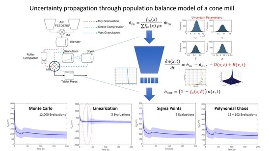
This work describes how the accuracy of a model prediction can be described from the confidence intervals of the estimated parameters. The focus lies on model of conical screen mill developed by Barasso et al. [6]. The conical screen mill is a popular size reduction equipment used to delump blended active pharmaceutical ingredients (APIs), break tablets for recovery, or deliver a specific reduced particle size. A classical way of modeling milling equipment is by using the population balance framework [7]. Under the assumption of well-mixedness, population balance models (PBMs) are hybrid models which can describe the temporal change in the particle number density in a physical volume through

$$\frac{\partial n(t,\mathbf{x})}{\partial t}+\frac{\partial }{\partial \mathbf{x}}\left(n(t,\mathbf{x})\frac{d\mathbf{x}}{dt}\right)=\mathcal{B}(t,\mathbf{x})-\mathcal{D}(t,\mathbf{x})$$

(1)

with initial condition

$$n(0,\mathbf{x})=n^{\mathrm{in}}\left(\mathbf{x}\right).$$

(2)

$n(t,\mathit{x})$ describes the particle number density as a function of time, t, and the internal state vector, $\mathbf{x}$. The internal state vector defines the properties which are used to describe the number densities in the distribution, e.g., concentration, porosity, and particle size. The second term in the equation describes the continuous change over the internal state vector arising from processes such as crystal growth, consolidation, or evaporation. Processes involving the appearance or disappearance of particles at discrete points in the internal state vector (e.g., aggregation or breakage) are not taken into account by this term but by the birth and death terms on the right-hand side: $\mathcal{B}(t,\mathbf{x})$ and $\mathcal{D}(t,\mathbf{x})$, respectively. In many cases, a one-dimensional (1D) PBM is formulated using only the particle size (x) as the internal state vector. However, multidimensional PBMs considering properties such as concentration or porosity can easily be formulated to account for complex situations that can arise. In case of a pure breakage process, such as the conical screen mill, the above equation can be reduced to a one-dimensional PBM as

$$\frac{\partial n(t,x)}{\partial t}=\underset{\mathcal{B}(t,x)}{\underbrace{{\int }_x^{\infty }b(x,y)S\left(y\right)n(t,y)dy}}-\underset{\mathcal{D}(t,x)}{\underbrace{\phantom{{\int }_x^{\infty }}S(x)n(t,x)}}.$$

(3)

The term $\mathcal{B}(t,x)$ on the right-hand side of the equation represents the birth of the particle by the breakage process. The breakage function $b(x,y)$ is the probability function describing the formation of particles with size x by the breakage of the particles with size y. The selection function $S\left(x\right)$ describes the rate of breakage of particles with size x. The term $\mathcal{D}(t,x)$ on the right describes the death of the particle because of breakage. The selection function and the breakage distribution function are normally empirical functions whose parameters need to be estimated from a given experimental dataset.

In this work, the cone mill model developed in [6] is used as a predictive model. The uncertainty in the parameters is propagated to the median particle size $\left(d_{50}\right)$. The $d_{50}$ is a common size indicator used in the pharmaceutical industry to describe the size of an API. In many cases, design decisions are based on the $d_{50}$, making it a critical quality attribute (CQA). As such, it is important that the accuracy of the $d_{50}$ value predicted from the model is known. In the pharmaceutical industry, the most common method used is the Monte Carlo method. This method works well for relatively simple models which are not computationally expensive. However, for complex expensive models, Monte Carlo quickly becomes unattractive due to the computational time required. The aim of this work is to present other methods that can be used to propagate uncertainty through a nonlinear model, without requiring excessive sampling as in the Monte Carlo method. Three uncertainty propagation techniques are considered for comparison: linearization, sigma points, and polynomial chaos expansion (PCE). As no analytical steady state solution is available for the PBM, these methods will be evaluated against the Monte Carlo method. In case the analytical solution is available, the accuracy of the techniques could be compared using an error norm (e.g., [8]). All four methods are described in detail in Section 2.1. The cone mill model and its parameters are described in Section 2.2. The numerical method used to solve the PBM is briefly described in Section 2.3. This study will not discuss or compare the various discretization schemes available to solve the PBMs numerically.

2. Materials and Methods

2.1. Uncertainty Propagation Methods

In this section, the four uncertainty propagation techniques are described. For brevity and ease, a dynamic model is represented in its general form

$$\dot{\mathbf{x}}=f(\mathbf{x},\theta )$$

(4)

$$\mathbf{y}=h\left(\mathbf{x}\right(\theta \left)\right)$$

(5)

where $\mathit{x}\in {\mathbb{R}}^{n_x}$ is the state vector, $\mathbf{y}\in {\mathbb{R}}^{n_y}$ is the output vector, and $\theta \in {\mathbb{R}}^{n_{\theta }}$ is the uncertain parameter vector.

2.1.1. Monte Carlo Method

In the Monte Carlo method, a large number of pseudo-random input parameters are drawn from the estimated parameter distribution [9]. Based on these parameters, the model output is calculated, and the mean and the confidence interval is determined empirically through the law of large numbers. The Monte Carlo method is relatively easy to apply as there is a large availability of random number generators available. Moreover, as no assumption is made on the distributions, this method can be considered the most accurate. However, there is no general guidance on the number of parameters that should be drawn to obtain reliable results and as such tens of thousands of model simulations may be required, making it computationally very expensive.

2.1.2. Linearization

The linearization approach uses a linear approximation of the variance-covariance matrix of the model output. This approximation is obtained from a first-order Taylor series expansion of the model with respect to the uncertain parameter. However, the higher-order terms in the expansion can only be neglected if the uncertainty is smaller compared to the model curvature. If $\mathrm{S}=\partial f/\partial \theta$ is the sensitivity matrix of the model output with respect to the uncertain parameters, and $V_{\theta }$ is the variance-covariance matrix of the parameters, the variance-covariance matrix of the model output is given by

$${\mathrm{V}}_y=\mathrm{S}{\mathrm{V}}_{\theta }{\mathrm{S}}^{\top }.$$

(6)

From the variance-covariance matrix, the (1 − $\alpha$)100% confidence can be found akin to the confidence bound on parameter estimates giving [10]

$$y_{i,\mathrm{lin}}=y_i\pm t_{\left(1-\frac{\alpha }{2},n_m-n_p\right)}\sqrt{{\mathrm{V}}_y(i,i)}.$$

(7)

However, as the variance on the estimated parameter is only the lower bound on its true variance [11], the actual uncertainty on the model output can be even higher.

2.1.3. The Sigma Point Method

The sigma point method (SP) is a sampling-based method for nonlinear transformation of Gaussian random variables [12]. The parameter distribution is represented by a finite number of deterministically chosen sampling points called the sigma points. For n uncertain parameters, a set of $2n$ sigma points is chosen as

$$\sigma \leftarrow \sqrt{(n+\kappa ){\mathrm{V}}_{\theta }}$$

(8)

$${\theta }_{\sigma }={\theta }_0\pm \sigma .$$

(9)

A set of model outputs can be calculated from the sigma points as

$${\mathbf{y}}_0=h\left(\mathbf{x}\left({\theta }_0\right)\right)$$

(10)

$${\mathbf{y}}_{\sigma }=h\left(\mathbf{x}\left({\theta }_{\sigma }\right)\right).$$

(11)

The mean can then be calculated as

$${\overline{\mathbf{y}}}_{\mathrm{sig}}=\frac{1}{n+\kappa }\left[\kappa {\mathbf{y}}_0+\frac{1}{2}\sum ^{2n}{\mathbf{y}}_{\sigma }\right],$$

(12)

while the variance-covariance matrix is calculated as

$${\mathbf{V}}_y=\frac{1}{n+\kappa }\left[\kappa ({\mathbf{y}}_0-{\overline{\mathbf{y}}}_{\mathrm{sig}}){({\mathbf{y}}_0-{\overline{\mathbf{y}}}_{\mathrm{sig}})}^{\top }+\frac{1}{2}\sum ^{2n}({\mathbf{y}}_{\sigma }-{\overline{\mathbf{y}}}_{\mathrm{sig}}){({\mathbf{y}}_{\sigma }-{\overline{\mathbf{y}}}_{\mathrm{sig}})}^{\top }\right].$$

(13)

The uncertainty on the model output can the be predicted using Equation (7). When no information on output distribution is available, it is suggested that the value of $\kappa$ be set to $3-n$. This ensures that the root mean squared error in the mean prediction is minimized up to the fourth order [12]. In the sigma point approach, the model equations need to be solved $2n+1$ times.

2.1.4. The Polynomial Chaos Method

In the polynomial chaos expansion method (PCE), the model response is approximated by an infinite series of orthogonal basis functions [13]. For practical applications, the infinite series is truncated to a limited number of terms M.

$$y_{\mathrm{PCE}}=\sum _{i=0}^M{a}_i{\mathsf{\Phi }}_i\left(\theta \right).$$

(14)

The basis function can be estimated using the Wiener–Askey scheme [14], which suggests the use of various orthogonal polynomials based on the probability distribution of the parameters. The number of terms in the series is determined by the number of uncertain parameters (n) and the order of the polynomials (m) used as

$$M+1=\frac{(n+m)!}{n!m!}.$$

(15)

Once the PCE has been formulated, the mean and the variance of the model output can be approximated from the PCE coefficients as

$${\overline{\mathbf{y}}}_{\mathrm{PCE}}=a_0$$

(16)

$${\mathbf{V}}_y=\sum _{i=1}^M{a}_i^2.$$

(17)

Different methods exist to determine the coefficients of the PCE. Intrusive methods use Galerkin projection to compute the coefficients [15,16]. These methods can be a complex set of equations that need to be derived and solved for each case. Non-intrusive methods are based on sampling by repeated model evaluations at the collocation points [13,17]. The number of collocation points should be higher or equal to the number of coefficients in the PCE. The non-intrusive approach is used in this study.

2.2. The Mathematical Model for the Cone Mill

The cone mill consists of a rotating impeller that provides impact energy to the particles. The particles stay in the mill until they are reduced to a size smaller than the screen aperture. Different types of impeller shapes are available, along with a variety of screens with different shapes and a variety of aperture sizes. The screen size is the most significant parameter affecting the particle size of the milled product [18,19]. Even then, the impeller speed, impeller shape, and the screen size have a statistically significant impact on the final size distribution [20]. For the same impeller shape, either an increase in impeller speed or a decrease in screen size leads to a lower mean particle size.

In this work, the model developed by Barasso et al. [6] is utilized. The model describes the evolution of the number of particles over time with respect to the particle size represented by its volume. The model considers a cone mill operated in a starve feed mode, which is common for continuous operations.

$$\frac{dn(x,t)}{dt}={\dot{n}}_{in}(x,t)-{\dot{n}}_{out}(x,t)-\mathcal{D}(u,t)+\mathcal{B}(u,t).$$

(18)

Here, $n(x,t)$ is the number of particles of volume x in the mill at any time t. This model is a simple extension of the batch breakage equation described in Equation (3) to a continuous system by including the feed inlet (${\dot{n}}_{in}(x,t)$) and the product outlet (${\dot{n}}_{out}(x,t)$).

${\dot{n}}_{in}(x,t)$, the number of particles being fed to the mill, is calculated from the mass flow rate $\left({\dot{m}}_{in}\right)$ as

$${\dot{n}}_{in}(x,t)=\frac{f_{in}\left(x\right)}{\sum f_{in}\left(x\right)}\frac{{\dot{m}}_{in}}{\rho x},$$

(19)

with $\rho$ being the density of the particles, and $f_{in}\left(x\right)$ being the volume-weighted distribution of the feed particles. ${\dot{n}}_{out}(x,t)$ is the outlet flow based the following screen classification model.

$${\dot{n}}_{out}(x,t)=\left({\dot{n}}_{in}(x,t)-\mathcal{D}(x,t)+\mathcal{B}(x,t)\right)\left(1-f_d\left(x\right)\right)$$

(20)

$$f_d\left(x\right)=\{\begin{array}{ll}0& ,\mathrm{if}d\left(x\right)\le (1-\delta )d_{screen}\\ \frac{d\left(x\right)-(1-\delta )d_{screen}}{\delta d_{screen}}& ,\mathrm{if}(1-\delta )d_{screen}<d\left(x\right)\le d_{screen}\\ 1& ,\mathrm{if}d\left(x\right)>d_{screen}\end{array}$$

(21)

where $d\left(x\right)$ is the particle diameter associated with volume x. $d_{screen}$ is the screen opening, and $\delta$ is a parameter which determines the critical diameter. A particle with diameter larger than the screen opening will be retained in the mill, whereas a particle smaller than the critical diameter will exit the mill. The screen is non-ideal for particle diameters between the screen opening and the critical diameter.

The terms $\mathcal{B}(x,t)$ and $\mathcal{D}(x,t)$ describe the birth and death of the particle of size x by breakage as described in Equation (3).

The breakage rate depends on the particle and process parameters and is represented as

$$S\left(x\right)=\alpha v_{imp}{\left(\frac{x}{x_{ref}}\right)}^{\gamma }$$

(22)

with $\alpha$ and $\gamma$ as model parameters that need to be tuned, and $v_{imp}$ is the impeller speed of the cone mill shaft. The breakage distribution function is chosen to be a log-normal function

$$b(x,y)=\frac{C\left(y\right)}{x\sigma }exp\left[-\frac{{\left(logx-log\frac{y}{n}\right)}^2}{2{\sigma }^2}\right].$$

(23)

The volume of the parent particle is represented by y, and $C\left(y\right)$ is chosen to fulfill the mass conservation constraint

$${\int }_0^{y}xb(x,y)dx=y.$$

(24)

The parameter values and the operating conditions for the model are given in

Table 1. Parameters and operating parameters for the cone mill adapted from [6].

Parameter	Value	Standard Deviation
Critical screen size parameter, $\delta$	$0.44$	$0.07$
Selection function parameter, $\alpha$	$8.82\times {10}^{-6}$	$1.01\times {10}^{-6}$
Selection function parameter, $\gamma$	$0.34$	$0.08$
Breakage distribution parameter, $\sigma$	$2.10$	$0.12$
Inlet mass flow, ${\dot{m}}_{\mathrm{in}}$	$7.4$ g/s	-
Particle density, $\rho$	$0.74$ g/cc	-
Inlet distribution median, ${\mu }_{\mathrm{in}}$	$4.81\times {10}^{-5}{\mathrm{m}}^3$	-
Inlet distribution deviation, ${\sigma }_{\mathrm{in}}$	$0.25$	-
Volume of first cell, $x_1$	$6.54\times {10}^{-17}{\mathrm{m}}^3$	-
Selection reference volume, $x_{ref}$	$2.23\times {10}^{-9}{\mathrm{m}}^3$	-
Breakage distribution function parameter, n	$2.68\times {10}^5$	-
Impeller speed, $v_{imp}$	4923 RPM	-
Impeller speed, $v_{imp}$ after 30 s	1500 RPM	-
Screen aperture, $d_{screen}$	$1575\mathsf{\mu }\mathrm{m}$	-

. The parameter estimates and their confidence bounds computed by Barasso et al. [6] from the experimental data are used in this study.

2.3. The Numerical Method

As the analytical solution of the PBM described in Section 2.2 is impossible, the PBM must be solved numerically. A variety of other methods based on size grid discretization are available in the literature [7,21,22,23,24]. The fixed pivot technique (FPT) of Kumar and Ramakrishna [21] is used in this study. The general idea behind the FPT is to discretize the size range into small sections and to represent each section by a pivot. If a new particle is born at a size other than that of the pivot, it is divided between the neighboring pivots such that any two integral properties are conserved.

The continuous size domain is first discretized into I cells of size $\Delta x_i=x_{i-1/2}-x_{i+1/2}$, $i=1,\dots ,I$. Every individual cell $[x_{i-1/2},x_{i+1/2}]$ is represented by a size $x_i$. The particle distributions are considered to be point masses at these points. Thus, the entire size distribution can be represented by

$$N_i\left(t\right)={\int }_{x_{i-1/2}}^{x_{i+1/2}}n(x,t)dx.$$

(25)

The equation for the FPT by conserving the number and mass are given as follows:

$$\frac{d{N}_i}{dt}=\sum _{j\ge i}^I{\eta }_{i,j}{S}_j{N}_j-S_i{N}_i$$

(26)

where

$${\eta }_{i,j}={\int }_{x_i}^{x_{i+1}}\frac{x_{i+1}-x}{x_{i+1}-x_i}b(x,x_j)dx+{\int }_{x_{i-1}}^x\frac{x-x_{i+1}}{x_i-x_{i-1}}b(x,x_j)dx.$$

(27)

3. Results

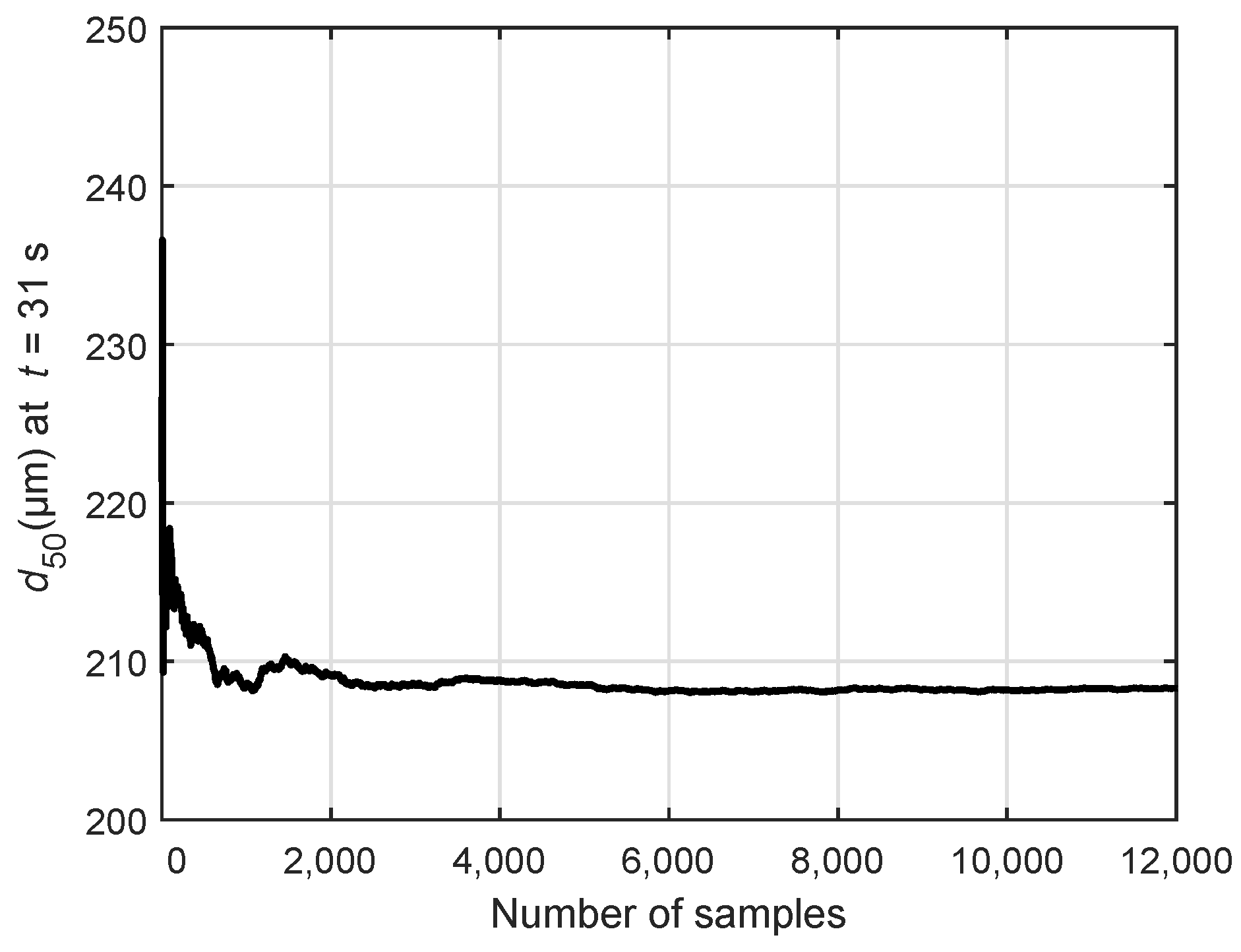
Four parameters-critical screen parameter $\delta$, the two selection function parameters $\alpha \mathrm{and}\gamma$, and breakage distribution parameter $\sigma$, are considered uncertain for this study. These parameters are assumed to be Gaussian random variables, with the mean as the nominal value and the standard deviation described in Table 1.

The model is used to predict the $d_{50}$ of the API exiting the mill. The mill is operated with a 1575 $\mathsf{\mu }$m sieve and an impeller speed of 4923 RPM. After $30\mathrm{s}$ of operation, the impeller speed is changed to 1500 RPM. This is done to highlight the benefits and drawbacks of the various methods considered here. All the computations are carried out in MATLAB 2017b (The MathWorks Inc., Natick, MA, USA). The PBM is solved by discretizing the model using the fixed pivot technique described in Section 2.3. The discretization leads to a system of differential algebraic equations, which was solved using a variable order numerical difference formula (ode15s function). Normally, the choice of discretization also affects the solution. In this study, only the fixed pivot method with 100 grid points is considered. A comparison of various discretization schemes for the cone mill is provided in [25].

All the methods will be compared at time just after the impeller speed is changed. This region represents the maximum dynamic change in the model and, as such, can be used to critically evaluate the methods. As the set point change is induced after 30 s, the evaluation is carried out on the $d_{50}$ value at 31 s. The uncertainty bands in all cases refer to the 95% confidence intervals calculated based on the F-distribution.

3.1. The Monte Carlo Method

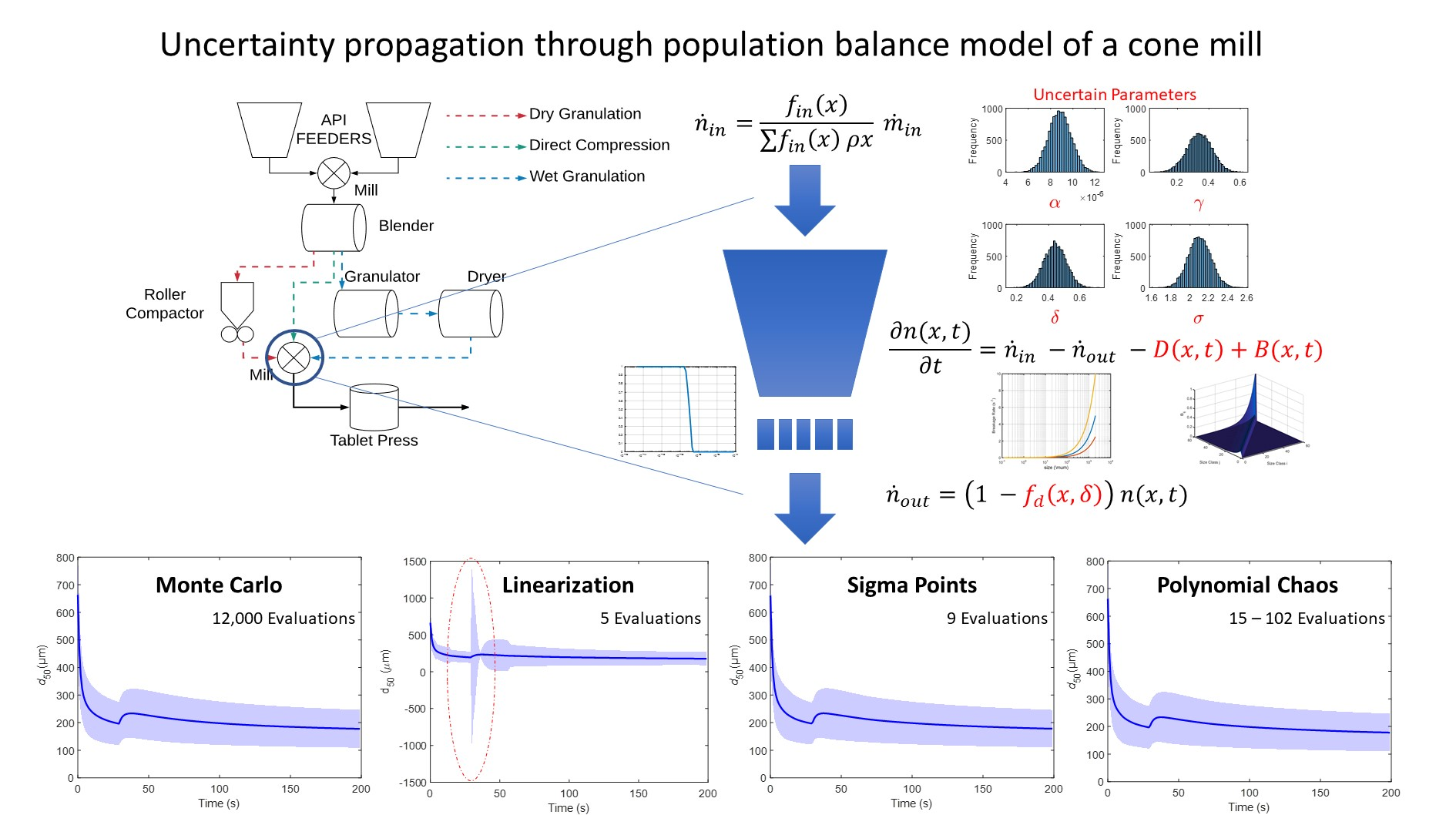
The Monte Carlo variance decays as $1/\sqrt{N}$, with N being the number of samples. Thus, if a large number of samples are used, the Monte Carlo method can be considered the most accurate. However, the results of the Monte Carlo depend on the number of samples that are drawn from the given distribution. Some studies discuss the methods for determining the number of iterations required in the Monte Carlo method. However, these calculations are not always feasible in practice. Thus, the appropriate number of iterations must be determined empirically. Figure 1 illustrates the mean value of the $d_{50}$ for a different number of samples. It can be seen that the mean value stabilizes above 4000 samples. Thus, at least 5000 samples should be used to obtain reliable information from the Monte Carlo simulations. 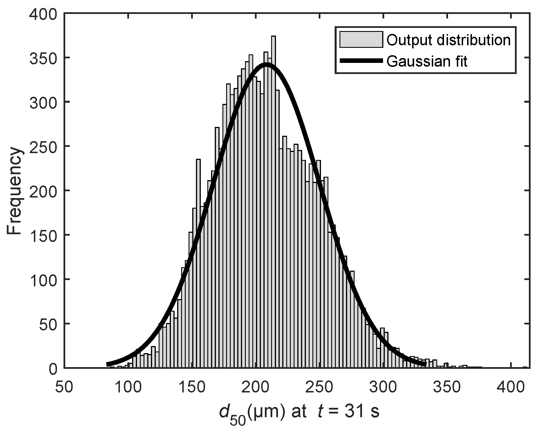For further comparison, 12,000 samples are drawn from a normal distribution as depicted in Figure 2. The $d_{50}$ distribution at 31 s is depicted in Figure 3. This output is tested for normality using the Kolmogrov–Smirnov (KS) test. It should be noted that, even after 12,000 model evaluations, the KS test rejects the hypothesis that the output could be drawn from a normal distribution. Thus, more samples would be required to evaluate the true variance of the distribution. For this study, the distribution is fit to a normal curve. 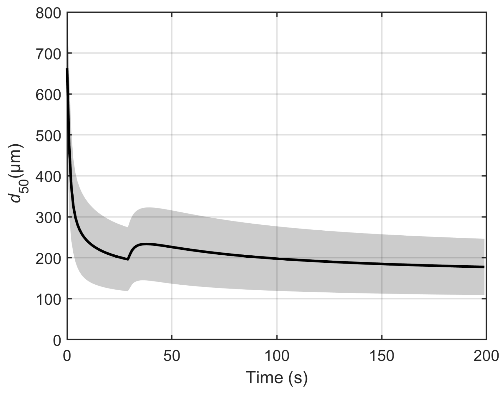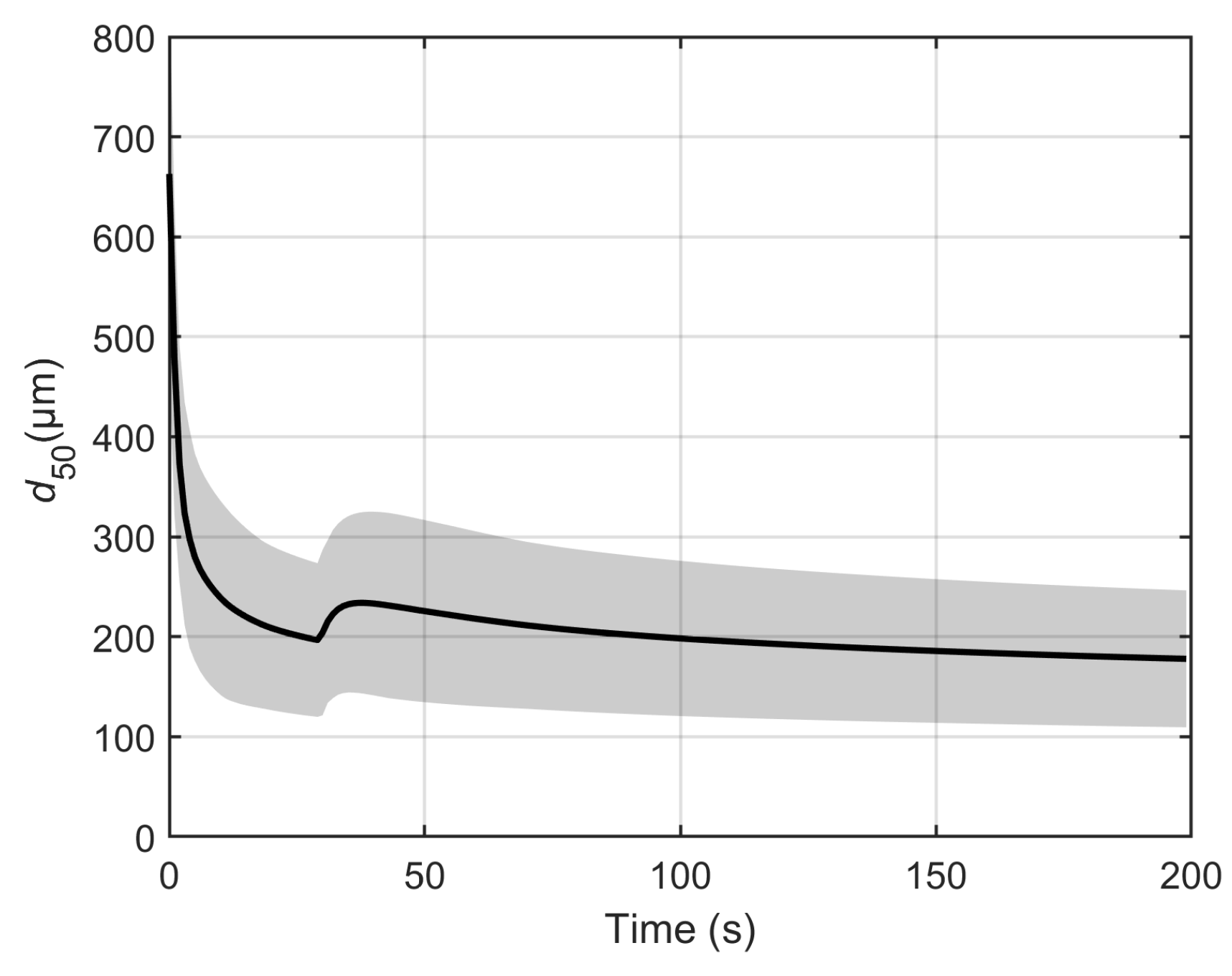It is observed that, for the $d_{50}$ value at 31 s, the distribution fit has a mean of 208.366 ± 0.741 $\mathsf{\mu }$m and a standard deviation of 41.7409 ± 0.5177 $\mathsf{\mu }$m. This fit is considered good enough to use 12,000 Monte Carlo samples to quantify the uncertainty. The result of the Monte Carlo simulation over the entire time is shown in Figure 4.

As such, the three other methods will be compared to the solution from the Monte Carlo method.

3.2. Linearization Method

The main advantage of the linearization method is its ease of implementation and relatively low computational burden. The Jacobian matrix required can be calculated numerically. In this study, a simple finite difference scheme is used to calculate the Jacobian.

$$J_i=\frac{\partial \mathbf{y}}{\partial {\theta }_i}\approx \frac{h\left(x\left({\theta }_i\right)\right)-h\left(x({\theta }_i-\Delta \theta )\right)}{\Delta \theta }.$$

(28)

The deviation $\Delta \theta$ was chosen to be ${10}^{-3}$ times the nominal parameter value. Thus, for the current system, with four uncertain parameters, the linearization method is required to evaluate the model five times to determine the Jacobian.

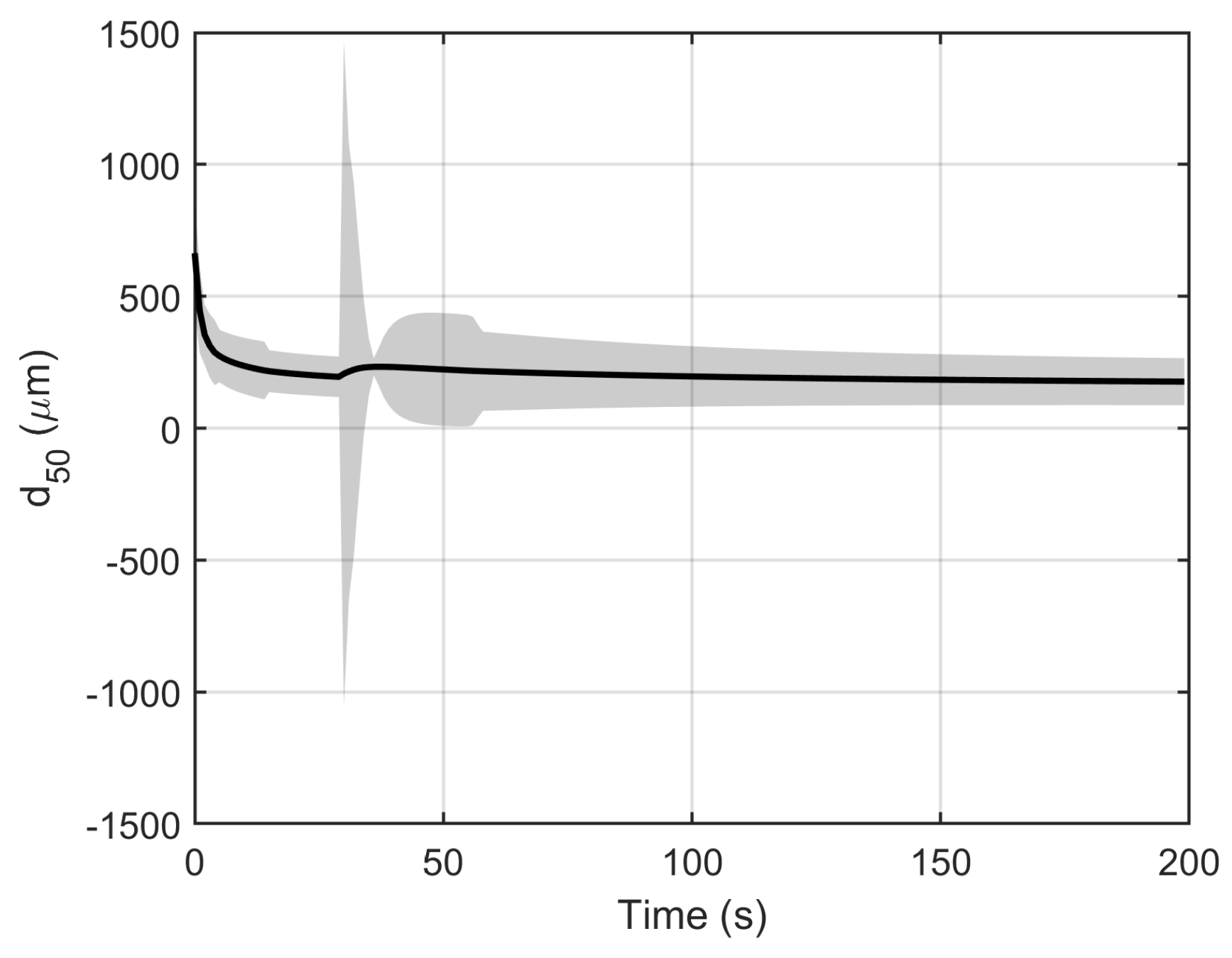
The result of the linearization method is depicted in Figure 5. It can be observed that, in some regions of operation (after 100 s), the linearization method yields a good approximation of the uncertainty. However, it overpredicts the uncertainty in regions of high system dynamics. As the evaluation of Jacobian is extremely sensitive to model curvature, linearization completely fails in regions of high model dynamics. This is evident from Figure 5. At the moment the setpoint change is induced (30 s), linearization grossly overpredicts the uncertainty associated with model prediction. Thus, linearization should be used with caution, especially when there are dynamic conditions to which the model is sensitive.

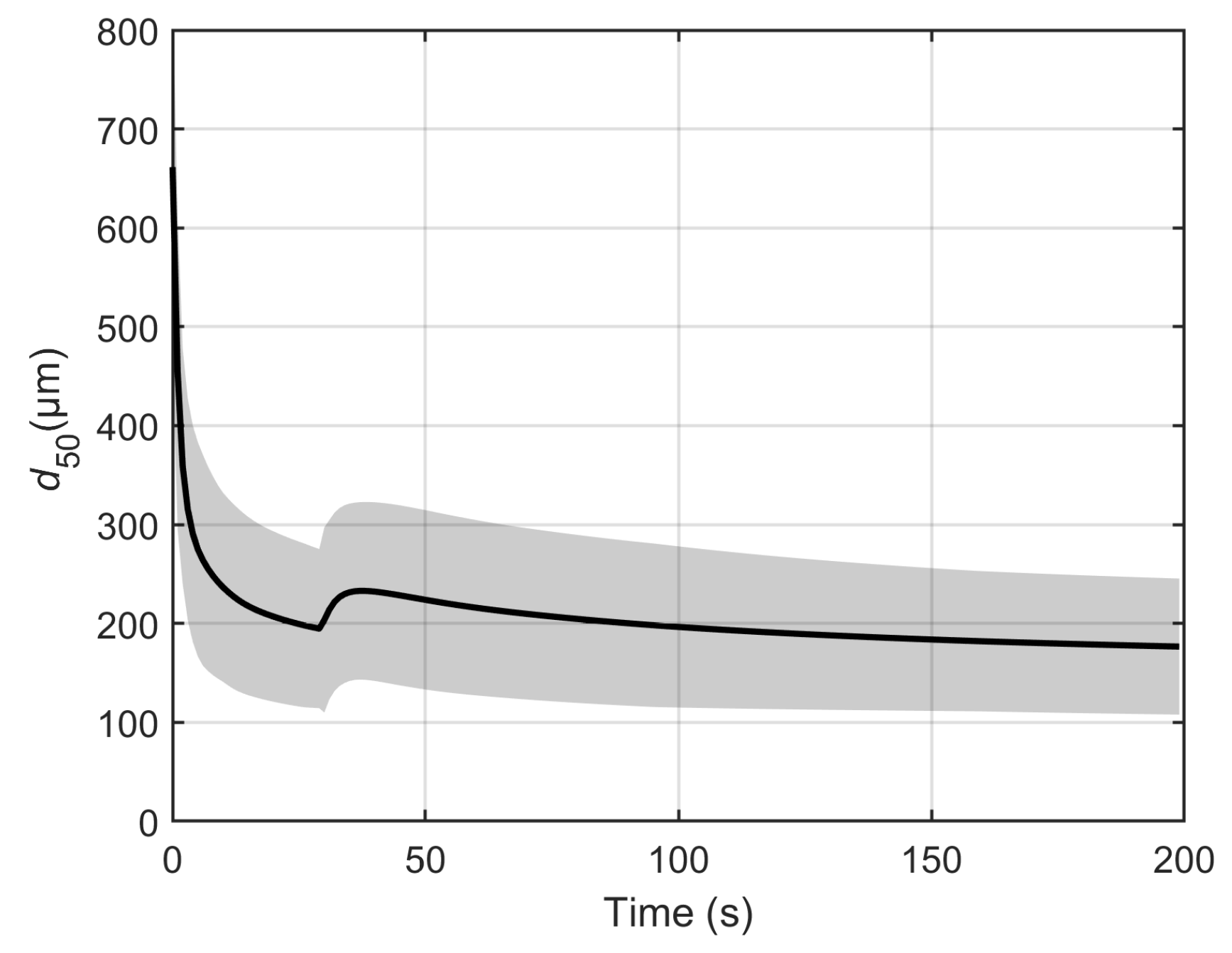
3.3. Sigma Point Method

With four uncertain parameters, nine sigma points need to be calculated, and the model is evaluated at these sampling points. As can be observed from Figure 6, the results of the sigma point method closely mimic the Monte Carlo simulations even in the region of the setpoint change.

This shows that the sigma point approach is more reliable than the linearization approach. The performance comes at a cost, as more function evaluations are required. However, the number of iterations is still orders of magnitude smaller than that for the Monte Carlo method. The major drawback of the sigma point method is that it requires the parameters to be normally distributed.

3.4. Polynomial Chaos Expansion

As the parameters in this study are assumed to be normally distributed, Hermite polynomials are used based on the Weiner–Askey scheme [14]. PCEs of order 1 (PCE1) and 2 (PCE2) are studied, and the linear regression method is used to determine the coefficients of the PCEs. Based on Equation (15), PCE1 leads to 5 unknown coefficients, and PCE2 to 15 unknown coefficients. A major issue in application of PCE is sampling. To determine the coefficients, a set of K ($K\ge M+1$) samples from the random variables is sampled. Generally, $K=2(M+1)$ samples are considered to be sufficient for a robust solution. However, the choice of samples highly affects the accuracy of the results. Thus, a variety of sampling techniques are proposed in the literature [26,27]. In this study, we use sigma points from Section 3.3 augmented by a Latin-hypercube-based design [28] to sample in the feasible space denoted by the parameter confidence interval. 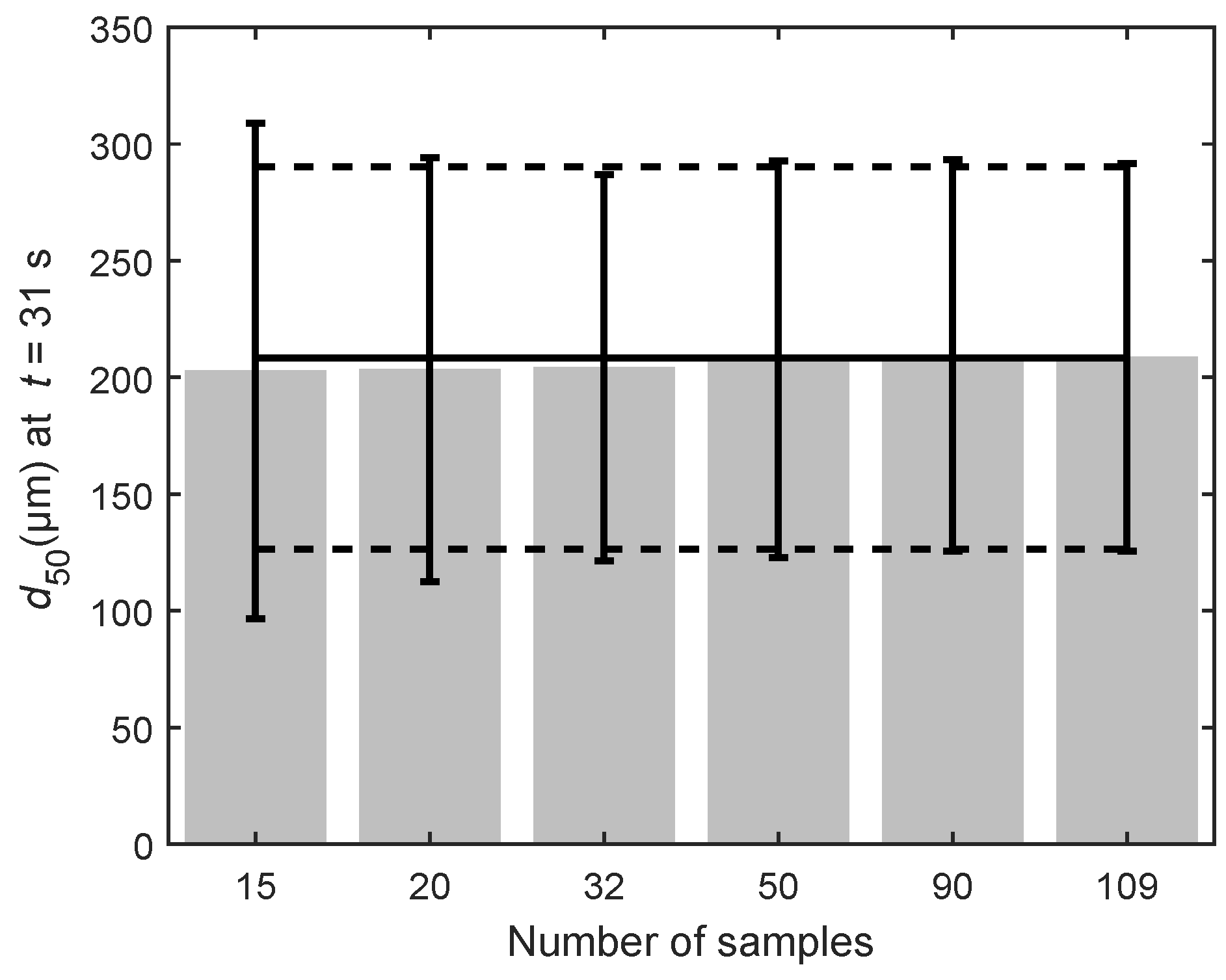The results of PCE1 (with nine sampling points chosen to be the sigma points) are depicted in Figure 7, and the results of PCE2 (with 32 sampling points) are depicted in Figure 8. In Figure 9, the accuracy of the PCE2 method is evaluated based on the number of samples used. The mean $d_{50}$ value (bars), and its variance (error bars) starts to converge towards the Monte Carlo value (solid & dashed horizontal line) with an increasing number of samples. Although not used here, PCE can easily be expanded to use third-order polynomials. However, in that case, the number of samples will increase to a minimum of 72. Generally, the increase in accuracy achieved by higher-order PCE is not enough to warrant the increased computational burden [13]. In general, we can say that PCE methods with adequate sampling approximate the mean and variance accurately.

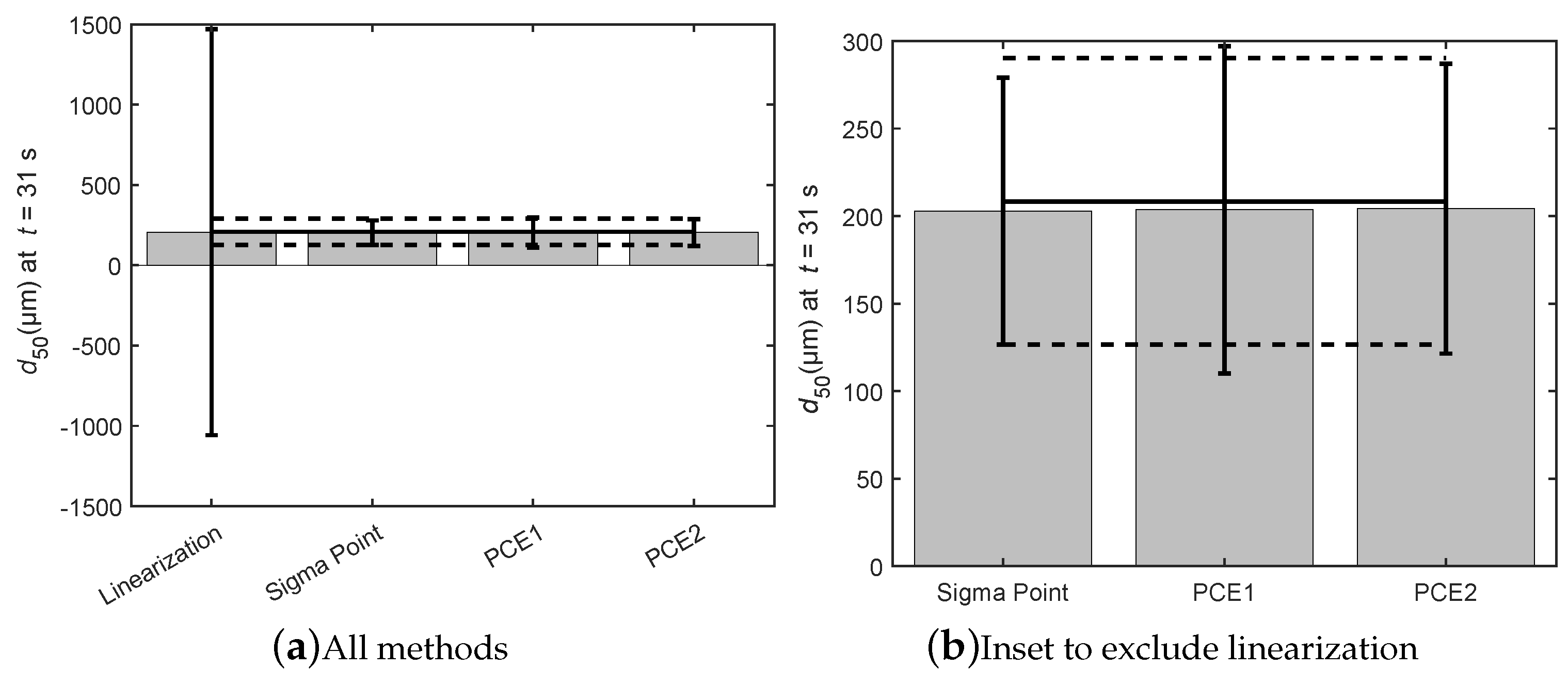
In Figure 10, the four methods are compared using the $d_{50}$ evaluated at 31 s. It is clearly seen that linearization performs the worst of all the methods. As previously mentioned, this is due to the change in model curvature induced due to step change in the impeller speed at 30 s. The other techniques—sigma point, PCE1, and PCE2—result in values that are comparable to each other. The sigma point method slightly underestimates the variance, while the PCE1 method slightly overestimates the variance. The performance of the PCE methods can be improved by using more sampling points or using a higher-order polynomial. For all practical purposes, the performance of these three methods in terms of accuracy can be considered the same. 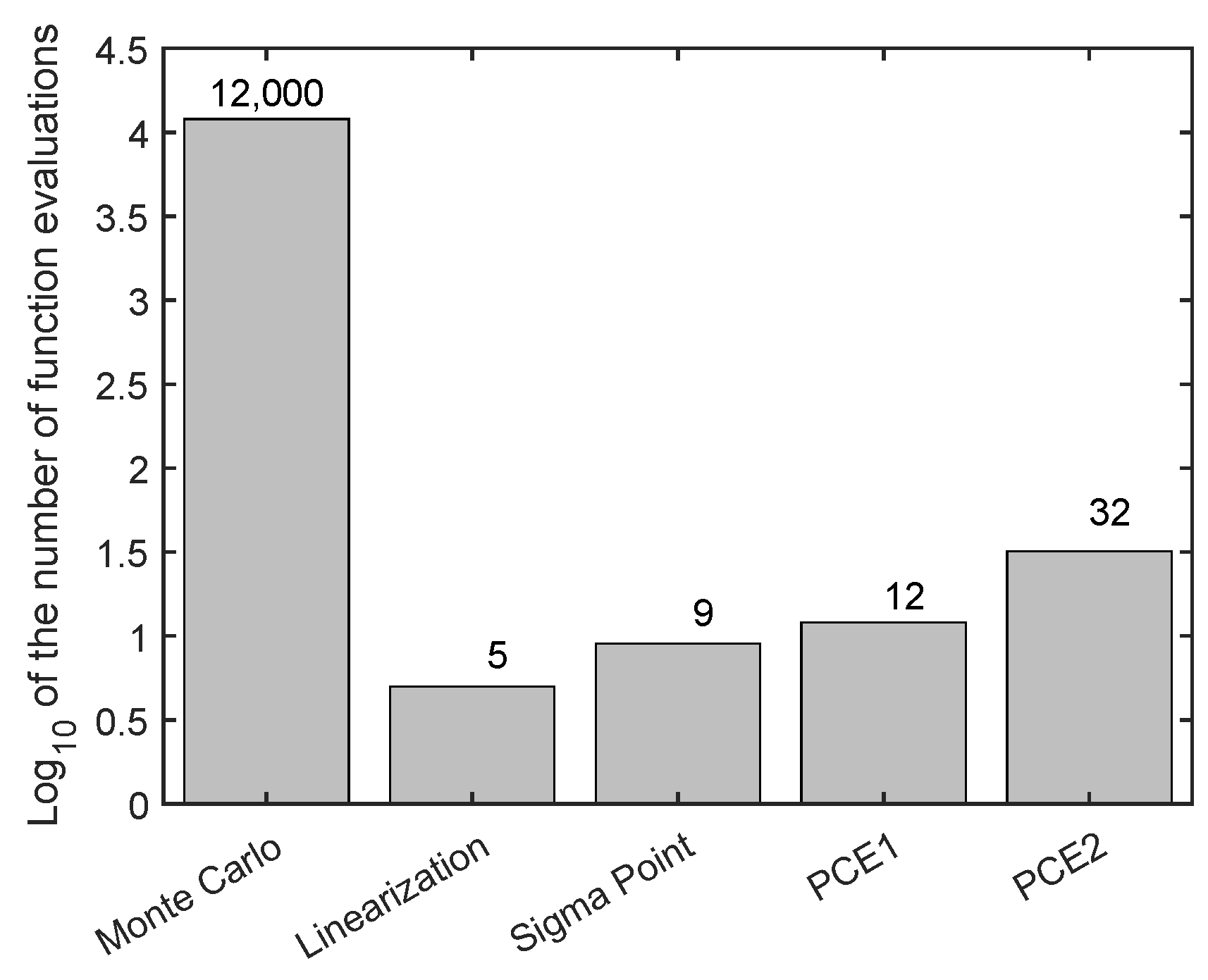Figure 11 compares the number of function evaluations required for each technique. Monte Carlo performs the worst in terms of computational time with 12,000 function evaluations. All other methods require a significantly lower number of evaluations. For the current case, SP methods seem the most suitable, as we know the parameters to be normally distributed.

4. Conclusions

Firstly, it can be concluded that the model in consideration is not adequate for any decision making, as the prediction uncertainty in terms of 95% confidence interval is high. The model needs to be improved either by using more experimental data to estimate the parameters or, if that fails, by improving the model structure.

However, the aim of the study is to discuss the selection of methods for uncertainty propagation to provide an accurate representation of the model prediction uncertainty in the breakage population balance models. The results demonstrate that, although computationally the cheapest, linearization does not provide a reliable estimate of the uncertainty. If it is known a priori that the model under consideration is smooth and not extremely nonlinear, linearization can be a good option to achieve a first estimate of the prediction uncertainty. However, in the case of highly nonlinear dynamics, other approaches are deemed necessary.

The Monte Carlo method is the most accurate way of predicting the uncertainty, but due to the difficulty in knowing the number of samples required, the method can quickly become very computationally demanding. Recently, Monte-Carlo-based methods such as multi-level Monte Carlo (MLMC) and quasi Monte Carlo (QMC) methods have gained popularity, as they reduce the computational time of the full Monte Carlo method. MLMC tries to minimize the computational time by approximating the final mean as a sum of predicted means obtained at lower accuracy (which in many cases means a lower computational time) [29]. Thus, even though MLMC leads to a larger number of function evaluations, the total computational cost could be lower than a standard Monte Carlo method. The QMC, on the other hand, relies on smart sampling strategies to reduce the number of function evaluations, thus reducing the computational time [30]. These methods, although interesting, would still lead to a fairly high computational cost and can be justified when there is no information on the distribution of uncertain parameters. However, as in the case under study, the parameters are known to be normally distributed, the other methods are more attractive.

The deterministic sampling of the model parameters in the sigma point method give it an advantage over the random sampling of the Monte Carlo method The sigma point method reduced the number of samples and function evaluations from more than 12,000 to only 9 and still provided an accurate representation of uncertainty. However, sigma point methods can only be applied when the distribution of the uncertain parameters is symmetric and unimodal.

PCE methods also lead to an extensive reduction of sampling points compared with the Monte Carlo method and provide accurate predictions on model uncertainty. PCE methods can be complex to implement. The choice of polynomials and collocation points for sampling plays an important role and, as such, is non-trivial. If the uncertain parameters are characterized by asymmetric and/or multimodal distributions, the PCE method has to be used to replace the Monte Carlo method. The choice of orthogonal polynomials depends on the distribution of the uncertain parameters and follows the Wiener–Askey scheme [14].

Thus, we can conclude by stating that the sigma point method is the most attractive method for applications such as the PBM studied here because of its ease of implementation, its accuracy in representing model uncertainty, and its computational efficiency. PCE methods become attractive when the parameter distributions are known a priori to be asymmetric or multimodal. However, when no information about parameter distributions is available, the Monte Carlo method has to be used. In such a situation, MLMC or QMC methods can reduce the computational burden.

References

1. Djuris, J.; Djuric, Z. Modeling in the quality by design environment: Regulatory requirements and recommendations for design space and control strategy appointment. Int. J. Pharm. 2017, 533, 346–356. [Google Scholar] [CrossRef] [PubMed]
2. Yu, L.X.; Amidon, G.; Khan, M.A.; Hoag, S.W.; Polli, J.; Raju, G.K.; Woodcock, J. Understanding Pharmaceutical Quality by Design. AAPS J. 2014, 16, 771–783. [Google Scholar] [CrossRef] [PubMed] [Green Version]
3. Rogers, A.J.; Hashemi, A.; Ierapetritou, M.G. Modeling of particulate processes for the continuous manufacture of solid-based pharmaceutical dosage forms. Processes 2013, 1, 67–127. [Google Scholar] [CrossRef]
4. Telen, D.; Logist, F.; Quirynen, R.; Houska, B.; Diehl, M.; Impe, J. Optimal experiment design for nonlinear dynamic (bio)chemical systems using sequential semidefinite programming. AIChE J. 2014, 60, 1728–1739. [Google Scholar] [CrossRef] [Green Version]
5. Dacey, M.; Krumbein, W. Models of breakage and selection for particle size distributions. Math. Geol. 1978, 11, 193. [Google Scholar] [CrossRef]
6. Barrasso, D.; Oka, S.; Muliadi, A.; Litster, J.D.; Wassgren, C.; Ramachandran, R. Population Balance Model Validation and Prediction of CQAs for Continuous Milling Processes: Towards QbD in Pharmaceutical Drug Product Manufacturing. J. Pharm. Innov. 2013, 8, 147–162. [Google Scholar] [CrossRef]
7. Ramakrishna, D. Population Balances; Elsevier Inc.: Amsterdam, The Netherlands, 2000. [Google Scholar]
8. Dimarco, G.; Pareschi, L.; Zanella, M. Uncertainty quantification for kinetic models in socio-economic and life sciences. In Uncertainty Quantification for Hyperbolic and Kinetic Equations; Jin, J.S., Pareschis, L., Eds.; Springer International Publishing: Cham, Switzerland, 2017; pp. 151–191. [Google Scholar]
9. Fishman, G. Monte Carlo: Concepts, Algorithms, and Applications; Springer: New York, NY, USA, 1996. [Google Scholar]
10. Seber, G.; Wild, C. Nonlinear Regression; Wiley Interscience: New York, NY, USA, 2003. [Google Scholar]
11. Walter, E.; Pronzato, L. Identification of Parmametric Models from Experimental Data; Elsevier Inc.: Amsterdam, The Netherlands, 2000. [Google Scholar]
12. Julier, S.; Uhlmann, J.K. A General Method for Approximating Nonlinear Transformations of Probability Distributions; Technical report; Robotics Research Group, Department of Engineering Science, University of Oxford: Oxford, UK, 1996. [Google Scholar]
13. Nimmegeers, P.; Telen, D.; Logist, F.; Impe, J.V. Dynamic optimization of biological networks under parametric uncertainty. BMC Syst. Biol. 2016, 10, 86. [Google Scholar] [CrossRef]
14. Xiu, D.; Karniadakis, G. The Wiener–Askey polynomial chaos for stochastic differential equations. SIAM J. Sci. Comput. 2002, 24, 619–644. [Google Scholar] [CrossRef]
15. Ghanem, R.; Spanos, P. Stochastic Finite Elements—A Spectral Approach; Springer: New York, NY, USA, 1991. [Google Scholar]
16. Debusschere, B.; Najm, H.; Pébay, P.; Knio, O.; Ghanem, R.; Maitre, O.L. Numerical challenges in the use of polynomial chaos representations for stochastic processes. SIAM J. Sci. Comput. 2004, 26, 698–719. [Google Scholar] [CrossRef]
17. Tatang, M.; Pan, W.; Prinn, R.; McRae, G. An efficient method for parametric uncertainty analysis of numerical geophysical models. J. Geophys. Res. Atmos. 1997, 102, 21925–21932. [Google Scholar] [CrossRef] [Green Version]
18. Byers, J.E.; Peck, G.E. The effect of mill variables on a granulation milling process. Drug Dev. Ind. Pharm. 1990, 16, 1761–1779. [Google Scholar] [CrossRef]
19. Verheezen, J.J.; van der Voort Maarschalk, K.; Faassen, F.; Vromans, H. Milling of agglomerates in an impact mill. Int. J. Pharm. 2004, 278, 165–172. [Google Scholar] [CrossRef] [PubMed]
20. Motzi, J.J.; Anderson, N.R. The quantitative evaluation of a granulation milling process II—Effect of ouput screen size, mill speed and impeller shape. Drug Dev. Ind. Pharm. 1984, 10, 713–728. [Google Scholar] [CrossRef]
21. Kumar, S.; Ramkrishna, D. On the solution of population balance equations by discretization I—A fixed pivot technique. Chem. Eng. Sci. 1996, 51, 1311–1332. [Google Scholar] [CrossRef]
22. Kumar, S.; Ramkrishna, D. On the solution of population balance equations by discretization II—A moving pivot technique. Chem. Eng. Sci. 1996, 51, 1333–1342. [Google Scholar] [CrossRef]
23. Kumar, J.; Warnecke, G.; Peglow, M.; Heinrich, S. Comparison of numerical methods for solving population balance equations incorporating aggregation and breakage. Powder Technol. 2009, 189, 218–229. [Google Scholar] [CrossRef]
24. Hounslow, M.J.; Ryall, R.L.; Marshall, V.R. A discretized population balance for nucleation, growth, and aggregation. AIChE J. 1988, 34, 1821–1832. [Google Scholar] [CrossRef]
25. Bhonsale, S.; Telen, D.; Van Impe, J. Comparison of numerical solution strategies for population balance models of continuous cone mill. Powder Technol. 2018. submitted for publication. [Google Scholar]
26. Zein, S.; Colson, B.; Glineur, F. An Efficient Sampling Method for Regression-Based Polynomial Chaos Expansion. Commun. Comput. Phys. 2013, 13, 1173–1188. [Google Scholar] [CrossRef]
27. Kaintura, A.; Dhaene, T.; Spina, D. Review of Polynomial Chaos-Based Methods for Uncertainty Quantification in Modern Integrated Circuits. Electronics 2018, 7, 30. [Google Scholar] [CrossRef]
28. Husslage, B.G.M.; Rennen, G.; van Dam, E.R.; den Hertog, D. Space-filling Latin hypercube designs for computer experiments. Optim. Eng. 2011, 12, 611–630. [Google Scholar] [CrossRef]
29. Giles, M. Multilevel Monte Carlo methods. Acta Numer. 2015, 24, 259–328. [Google Scholar] [CrossRef] [Green Version]
30. Dick, J.; Kuo, F.Y.; Sloan, I.H. High-dimensional integration: The quasi-Monte Carlo way. Acta Numer. 2013, 22, 133–288. [Google Scholar] [CrossRef]
Figure 1. Stability of the Monte Carlo methods with respect to the number of samples drawn. The mean value for the d 50 stabilizes after around 5000–6000 iterations.
Processes 06 00255 g001
Figure 2. Parameter distributions used for the Monte Carlo method. Twelve thousand samples are used for further comparison.
Processes 06 00255 g002
Figure 3. Distributions of d 50 value at 31 s simulated from the Monte Carlo method using 12,000 samples. The solid line shows the fit of a normal distribution to the histogram.
Processes 06 00255 g003
Figure 4. Model prediction (black solid) with 95 % confidence range (shaded) using the Monte Carlo method with 12,000 samples.
Processes 06 00255 g004
Figure 5. Model prediction (black solid) with 95 % confidence range (shaded) using the linearization method.
Processes 06 00255 g005
Figure 6. Model prediction (black solid) with 95 % confidence range (shaded) using the sigma point method.
Processes 06 00255 g006
Figure 7. Model prediction (black solid) with 95 % confidence range (shaded) using first-order polynomial chaos. Twelve samples were drawn using the Latin hypercube method.
Processes 06 00255 g007
Figure 8. Model prediction (black solid) with 95 % confidence range (shaded) using second-order polynomial chaos.
Processes 06 00255 g008
Figure 9. The number of samples used for PCE2 approximation based on the d 50 value at 31 s.
Processes 06 00255 g009
Figure 10. The different techniques with results from the Monte Carlo simulation (horizontal lines) using the d 50 value evaluated at 31 s. Figure (a) shows all four methods, while Figure (b) is an inset which excludes linearization due to its high confidence interval.
Processes 06 00255 g010
Figure 11. The number of samples or function evaluations required for each technique.
Processes 06 00255 g011