Energy Consumption and Economic Analyses of a Supercritical Water Oxidation System with Oxygen Recovery

Abstract
:1. Introduction
2. Proposal of OR for SCWO Systems
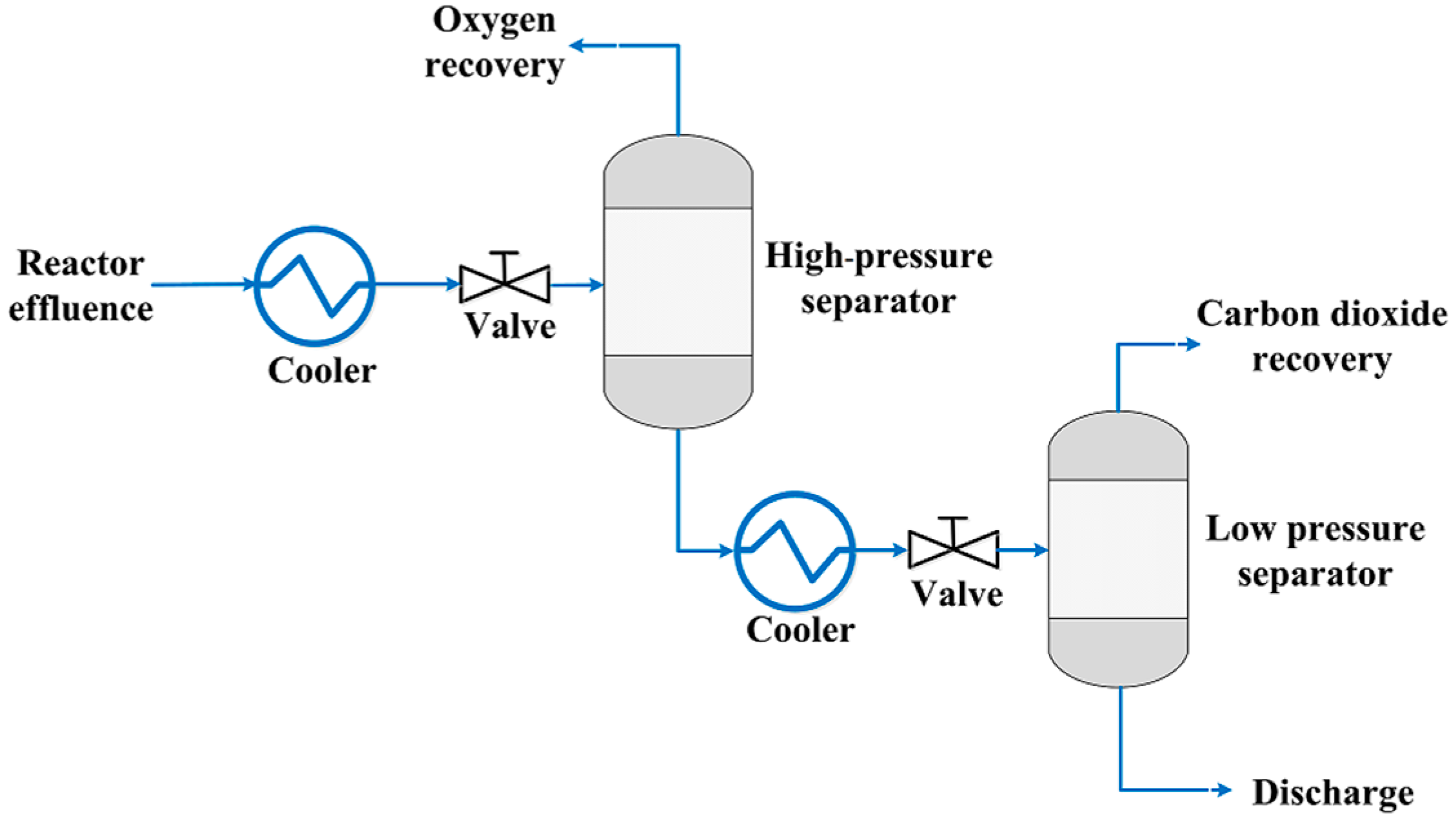
3. High-Pressure Separation for Reactor Effluent
3.1. High-Pressure Separation Process
3.2. Definition of Process Parameters
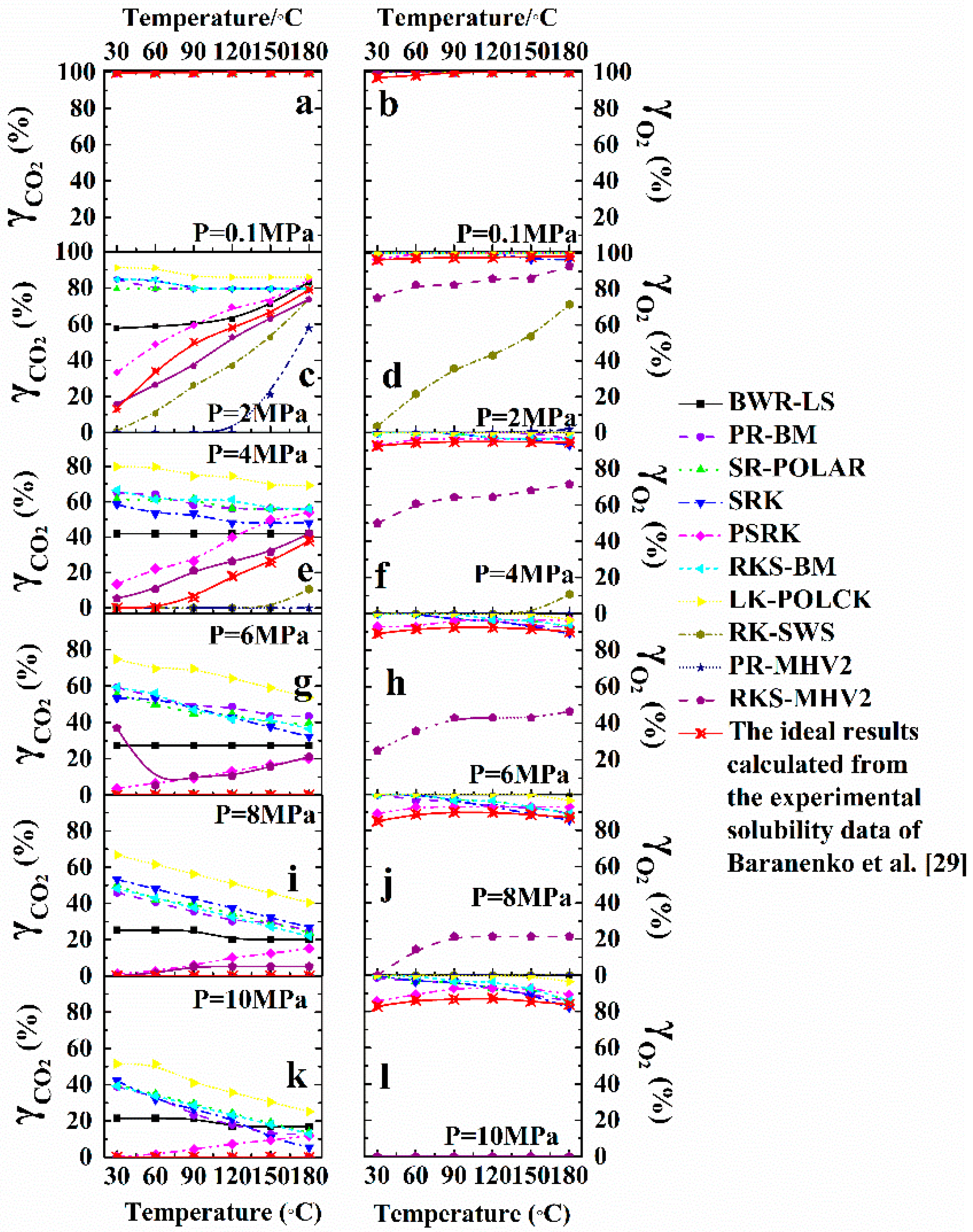
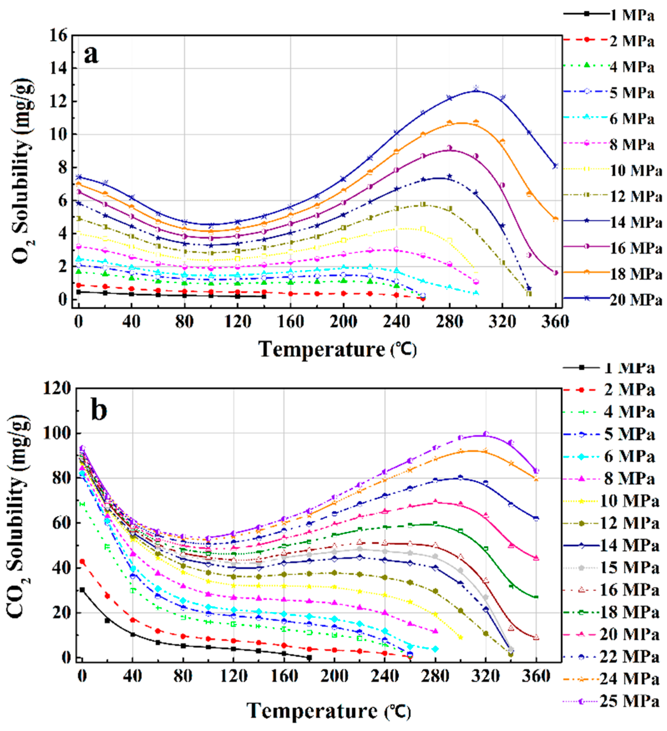
3.3. Thermodynamic Property Models
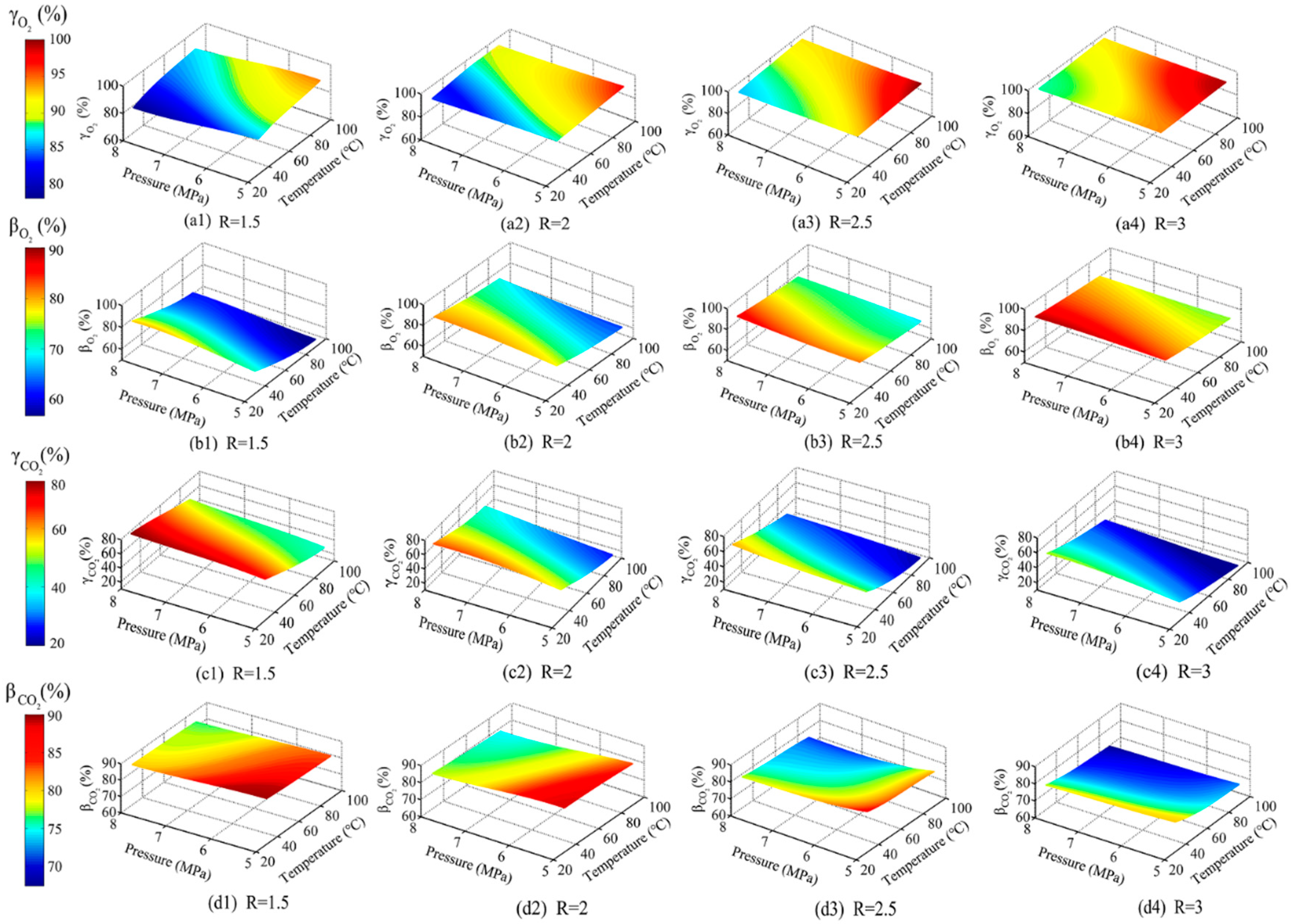
3.4. Effects of Operating Parameters
3.4.1. Stoichiometric Oxygen Excess
3.4.2. Feed Concentration
4. Aspen Model for SCWO System Simulation with Energy and Species Recovery
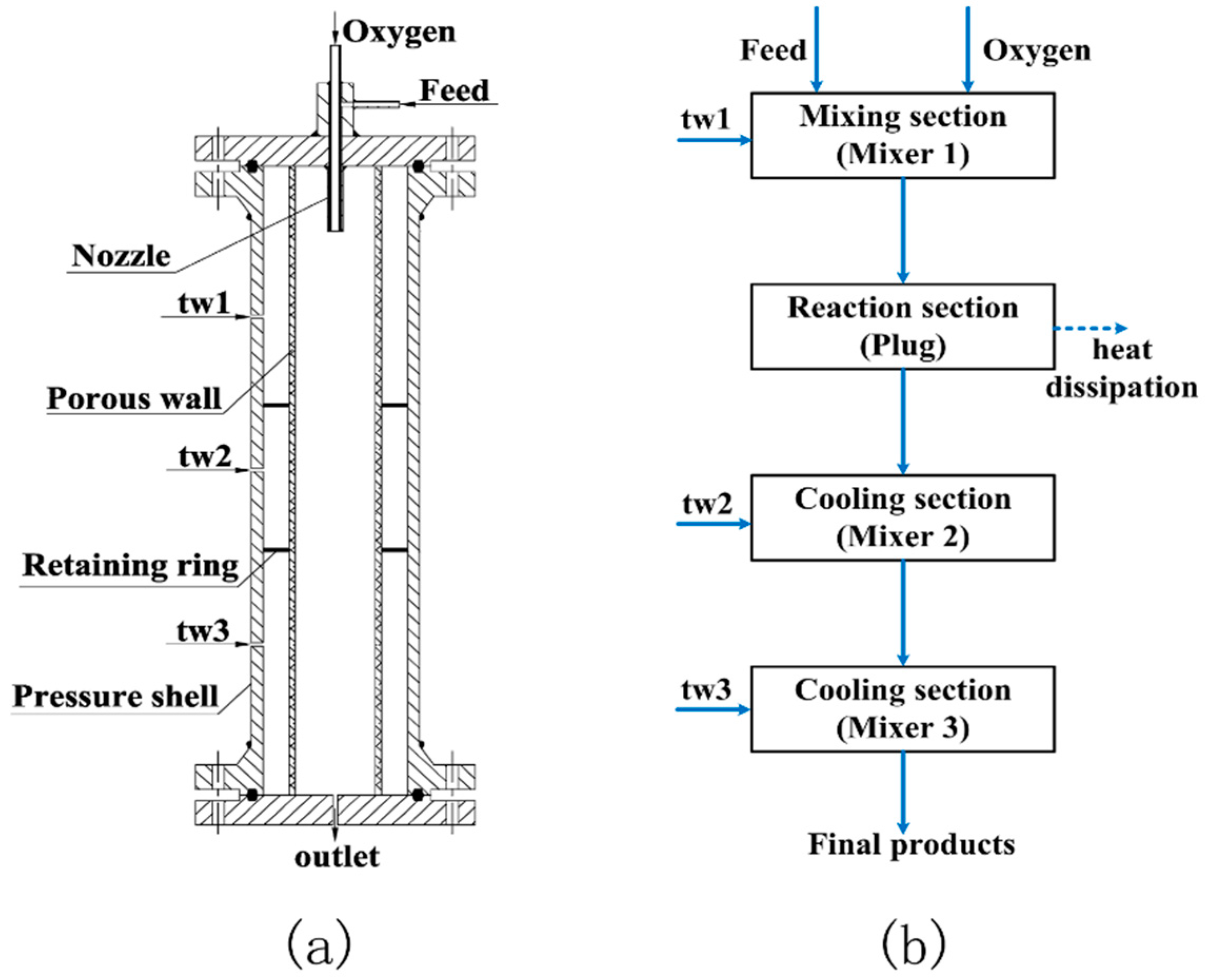
4.1. TWR
4.2. Reaction
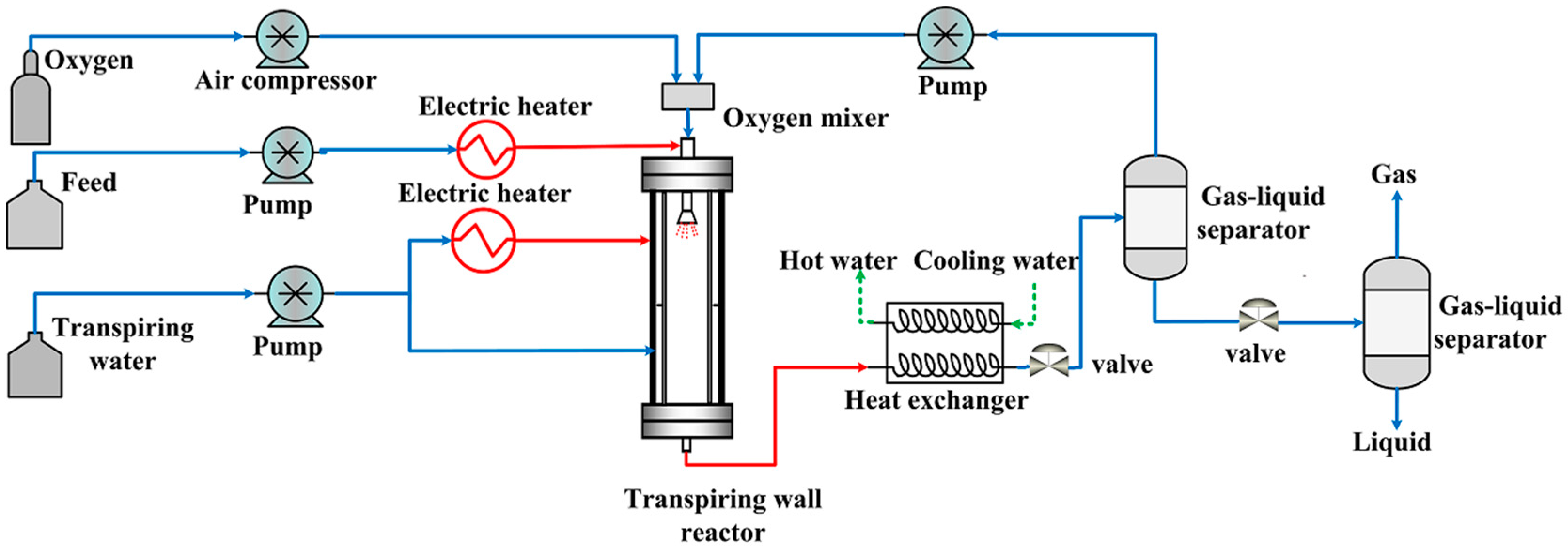
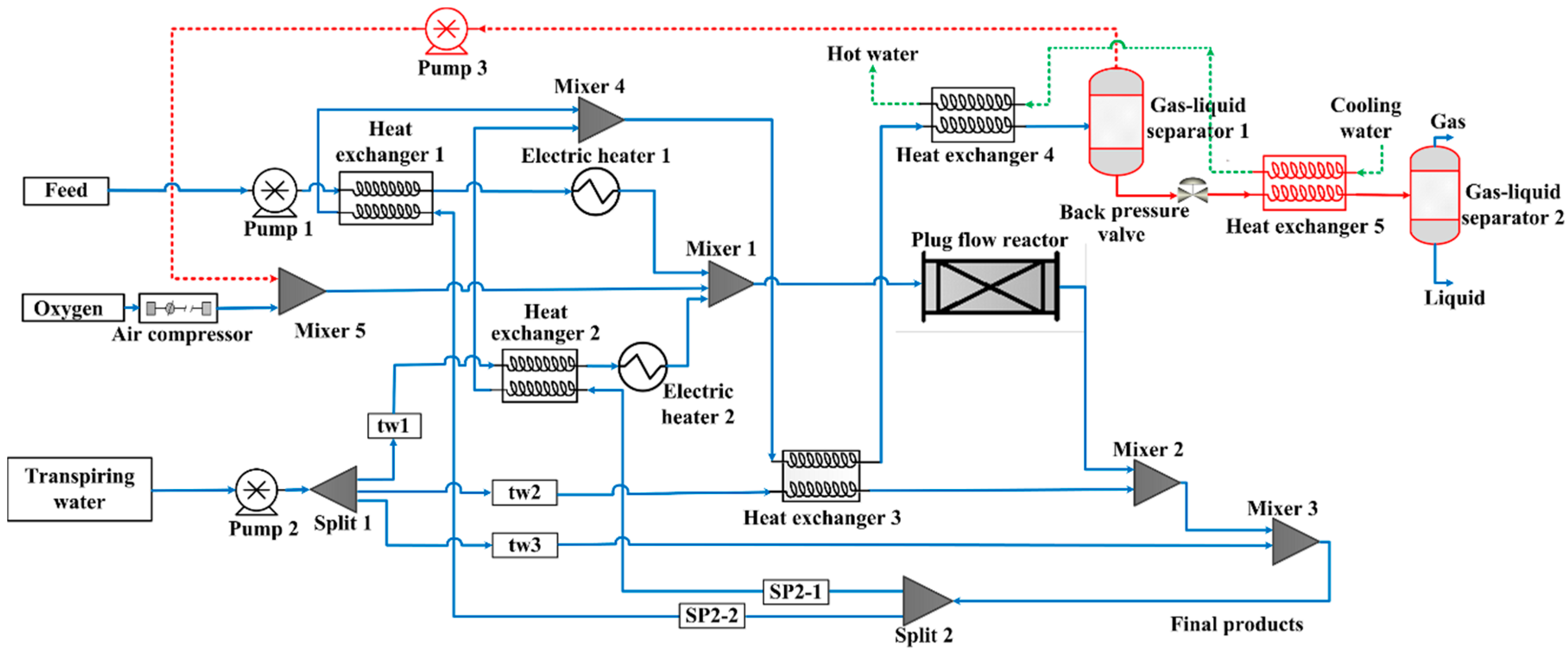
4.3. Process Flow
5. Energy and Economic Analysis
5.1. Equipment Investment Calculation
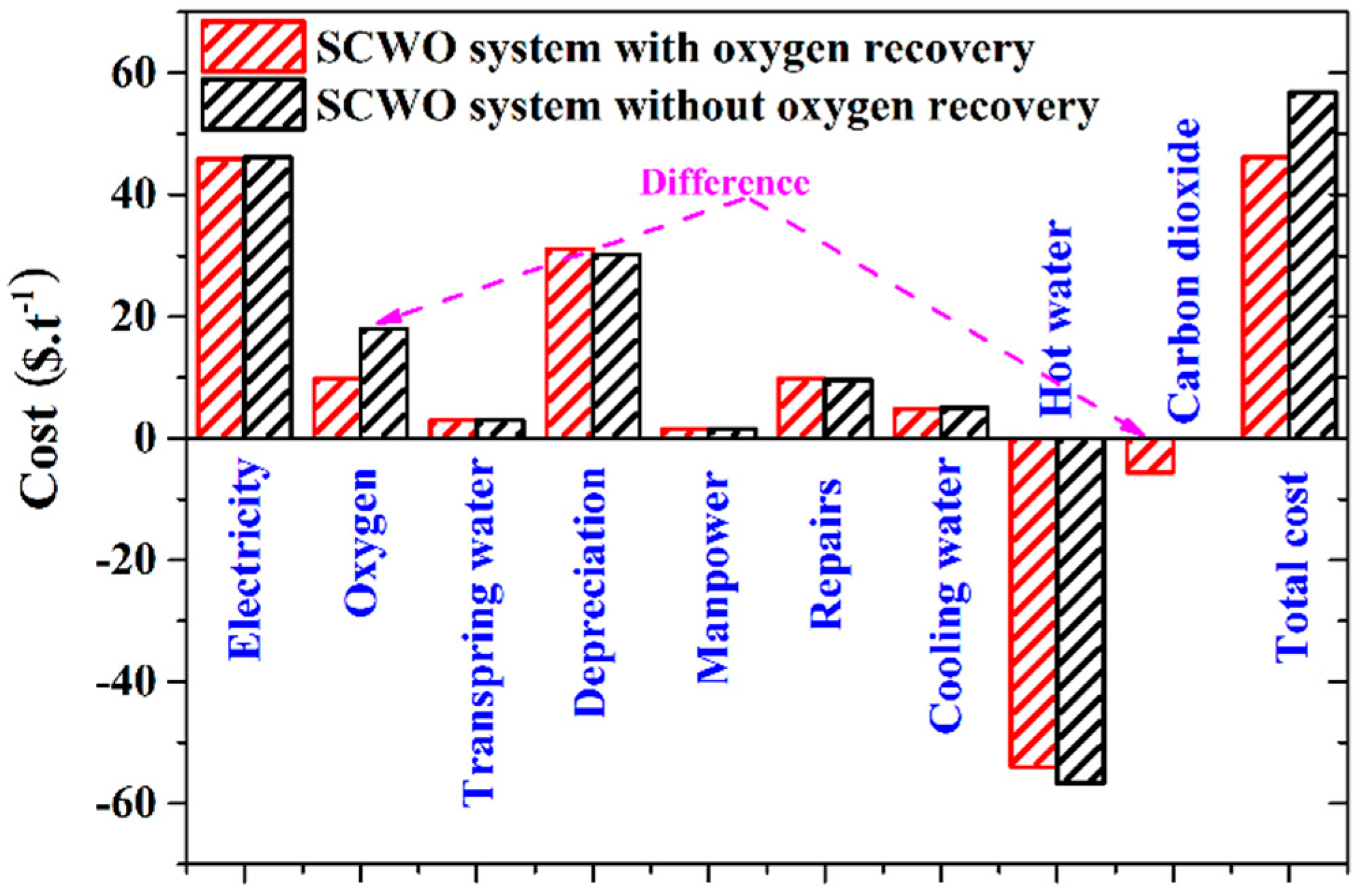
5.2. Treatment Cost Calculation and Distribution
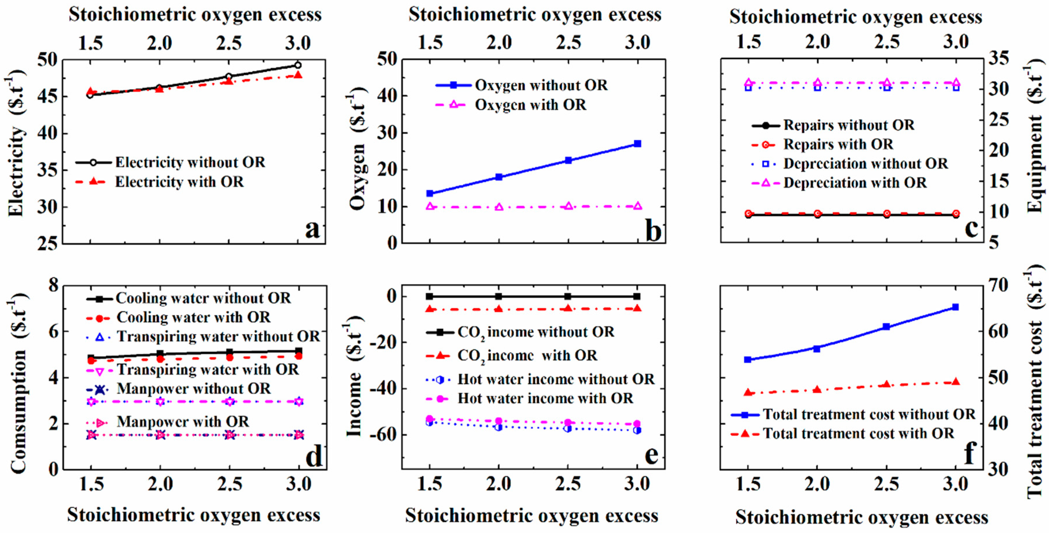
5.3. Effect of Stoichiometric Oxygen Excess
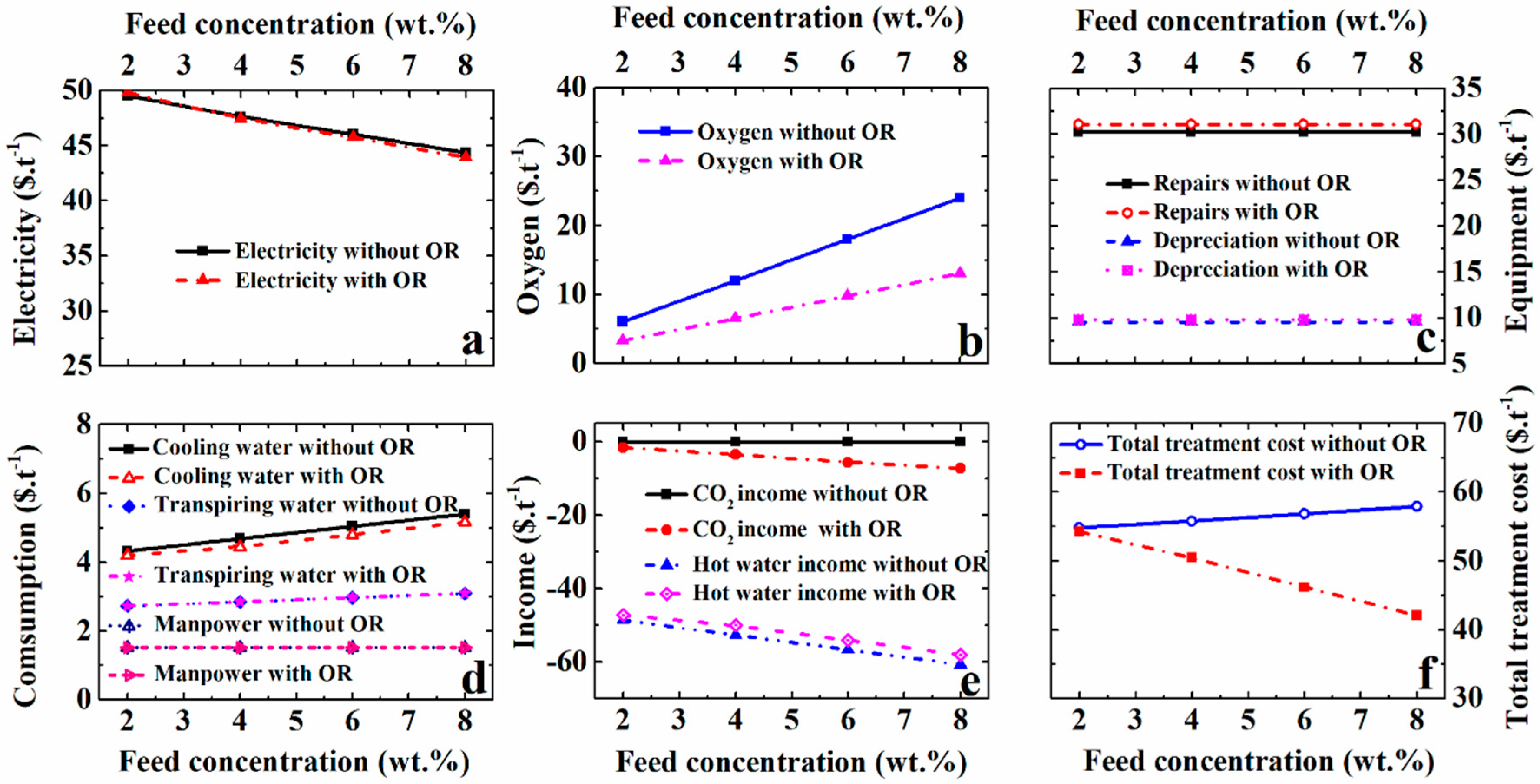
5.4. Effect of the Feed Concentration
6. Conclusions
Author Contributions
Funding
Conflicts of Interest
Nomenclature
| Abbreviations | |
| A | area |
| AC | air compressor |
| C | capital |
| COD | chemical oxygen demand |
| EH | electric heater |
| F | mass flow rate, kg·h−1 |
| FINAL | Final products |
| FP | pressure correction coefficient |
| FM | material correction coefficient |
| HE | heat exchanger |
| M | mixer |
| OR | oxygen recovery |
| P | pressure/ pump |
| R | transpiring intensity, universal gas constant |
| S | Separator |
| SCW | supercritical water |
| SCWG | supercritical water gasification |
| SCWO | supercritical water oxidation |
| r | reaction rate |
| R | stoichiometric oxygen excess |
| t | time, s |
| T | temperature, °C |
| tw1 | upper branch of transpiring water |
| tw2 | middle branch of transpiring water |
| tw3 | lower branch of transpiring water |
| TWR | transpiring wall reactor |
| TOC | total organic carbon, ppm |
| X | Design parameter |
| Greek letters | |
| β | purity |
| ρ | fluid density, kg·m−3 |
| φ | transpiring intensity |
| γ | recovery ratio |
| δ | correction coefficient |
| ω | feed concentration, wt% |
| Subscripts | |
| cw | cooling water |
| f | feed |
| g | gas |
| l | liquid |
| m | material |
| su | supplement |
| out | outlet |
| tot | total |
References
- Akiya, N.; Savage, P.E. Roles of Water for Chemical Reactions in High Temperature Water. Chem. Rev. 2002, 33, 2725–2750. [Google Scholar] [CrossRef]
- Xu, D.H.; Huang, C.B.; Wang, S.Z.; Lin, G.K.; Guo, Y. Salt deposition problems in supercritical water oxidation. Chem. Eng. J. 2015, 279, 1010–1022. [Google Scholar] [CrossRef]
- Queiroz, J.P.S.; Bermejo, M.D.; Mato, F.; Cocero, M.J. Supercritical water oxidation with hydrothermal flame as internal heat source: Efficient and clean energy production from waste. J. Supercrit. Fluid 2015, 96, 103–113. [Google Scholar] [CrossRef]
- Molino, A.; Migliori, M.; Blasi, A.; Davoli, M.; Marino, T.; Chianese, S.; Catizzone, E.; Giordano, G. Municipal waste leachate conversion via catalytic supercritical water gasification process. Fuel 2017, 206, 155–161. [Google Scholar] [CrossRef]
- Fedyaeva, O.N.; Vostrikov, A.A.; Shishkin, A.V.; Dubov, D.Y. Conjugated processes of black liquor mineral and organic components conversion in supercritical water. J. Supercrit. Fluids 2019, 143, 191–197. [Google Scholar] [CrossRef]
- Vadillo, V.; Belén García-Jarana, M.B.; Sánchez-Oneto, J.; Portela, J.R.; de la Ossa, E.J.M. Simulation of Real Wastewater Supercritical Water Oxidation at High Concentration on a Pilot Plant Scale. Ind. Eng. Chem. Res. 2011, 50, 2512–2520. [Google Scholar] [CrossRef]
- Zhang, F.M.; Chen, S.Y.; Xu, C.Y.; Chen, G.F.; Ma, C.Y. Energy consumption analysis of a transpiring-wall supercritical water oxidation pilot plant based on energy recovery. Desalin. Water Treat. 2013, 51, 7341–7352. [Google Scholar] [CrossRef]
- Fourcault, A.; García-Jarana, B.; Sánchez-Oneto, J.; Marias, F.; Portela, J.R. Supercritical water oxidation of phenol with air. Experimental results and modelling. Chem. Eng. J. 2009, 152, 227–233. [Google Scholar] [CrossRef]
- Marrone, P.A. Supercritical water oxidation-Current status of full-scale commercial activity for waste destruction. J. Supercrit. Fluid 2013, 79, 283–288. [Google Scholar] [CrossRef]
- Vadillo, V.; Sánchez-Oneto, J.; Portela, J.R.; de la Ossa, E.J.M. Problems in Supercritical Water Oxidation Process and Proposed Solutions. Ind. Eng. Chem. Res. 2013, 52, 7617–7629. [Google Scholar] [CrossRef]
- Kritzer, P. Corrosion in high-temperature and supercritical water and aqueous solutions: A review. J. Supercrit. Fluid 2004, 29, 1–29. [Google Scholar] [CrossRef]
- Hodes, M.; Marrone, P.A.; Hong, G.T.; Smith, K.A.; Tester, J.W. Salt precipitation and scale control in supercritical water oxidation–Part A: Fundamentals and research. J. Supercrit. Fluids 2004, 29, 265–288. [Google Scholar] [CrossRef]
- Zhang, F.M.; Chen, S.Y.; Xu, C.Y.; Chen, G.F.; Zhang, J.M.; Ma, C.Y. Experimental study on the effects of operating parameters on the performance of a transpiring-wall supercritical water oxidation reactor. Desalination 2012, 294, 60–66. [Google Scholar] [CrossRef]
- Bermejo, M.D.; Cocero, M.J. Supercritical water oxidation: A technical review. AIChE J. 2006, 52, 3933–3951. [Google Scholar] [CrossRef]
- Xu, D.H.; Wang, S.Z.; Huang, C.B.; Tang, X.Y.; Guo, Y. Transpiring wall reactor in supercritical water oxidation. Chem. Eng. Res. Des. 2014, 92, 2626–2639. [Google Scholar] [CrossRef]
- Kritzer, P.; Dinjus, E. An assessment of supercritical water oxidation (SCWO)-Existing problems, possible solutions and new reactor concepts. Chem. Eng. J. 2001, 83, 207–214. [Google Scholar] [CrossRef]
- Kodra, D.; Balakotaiah, V. Autothermal oxidation of dilute aqueous wastes under supercritical conditions. Ind. Eng. Chem. Res. 1994, 33, 575–580. [Google Scholar] [CrossRef]
- Lavric, E.D.; Weyten, H.; Ruyck, J.D.; Plesu, V.; Lavric, V. Delocalized organic pollutant destruction through a self-sustaining supercritical water oxidation process. Energy Convers. Manag. 2005, 46, 1345–1364. [Google Scholar] [CrossRef]
- Cocero, M.J.; Alonso, E.; Sanz, M.T.; Fdz-Polanco, F. Supercritical water oxidation process under energetically self-sufficient operation. J. Supercrit. Fluids 2002, 24, 37–46. [Google Scholar] [CrossRef]
- Bermejo, M.D.; Cocero, M.J.; Ferna´ndez-Polanco, F. A process for generating power from the oxidation of coal in supercritical water. Fuel 2004, 83, 195–204. [Google Scholar] [CrossRef]
- Marias, F.; Mancini, F.; Cansell, F.; Mercadier, J. Energy recovery in supercritical water oxidation process. Environ. Eng. Sci. 2008, 25, 123–130. [Google Scholar] [CrossRef]
- Lavric, E.D.; Weyten, H.; De Ruyck, J.; Plesu, V.; Lavric, V. Supercritical water oxidation improvements through chemical reactors energy integration. Appl. Therm. Eng. 2006, 26, 1385–1392. [Google Scholar] [CrossRef]
- Jimenez-Espadafor, F.; Portela, J.R.; Vadillo, V.; Sánchez-Oneto, J.; Becerra Villanueva, J.A.; Torres García, M.; Martínez de la Ossa, E.J. Supercritical water oxidation of oily wastes at pilot plant: Simulation for energy recovery. Ind. Eng. Chem. Res. 2011, 50, 775–784. [Google Scholar] [CrossRef]
- Zhang, F.M.; Shen, B.Y.; Su, C.J.; Xu, C.Y.; Ma, J.N.; Xiong, Y.; Ma, C.Y. Energy consumption and exergy analyses of a supercritical water oxidation system with a transpiring wall reactor. Energy Convers. Manag. 2017, 145, 82–92. [Google Scholar] [CrossRef]
- Xu, D.H.; Wang, S.Z.; Gong, Y.M.; Guo, Y.; Tang, X.Y.; Ma, H.H. A demonstration plant for treating sewage sludge by supercritical water oxidation and its economic analysis. Mod. Chem. Ind. 2009, 29, 55–59. [Google Scholar]
- Zhang, J.; Wang, S.Z.; Lu, J.L.; Chen, S.L.; Li, Y.H.; Ren, M.M. A system for treating high concentration textile wastewater and sludge by supercritical water oxidation and its economic analysis. Mod. Chem. Ind. 2016, 36, 154–158. [Google Scholar]
- Shen, X.F.; Ma, C.Y.; Wang, Z.Q.; Chen, G.F.; Chen, S.Y.; Zhang, J.M.; Yi, B.K. Economic analysis of organic waste liquid treatment through supercritical water oxidation system. Environ. Eng. 2010, 28, 47–51. [Google Scholar]
- Abeln, J.; Kluth, M.; Pagel, M. Results and rough costestimation for SCWO of painting effluents using a transpiring wall and a pipe reactor. J. Adv. Oxid. Technol. 2007, 10, 169–176. [Google Scholar]
- Baranenko, V.I.; Fal’kovskii, L.N.; Kirov, V.S.; Kurnyk, L.N.; Musienko, A.N.; Piontkovskii, A.I. Solubility of oxygen and carbon dioxide in water. At. Energy 1990, 68, 342–346. [Google Scholar] [CrossRef]
- Ma, C.Y.; Zhang, F.M.; Chen, S.Y.; Chen, G.F.; Zhang, J.M. A Method of Improving Oxygen Utilization Rate in Supercritical Water Oxidation System. Chinese Patent ZL 201010174846.9, 18 May 2010. [Google Scholar]
- Holderbaum, T.; Gmehling, J. PSRK: A group contribution equation of state based on UNIFAC. Fluid Phase Equilib. 1991, 70, 251–265. [Google Scholar] [CrossRef]
- Zhang, F.M.; Xu, C.Y.; Zhang, Y.; Chen, S.Y.; Chen, G.; Ma, C.Y. Experimental study on the operating characteristics of an inner preheating transpiring wall reactor for supercritical water oxidation: Temperature profiles and product properties. Energy 2014, 66, 577–587. [Google Scholar] [CrossRef]
- Li, L.; Chen, P.; Gloyna, E.F. Generalized kinetic model for wet oxidation of organic compounds. AIChE J. 1991, 37, 1687–1697. [Google Scholar] [CrossRef]
- Vogel, F.; Blanchard, J.L.D.; Marrone, P.A.; Rice, S.F.; Webley, P.A.; Peters, W.A.; Smith, K.A.; Tester, J.W. Critical review of kinetic data for the oxidation of methanol in supercritical water. J. Supercrit. Fluid 2005, 34, 249–286. [Google Scholar] [CrossRef]
- Dagaut, P.; Cathonnet, M.; Boettner, J. Chemical Kinetic Modeling of the Supercritical-Water Oxidation of Methanol. J. Supercrit. Fluids 1996, 98, 33–42. [Google Scholar] [CrossRef]
- Tester, J.W.; Webley, P.A.; Holgate, H.R. Revised global kinetic measurements of methanol oxidation in supercritical water. Ind. Eng. Chem. Res. 1993, 32, 236–239. [Google Scholar] [CrossRef]
- Turton, R.; Bailie, R.C.; Whiting, W.B.; Bhattacharyya, D. Analysis, Synthesis and Design of Chemical Processes; Prentice Hall: Upper Saddle River, NJ, USA, 2012. [Google Scholar]
- Shen, X.F. Design and Technical Economic Analysis on Heat Supply System by Supercritical Water Oxidation Energy Conversion. Master’s Thesis, Shandong University, Jinan, China, 2009. [Google Scholar]
- Wildi-Tremblay, P.; Gosselin, L. Minimizing shell-and-tube heat exchanger cost with genetic algorithms and considering maintenance. Int. J. Energy Res. 2007, 31, 867–888. [Google Scholar] [CrossRef]
- Zhang, F.M.; Zhang, Y.; Xu, C.Y.; Chen, S.Y.; Chen, G.F.; Ma, C.Y. Experimental study on the ignition and extinction characteristics of the hydrothermal flame. Chem. Eng. Technol. 2015, 38, 2054–2066. [Google Scholar] [CrossRef]


| Aspen Plus Property Model | Model Name |
|---|---|
| BWR-LS | Benedict-Webb-Rubin-Lee-Starling |
| PR-BM | Peng-Robinson-Boston-Mathias |
| SR-POLAR | Schwarzentruber-Renon-POLAR |
| SRK | Soave-Redlich-Kwong |
| PSRK | Predictive Redlich-Kwong-Soave |
| RKS-BM | Redlich-Kwong-Soave-Boston-Mathias |
| LK-Plock | Lee-Kesler-Plock |
| RK-SWS | Redlich-Kwong-Soave-Wong-Sandler |
| PR-MHV2 | Peng-Robinson-MHV2 |
| PR-WS | Peng-Robinson-Wong-Sandler |
| RKS-MHV2 | Redlich-Kwong-Soave-MHV2 |
| R α | ω β (wt%) | FO2 (kg·h−1) | FCO2γ (kg·h−1) | FH2Oδ (kg·h−1) | P’ /MPa | T’ (°C) | F’O2,g (kg·h−1) | F’CO2,g (kg·h−1) | F’H2O,g (kg·h−1) | γO2 (%) | βO2 (%) | P’’ /MPa | T’’ (°C) | F’CO2,l (kg·h−1) | F’O2,l (kg·h−1) | F’’O2,g (kg·h−1) | F’’CO2,g (kg·h−1) | γCO2 (%) | βCO2 (%) | |
|---|---|---|---|---|---|---|---|---|---|---|---|---|---|---|---|---|---|---|---|---|
| A1 | 1.5 | 6 | 0.450 | 0.825 | 37.820 | 6–7 | 30–40 | 0.353–0.385 | 0.122–0.21 | <0.018 | 78.6–85.7 | 70.6–78.6 | 0.1 | 20 | 0.616–0.704 | 0.064–0.096 | 0.064–0.096 | 0.572–0.616 | 68.42–73.68 | 82.4–87.5 |
| A2 ε | 2.0 | 6 | 0.900 | 0.825 | 39.293 | 6–7 | 30–40 | 0.803–0.835 | 0.254–0.340 | <0.018 | 89.3–92.86 | 76.5–80.6 | 0.1 | 20 | 0.484–0.572 | 0.064–0.096 | 0.064–0.096 | 0.44–0.528 | 52.63–63.16 | 80–84.62 |
| A3 | 2.5 | 6 | 1.350 | 0.825 | 40.766 | 6–7 | 30–40 | 1.252–1.283 | 0.342–0.430 | <0.018 | 92.86–95.24 | 80–83.1 | 0.1 | 20 | 0.396–0.484 | 0.064–0.096 | 0.064–0.096 | 0.35–0.442 | 42.10–53.63 | 76–81.1 |
| A4 | 3.0 | 6 | 1.800 | 0.825 | 42.239 | 6–7 | 30–40 | 1.699–1.730 | 0.386–0.474 | <0.018 | 94.6–96.43 | 83.1–85.5 | 0.1 | 20 | 0.352–0.44 | 0.064–0.096 | 0.064–0.096 | 0.308–0.396 | 36.84–47.36 | 73–80 |
| B1 | 2.0 | 2 | 0.300 | 0.275 | 34.916 | 5 | 60–70 | 0.234–0.266 | 0.054–0.098 | <0.018 | 78–89 | 82–86 | 0.1 | 20 | 0.176–0.22 | 0.032–0.064 | 0.032 | 0.132–0.176 | 50.00–66.67 | 75–80 |
| B2 | 2.0 | 4 | 0.600 | 0.550 | 37.105 | 6 | 30–40 | 0.540 | 0.112–0.156 | <0.018 | 89.5 | 81–84 | 0.1 | 20 | 0.396–0.44 | 0.064 | 0.064 | 0.352–0.396 | 64.58–69.23 | 80–82 |
| B3 | 2.0 | 6 | 0.900 | 0.825 | 39.293 | 6–7 | 30–40 | 0.800–0.832 | 0.254–0.340 | <0.018 | 89.3–92.86 | 76.5–80.6 | 0.1 | 20 | 0.484–0.572 | 0.064–0.096 | 0.064–0.096 | 0.44–0.528 | 52.63–63.16 | 80–84.62 |
| B4 | 2.0 | 8 | 1.200 | 1.100 | 41.482 | 6–8 | 30–40 | 1.107–1.142 | 0.396–0.528 | <0.018 | 92.1–94.7 | 75–80 | 0.1 | 20 | 0.572–0.704 | 0.064–0.096 | 0.064–0.096 | 0.528–0.66 | 48.00–60.00 | 81.25–86.7 |
| B5 | 2.0 | 10 | 1.500 | 1.375 | 43.670 | 6–8 | 30–40 | 1.408–1.420 | 0.582–0.758 | <0.018 | 93.62–95.7 | 73–77.2 | 0.1 | 20 | 0.616–0.792 | 0.064–0.096 | 0.064–0.096 | 0.572–0.748 | 41.93–54.84 | 82.4–88.2 |
| NO | R | ω (wt%) | Ff (kg·h−1) | Ftw1a (kg·h−1) | Ftw2 (kg·h−1) | Ftw3 (kg·h−1) | Fcwb (kg·h−1) | FFinal (kg·h−1) | Fsp2-1c (kg·h−1) | Fsp2-2 (kg·h−1) | FO2,tot (kg·h−1) | FO2,re (kg·h−1) | FO2,su (kg·h−1) | FCO2,re (kg·h−1) | TEH1d (°C) | TEH2 (°C) | TEH3 (°C) | Tf (°C) | Ttw1 (°C) | Ttw2 (°C) | TM1 (°C) | Tout (°C) | Tsp2-1 (°C) | Tsp2-2 (°C) | TM4 (°C) | COout (%) | TOCout /ppm | γO2 (%) | γCO2 (%) | βO2 (%) | βCO2 (%) | |
|---|---|---|---|---|---|---|---|---|---|---|---|---|---|---|---|---|---|---|---|---|---|---|---|---|---|---|---|---|---|---|---|---|
| With oxygen recovery | A1 | 1.5 | 6 | 1000 | 1857 | 620 | 1236 | 19,700 | 4927 | 2956 | 1970 | 135 | 35.8 | 99.2 | 79.2 | 301 | 301 | 181 | 380 | 350 | 160 | 360 | 333 | 191 | 223 | 204 | 0 | 0 | 79.56 | 73.7 | 73.89 | 86.78 |
| A2e | 2 | 6 | 1000 | 1931 | 644 | 1287 | 20,000 | 5121 | 3072 | 2048 | 180 | 82.1 | 97.9 | 79.2 | 300 | 300 | 179 | 380 | 350 | 159 | 357 | 331 | 188 | 220 | 201 | 0 | 0 | 91.22 | 58.4 | 77.89 | 82.13 | |
| A3 | 2.5 | 6 | 1000 | 2005 | 668 | 1336 | 20,250 | 5308 | 3185 | 2123 | 225 | 124.8 | 100.2 | 74.8 | 299 | 299 | 179 | 381 | 350 | 158 | 355 | 330 | 189 | 221 | 202 | 0 | 0 | 92.44 | 47.4 | 81.56 | 78.89 | |
| A4 | 3 | 6 | 1000 | 2078 | 693 | 1385 | 20,500 | 5500 | 3300 | 2200 | 270 | 169.95 | 100.05 | 74.8 | 298 | 298 | 178 | 382 | 350 | 161 | 352 | 328 | 190 | 221 | 203 | 0 | 0 | 94.42 | 42.1 | 84.39 | 74.56 | |
| B1 | 2 | 2 | 1000 | 1735 | 578 | 1156 | 17,500 | 4551 | 2731 | 1820 | 60 | 20.61 | 39.39 | 22.1 | 296 | 296 | 155 | 390 | 350 | 150 | 368 | 316 | 161 | 183 | 170 | 0 | 0 | 79.2 | 68.91 | 85.89 | 80.21 | |
| B2 | 2 | 4 | 1000 | 1832 | 611 | 1222 | 18,500 | 4833 | 2900 | 1933 | 120 | 53.64 | 66.36 | 48.4 | 298 | 298 | 165 | 385 | 350 | 155 | 363 | 324 | 175 | 204 | 187 | 0 | 0 | 89.4 | 62.14 | 82.36 | 81.34 | |
| B3 | 2 | 6 | 1000 | 1931 | 644 | 1287 | 20,000 | 5121 | 3073 | 2048 | 180 | 82.1 | 97.9 | 79.2 | 300 | 300 | 179 | 380 | 350 | 159 | 357 | 331 | 188 | 220 | 201 | 0 | 0 | 91.22 | 58.4 | 77.89 | 82.13 | |
| B4 | 2 | 8 | 1000 | 2029 | 676 | 1353 | 21,500 | 5399 | 3239 | 2160 | 240 | 113.64 | 126.36 | 101.2 | 303 | 302 | 194 | 376 | 350 | 167 | 352 | 335 | 198 | 236 | 214 | 0 | 0 | 94.7 | 52.1 | 76.20 | 84.36 | |
| Without oxygen recovery | C1 | 1.5 | 6 | 1000 | 1857 | 620 | 1236 | 20,200 | 4848 | 2908 | 1939 | 135 | - | - | - | 301 | 301 | 182 | 380 | 350 | 161 | 361 | 334 | 192 | 224 | 205 | 0 | 0 | - | - | - | - |
| C2 | 2 | 6 | 1000 | 1931 | 644 | 1287 | 21,000 | 5042 | 3025 | 2016 | 180 | - | - | - | 300 | 300 | 181 | 380 | 350 | 160 | 360 | 333 | 190 | 223 | 204 | 0 | 0 | - | - | - | - | |
| C3 | 2.5 | 6 | 1000 | 2005 | 668 | 1336 | 21,200 | 5234 | 3140 | 2093 | 225 | - | - | - | 299 | 299 | 180 | 381 | 350 | 159 | 356 | 330 | 189 | 221 | 202 | 0 | 0 | - | - | - | - | |
| C4 | 3 | 6 | 1000 | 2078 | 693 | 1385 | 21,500 | 5426 | 3255 | 2170 | 270 | - | - | - | 298 | 298 | 180 | 382 | 350 | 161 | 354 | 330 | 190 | 222 | 203 | 0 | 0 | - | - | - | - | |
| D1 | 2 | 2 | 1000 | 1735 | 578 | 1156 | 18,000 | 4529 | 2717 | 1812 | 60 | - | - | - | 297 | 296 | 156 | 390 | 350 | 150 | 368 | 316 | 161 | 183 | 170 | 0 | 0 | - | - | - | - | |
| D2 | 2 | 4 | 1000 | 1832 | 611 | 1222 | 19,500 | 4785 | 2871 | 1914 | 120 | - | - | - | 299 | 298 | 167 | 385 | 350 | 155 | 364 | 325 | 175 | 204 | 187 | 0 | 0 | - | - | - | - | |
| D3 | 2 | 6 | 1000 | 1931 | 644 | 1287 | 21,000 | 5042 | 3025 | 2017 | 180 | - | - | - | 300 | 300 | 181 | 380 | 350 | 160 | 360 | 333 | 190 | 223 | 204 | 0 | 0 | - | - | - | - | |
| D4 | 2 | 8 | 1000 | 2029 | 676 | 1353 | 22,500 | 5298 | 3179 | 2119 | 240 | - | - | - | 302 | 302 | 195 | 376 | 350 | 168 | 354 | 337 | 199 | 237 | 215 | 0 | 0 | - | - | - | - |
| Equipment | K1 | K2 | K3 | C1 | C2 | C3 | B1 | B2 | FP | FM |
|---|---|---|---|---|---|---|---|---|---|---|
| Reactor | 4.7116 | 0.4479 | 0.0004 | - | - | - | - | - | - | 4 |
| Pump | 3.8696 | 0.3161 | 0.1220 | −0.3935 | 0.3957 | −0.0023 | 1.89 | 1.35 | 2.2 | - |
| Electric heater | 1.1979 | 1.4782 | −0.0958 | −0.01635 | 0.05687 | −0.00876 | - | - | - | 1.4 |
| Compressor | 2.2897 | 1.3604 | −0.1027 | 0 | 0 | 0 | - | - | 2.2 | - |
| Gas-liquid separator | 3.4974 | 0.4485 | 0.1074 | - | - | - | 1.49 | 1.52 | - | 1.25 |
| Equipment | Temperature (°C) | Pressure (MPa) | Material | δM | δP | δT |
|---|---|---|---|---|---|---|
| Heat exchanger 1 | 500 | 30 | Stainless steel 316L | 2.9 | 1.9 | 2.1 |
| Heat exchanger 2 | 500 | 30 | Stainless steel 316L | 2.9 | 1.9 | 2.1 |
| Heat exchanger 3 | 500 | 30 | Stainless steel 316L | 2.9 | 1.9 | 2.1 |
| Heat exchanger 4 | 300 | 30 | Stainless steel 316L | 2.9 | 1.9 | 1.6 |
| NO | Equipment | Parameter | SCWO System with Oxygen Recovery | SCWO without Oxygen Recovery | ||||||
|---|---|---|---|---|---|---|---|---|---|---|
| Theoretical Value | Safety Factor a | Design Value | Cost ($) | Theoretical Value | Safety Factor a | Design Value | Cost ($) | |||
| 1 | Heat exchanger 1 | Area/m2 | 5.77 | 1.2 | 7 | 72,412 | 5.76 | 1.2 | 7 | 72,412 |
| 2 | Heat exchanger 2 | Area/m2 | 12.26 | 1.2 | 15 | 121,586 | 12.24 | 1.2 | 15 | 121,586 |
| 3 | Heat exchanger 3 | Area/m2 | 1.146 | 1.2 | 1.5 | 25,403 | 1.14 | 1.2 | 1.5 | 25,403 |
| 4 | Heat exchanger 4 | Area/m2 | 19.73 | 1.2 | 24 | 127,522 | 22.5 | 1.2 | 27 | 143,166 |
| 5 | Heat exchanger 5 | Area/m2 | 3.78 | 1.2 | 4.5 | 25,533 | -- | -- | -- | -- |
| 6 | Waste water pump | Power/kW | 11.28 | 1.2 | 14 | 155,452 | 11.28 | 1.2 | 14 | 155,452 |
| 7 | Compressor b | Power/kW | 36.88 | 1.6 | 60 | 132,840 | 36.88 | 1.6 | 60 | 132,840 |
| 8 | Transpiring water pump | Power/kW | 41.32 | 1.2 | 50 | 145,800 | 41.32 | 1.2 | 50 | 145,800 |
| 9 | Oxygen circulation pump | Power/kW | 4.59 | 2.1 | 9.5 | 21,034 | -- | -- | -- | -- |
| 10 | Transpiring wall reactor | Volume/m3 | 0.695 | 3 | 2.1 | 531,798 | 0.695 | 3 | 2.1 | 531,798 |
| 11 | High-pressure separator | Volume/m3 | 0.189 | 3 | 0.6 | 7142 | -- | -- | -- | -- |
| 12 | Low-pressure separator | Volume/m3 | 0.186 | 1.5 | 0.3 | 3570 | 0.189 | 1.5 | 0.3 | 3570 |
| 13 | Electric heater 1 | Power/kW | 306.81 | 1.2 | 370 | 31,365 | 306.81 | 1.2 | 370 | 31,365 |
| 14 | Electric heater 2 | Power/kW | 190.56 | 1.2 | 228 | 19,380 | 190.56 | 1.2 | 228 | 19,380 |
| 15 | Total equipment cost/1996 | $ | 1,420,837 | 1,382,772 | ||||||
| 16 | Total equipment cost/2016 | $ | 2,253,997 | 2,193,612 | ||||||
| 17 | Installation cost c | $ | 338,099 | 329,042 | ||||||
| 18 | Total investment cost/2016 | $ | 2,592,096 | 2,522,654 | ||||||
| R | ω(wt%) | P1(kW) | PAC(kW) | P2(kW) | P3(kW) | PEH1(kW) | PEH2(kW) | Total(kW) | ||
|---|---|---|---|---|---|---|---|---|---|---|
| With oxygen recovery | A1 | 1.5 | 6 | 11.28 | 25.6 | 41.31 | 2.23 | 306.81 | 190.56 | 577.79 |
| A2 | 2 | 6 | 11.28 | 24.53 | 42.95 | 4.59 | 306.81 | 190.56 | 580.08 | |
| A3 | 2.5 | 6 | 11.28 | 26.12 | 44.59 | 6.67 | 312.89 | 193.38 | 594.93 | |
| A4 | 3 | 6 | 11.28 | 26.05 | 46.22 | 8.99 | 316.87 | 196.47 | 605.88 | |
| B1 | 2 | 2 | 11.18 | 11.89 | 38.05 | 1.56 | 361.4 | 206.32 | 630.4 | |
| B2 | 2 | 4 | 11.23 | 16.71 | 39.70 | 2.82 | 331.45 | 198.15 | 600.06 | |
| B3 | 2 | 6 | 11.28 | 24.53 | 42.95 | 4.59 | 306.81 | 190.56 | 580.08 | |
| B4 | 2 | 8 | 11.34 | 30.66 | 43.97 | 6.45 | 281.64 | 182.82 | 556.88 | |
| Without Oxygen recovery | C1 | 1.5 | 6 | 11.28 | 27.66 | 41.31 | - | 302.11 | 190.01 | 572.37 |
| C2 | 2 | 6 | 11.28 | 36.88 | 42.95 | - | 304.24 | 189.26 | 583.97 | |
| C3 | 2.5 | 6 | 11.28 | 46.10 | 44.59 | - | 310.19 | 191.98 | 604.14 | |
| C4 | 3 | 6 | 11.28 | 55.32 | 46.22 | - | 315.77 | 195.17 | 623.76 | |
| D1 | 2 | 2 | 11.18 | 12.29 | 38.05 | - | 360.40 | 204.82 | 626.74 | |
| D2 | 2 | 4 | 11.23 | 24.59 | 39.70 | - | 329.34 | 197.61 | 602.47 | |
| D3 | 2 | 6 | 11.28 | 36.88 | 42.95 | - | 304.24 | 189.26 | 583.97 | |
| D4 | 2 | 8 | 11.34 | 49.18 | 43.97 | - | 277.14 | 180.82 | 562.45 |
© 2018 by the authors. Licensee MDPI, Basel, Switzerland. This article is an open access article distributed under the terms and conditions of the Creative Commons Attribution (CC BY) license (http://creativecommons.org/licenses/by/4.0/).
Share and Cite
Zhang, F.; Chen, J.; Su, C.; Ma, C. Energy Consumption and Economic Analyses of a Supercritical Water Oxidation System with Oxygen Recovery. Processes 2018, 6, 224. https://doi.org/10.3390/pr6110224
Zhang F, Chen J, Su C, Ma C. Energy Consumption and Economic Analyses of a Supercritical Water Oxidation System with Oxygen Recovery. Processes. 2018; 6(11):224. https://doi.org/10.3390/pr6110224
Chicago/Turabian StyleZhang, Fengming, Jiulin Chen, Chuangjian Su, and Chunyuan Ma. 2018. "Energy Consumption and Economic Analyses of a Supercritical Water Oxidation System with Oxygen Recovery" Processes 6, no. 11: 224. https://doi.org/10.3390/pr6110224
APA StyleZhang, F., Chen, J., Su, C., & Ma, C. (2018). Energy Consumption and Economic Analyses of a Supercritical Water Oxidation System with Oxygen Recovery. Processes, 6(11), 224. https://doi.org/10.3390/pr6110224