Waste Fuel Combustion: Dynamic Modeling and Control


Abstract
1. Introduction
1.1. Modelling and Control
1.1.1. Modeling
- Level I: The 1D approach, the boiler is considered to be either a plug flow or stirred tank and mass and energy balances are used to describe the phenomena occurring.
- Level II: The boiler region is split into core and annulus regions, quasi-2D model, to incorporate the changes in solid and gas temperatures and concentrations to achieve a higher resolution.
- Level III: The combustion process is based on the Navier–Stokes equation, a 3D model, and chemical kinetics and physical processes are incorporated in detail.
1.1.2. Control
1.2. Aim and Contribution
- Can a dynamic modeling library for the the combustion of waste fuel, based on first principle modeling techniques, be used to improve RDF fired CFB plant operations?
- To what degree does implementing feedforward MPC on a waste-fired CFB compare to that of MPC without feedforward and traditional PI-control schemes?
2. Circulating Fluidized Bed Boilers
Refuse Derived Fuels
- Create a more uniform size distribution in the final RDF product,
- Sort out the recyclable fraction, i.e., metal, glass, and plastics,
- Sort out the non-combustible fraction, i.e., ceramics and rocks.
3. Model Description and Methodology
3.1. Process Parameters
3.2. Description of Model and Methodology
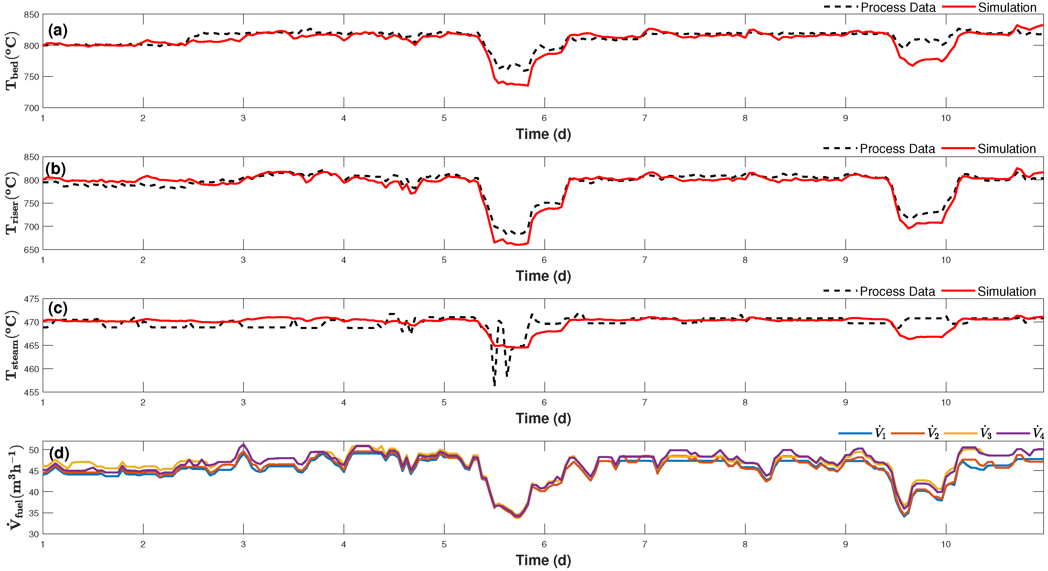
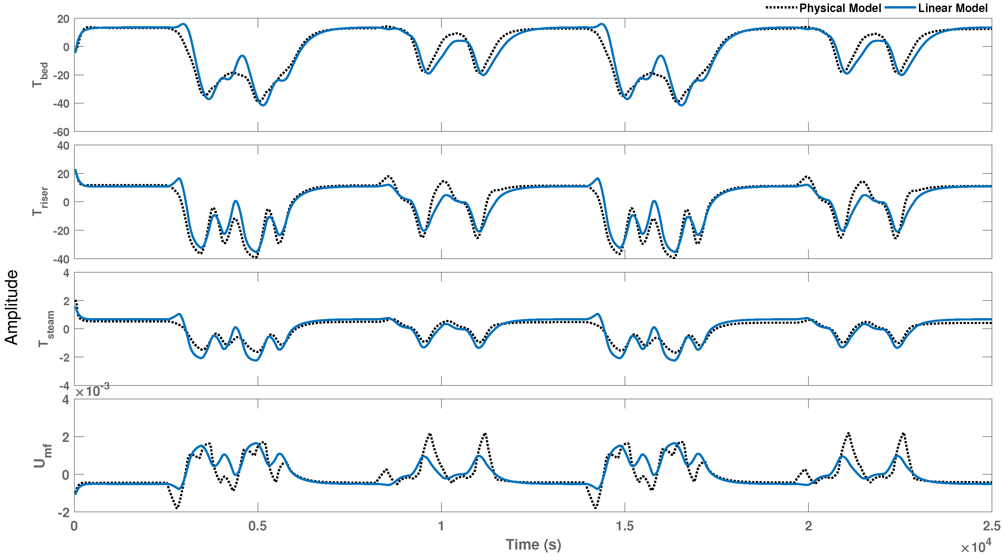
4. Validation
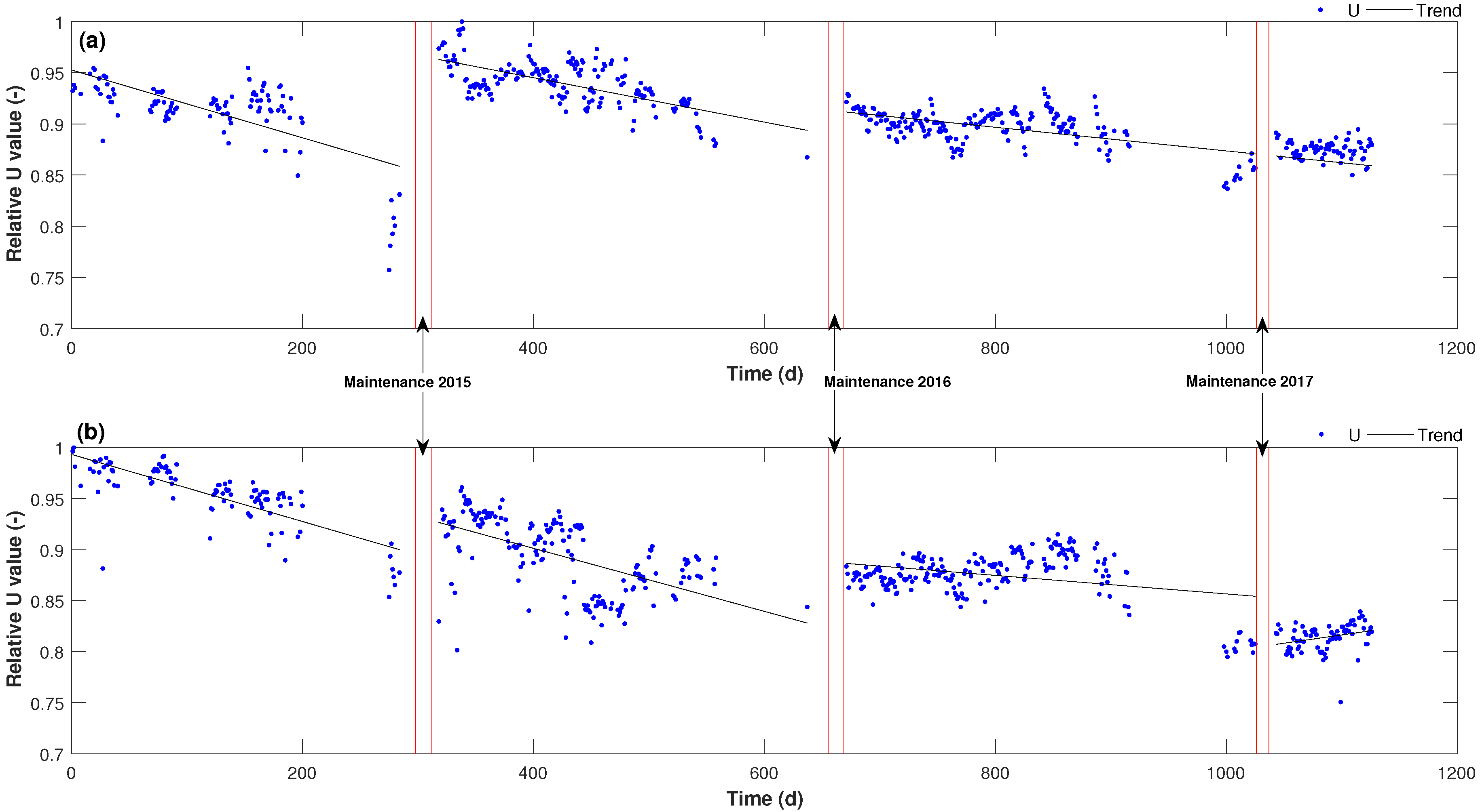
Offline Process Monitoring
5. Results and Discussion
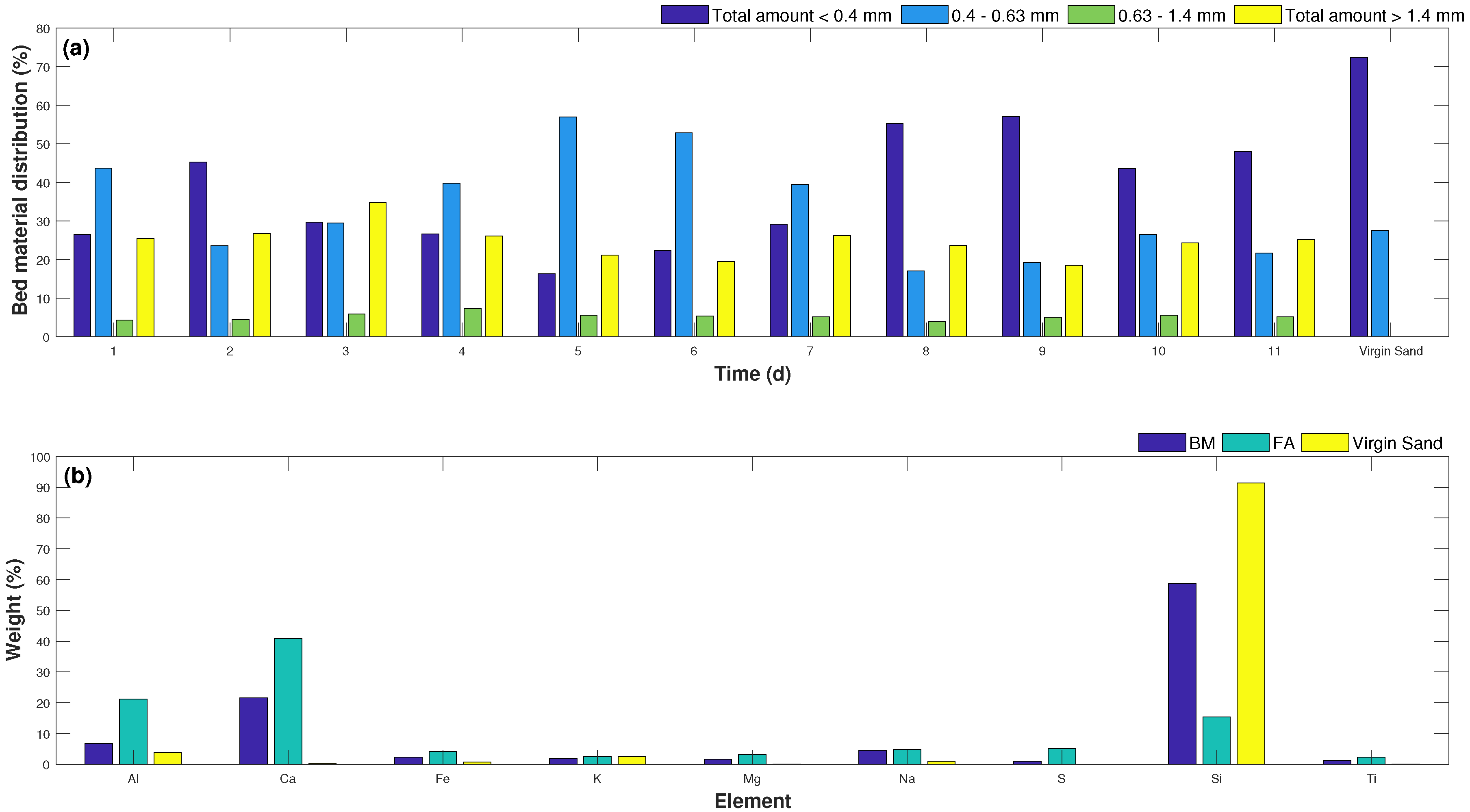
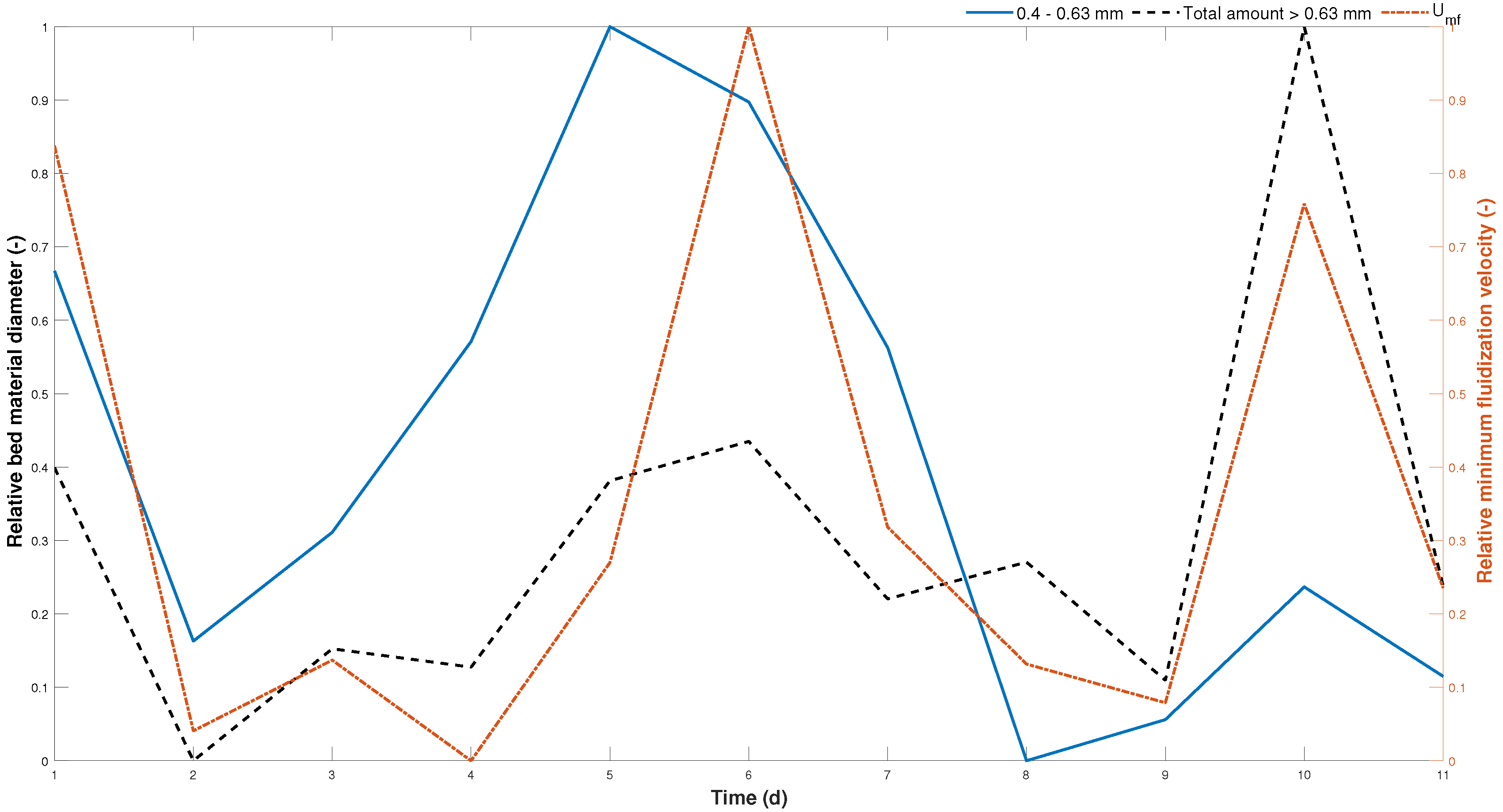
5.1. Agglomeration
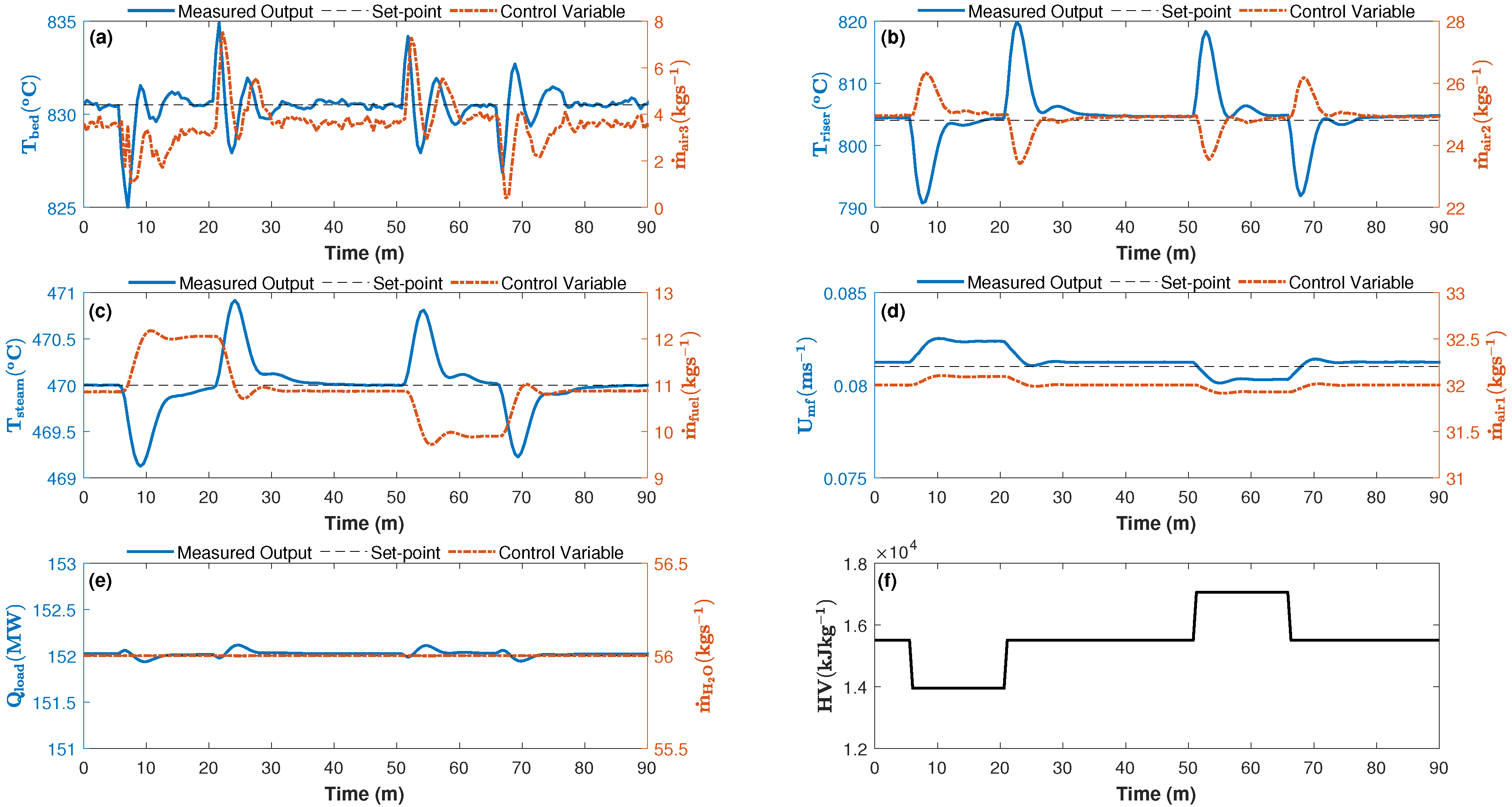
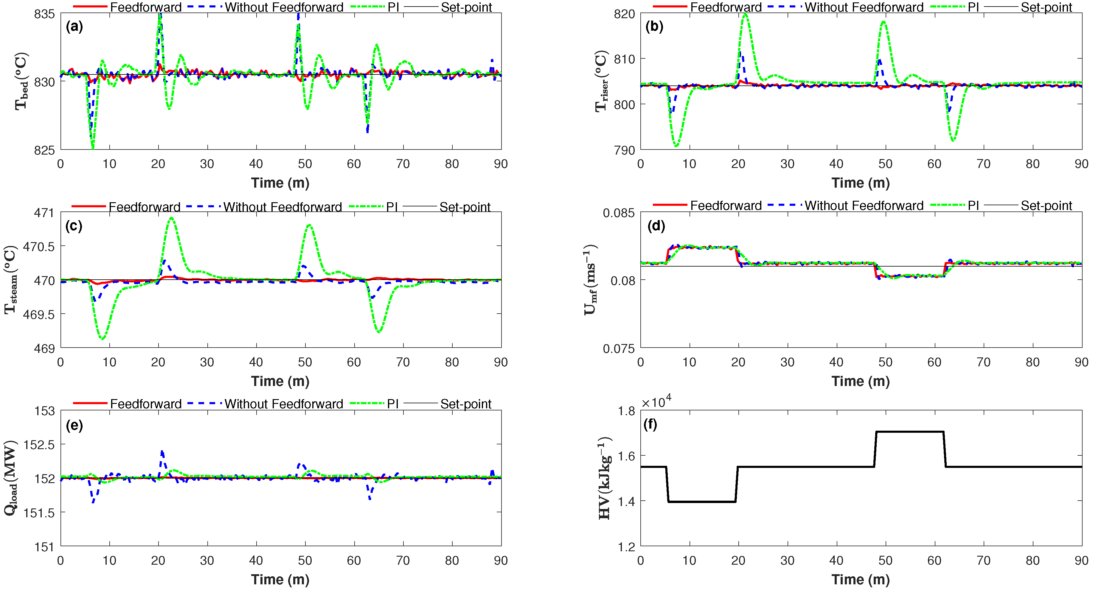
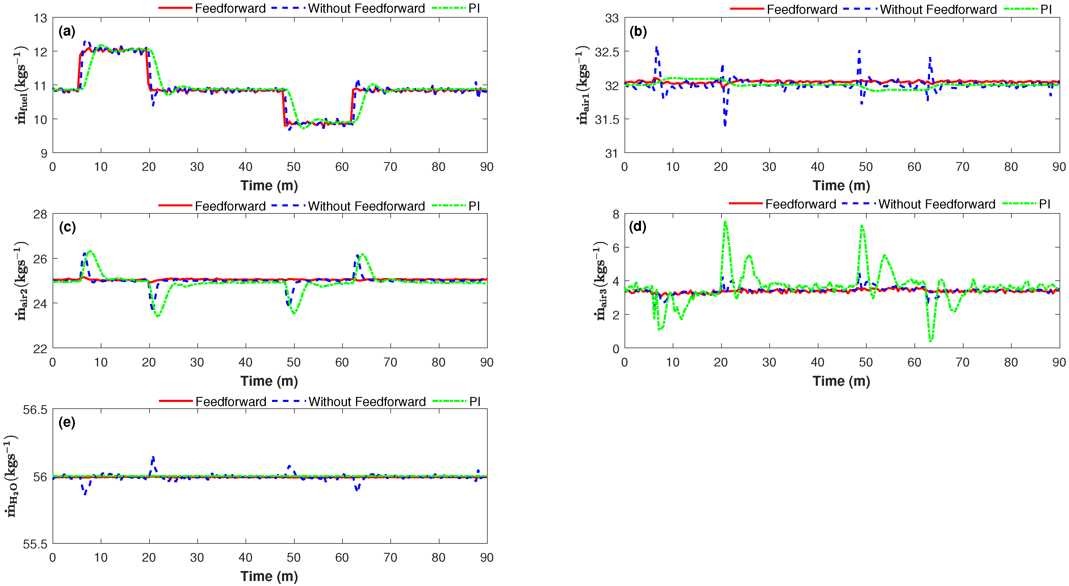
5.2. Control
Model Predictive Control
6. Conclusions
Author Contributions
Funding
Acknowledgments
Conflicts of Interest
References
- Van Caneghem, J.; Brems, A.; Lievens, P.; Block, C.; Billen, P.; Vermeulen, I.; Dewil, R.; Baeyens, J.; Vandecasteele, C. Fluidized bed waste incinerators: Design, operational and environmental issues. Prog. Energy Combust. Sci. 2012, 38, 551–582. [Google Scholar] [CrossRef]
- Basu, P.; Fraser, S.A. Circulating Fluidized Bed Boilers: Design, Operation and Maintenance; Springer International Publishing: Cham, Switzerland, 2015. [Google Scholar]
- Gungor, A. One dimensional numerical simulation of small scale CFB combustors. Energy Convers. Manag. 2009, 50, 711–722. [Google Scholar] [CrossRef]
- Basu, P. Combustion of coal in circulating fluidized-bed boilers: A review. Chem. Eng. Sci. 1999, 54, 5547–5557. [Google Scholar] [CrossRef]
- Huang, Y.; Turton, R.; Park, J.; Famouri, P.; Boyle, E.J. Dynamic model of the riser in circulating fluidized bed. Powder Technol. 2006, 163, 23–31. [Google Scholar] [CrossRef]
- Jiang, X.; Chen, D.; Ma, Z.; Yan, J. Models for the combustion of single solid fuel particles in fluidized beds: A review. Renew. Sustain. Energy Rev. 2017, 68, 410–431. [Google Scholar] [CrossRef]
- Huilin, L.; Guangbo, Z.; Rushan, B.; Yongjin, C.; Gidaspow, D. A coal combustion model for circulating fluidized bed boilers. Fuel 2000, 79, 165–172. [Google Scholar] [CrossRef]
- Pallarès, D.; Johnsson, F. Macroscopic modelling of fluid dynamics in large-scale circulating fluidized beds. Prog. Energy Combust. Sci. 2006, 32, 539–569. [Google Scholar] [CrossRef]
- Pugsley, T.S.; Berruti, F. A predictive hydrodynamic model for circulating fluidized bed risers. Powder Technol. 1996, 89, 57–69. [Google Scholar] [CrossRef]
- Davidson, J.F. Circulating fluidised bed hydrodynamics. Powder Technol. 2000, 113, 249–260. [Google Scholar] [CrossRef]
- Xu, G.; Gao, S. Necessary parameters for specifying the hydrodynamics of circulating fluidized bed risers—A review and reiteration. Powder Technol. 2003, 137, 63–76. [Google Scholar] [CrossRef]
- Wang, C.; Zhu, J.; Li, C.; Barghi, S. Detailed measurements of particle velocity and solids flux in a high density circulating fluidized bed riser. Chem. Eng. Sci. 2014, 114, 9–20. [Google Scholar] [CrossRef]
- Cai, R.; Zhang, H.; Zhang, M.; Yang, H.; Lyu, J.; Yue, G. Development and application of the design principle of fluidization state specification in CFB coal combustion. Fuel Process. Technol. 2018. [Google Scholar] [CrossRef]
- Wang, G.; Silva, R.B.; Azevedo, J.L.T.; Martins-Dias, S.; Costa, M. Evaluation of the combustion behaviour and ash characteristics of biomass waste derived fuels, pine and coal in a drop tube furnace. Fuel 2014, 117, 809–824. [Google Scholar] [CrossRef]
- Gungor, A. Two-dimensional biomass combustion modeling of CFB. Fuel 2008, 87, 1453–1468. [Google Scholar] [CrossRef]
- Saastamoinen, J. Simplified model for calculation of devolatilization in fluidized beds. Fuel 2006, 85, 2388–2395. [Google Scholar] [CrossRef]
- Liu, Z.S.; Peng, T.H.; Lin, C.L. Effects of bed material size distribution, operating conditions and agglomeration phenomenon on heavy metal emission in fluidized bed combustion process. Waste Manag. 2012, 32, 417–425. [Google Scholar] [CrossRef] [PubMed]
- Demirbas, A. Combustion characteristics of different biomass fuels. Prog. Energy Combust. Sci. 2004, 30, 219–230. [Google Scholar] [CrossRef]
- Krzywanski, J.; Rajczyk, R.; Bednarek, M.; Wesolowska, M.; Nowak, W. Gas emissions from a large scale circulating fluidized bed boilers burning lignite and biomass. Fuel Process. Technol. 2013, 116, 27–34. [Google Scholar] [CrossRef]
- Tang, Z.; Chen, X.; Liu, D.; Zhuang, Y.; Ye, M.; Sheng, H.; Xu, S. Experimental investigation of ash deposits on convection heating surfaces of a circulating fluidized bed municipal solid waste incinerator. J. Environ. Sci. 2016, 48, 1–10. [Google Scholar] [CrossRef] [PubMed]
- Lindberg, D.; Backman, R.; Chartrand, P.; Hupa, M. Towards a comprehensive thermodynamic database for ash-forming elements in biomass and waste combustion: Current situation and future developments. Fuel Process. Technol. 2013, 105, 129–141. [Google Scholar] [CrossRef]
- Pettersson, A.; Niklasson, F.; Moradian, F. Reduced bed temperature in a commercial waste to energy boiler—Impact on ash and deposit formation. Fuel Process. Technol. 2013, 105, 28–36. [Google Scholar] [CrossRef]
- Desroches-Ducarne, E.; Dolignier, J.; Marty, E.; Martin, G.; Delfosse, L. Modelling of gaseous pollutants emissions in circulating fluidized bed combustion of municipal refuse. Fuel 1998, 77, 1399–1410. [Google Scholar] [CrossRef]
- Alamoodi, N.; Daoutidis, P. Nonlinear control of coal-fired steam power plants. Control Eng. Pract. 2017, 60, 63–75. [Google Scholar] [CrossRef]
- Sun, L.; Li, D.; Lee, K.Y. Enhanced decentralized PI control for fluidized bed combustor via advanced disturbance observer. Control Eng. Pract. 2015, 42, 128–139. [Google Scholar] [CrossRef]
- Ji, G.; Huang, J.; Zhang, K.; Zhu, Y.; Lin, W.; Ji, T.; Zhou, S.; Yao, B. Identification and predictive control for a circulation fluidized bed boiler. Knowl.-Based Syst. 2013, 45, 62–75. [Google Scholar] [CrossRef]
- Hadavand, A.; Jalali, A.A.; Famouri, P. An innovative bed temperature-oriented modeling and robust control of a circulating fluidized bed combustor. Chem. Eng. J. 2008, 140, 497–508. [Google Scholar] [CrossRef]
- Havlena, V.; Findejs, J. Application of model predictive control to advanced combustion control. Control Eng. Pract. 2005, 13, 671–680. [Google Scholar] [CrossRef]
- Kortela, J.; Jämsä-Jounela, S.L. Modeling and model predictive control of the BioPower combined heat and power (CHP) plant. Int. J. Electr. Power Energy Syst. 2015, 65, 453–462. [Google Scholar] [CrossRef]
- Zimmerman, N.; Kyprianidis, K.; Lindberg, C.F. Agglomeration Detection in Circulating Fluidized Bed Boilers Using Refuse Derived Fuels. In Proceedings of the 2016 9th EUROSIM Congress on Modelling and Simulation, Oulu, Finland, 12–16 September 2016; pp. 123–128. [Google Scholar] [CrossRef]
- Hernandez-Atonal, F.D.; Ryu, C.; Sharifi, V.N.; Swithenbank, J. Combustion of refuse-derived fuel in a fluidised bed. Chem. Eng. Sci. 2007, 62, 627–635. [Google Scholar] [CrossRef]
- Xiao, X.; Yang, H.; Zhang, H.; Lu, J.; Yue, G. Research on Carbon Content in Fly Ash from Circulating Fluidized Bed Boilers. Energy Fuels 2005, 19, 1520–1525. [Google Scholar] [CrossRef]
- Lu, J.W.; Zhang, S.; Hai, J.; Lei, M. Status and perspectives of municipal solid waste incineration in China: A comparison with developed regions. Waste Manag. 2017, 69, 170–186. [Google Scholar] [CrossRef] [PubMed]
- ISWA. Waste-to-Energy State-of-the-Art-Report; Technical Report; ISWA: Copenhagen, Denmark, 2013. [Google Scholar]
- Yin, C.; Li, S. Advancing grate-firing for greater environmental impacts and efficiency for decentralized biomass/wastes combustion. Energy Procedia 2017, 120, 373–379. [Google Scholar] [CrossRef]
- Beyene, H.D.; Werkneh, A.A.; Ambaye, T.G. Current updates on waste to energy (WtE) technologies: A review. Renew. Energy Focus 2018, 24, 1–11. [Google Scholar] [CrossRef]
- Manfredi, S.; Tonini, D.; Christensen, T.H. Contribution of individual waste fractions to the environmental impacts from landfilling of municipal solid waste. Waste Manag. 2010, 30, 433–440. [Google Scholar] [CrossRef] [PubMed]
- Redemann, K.; Hartge, E.U.; Werther, J. Ash management in circulating fluidized bed combustors. Fuel 2008, 87, 3669–3680. [Google Scholar] [CrossRef]
- Sever Akdag, A.; Atımtay, A.; Sanin, F. Comparison of fuel value and combustion characteristics of two different RDF samples. Waste Manag. 2016, 47, 217–224. [Google Scholar] [CrossRef] [PubMed]
- Ripa, M.; Fiorentino, G.; Giani, H.; Clausen, A.; Ulgiati, S. Refuse recovered biomass fuel from municipal solid waste. A life cycle assessment. Appl. Energy 2016, 186, 211–225. [Google Scholar] [CrossRef]
- Malinauskaite, J.; Jouhara, H.; Czajczyńska, D.; Stanchev, P.; Katsou, E.; Rostkowski, P.; Thorne, R.J.; Colón, J.; Ponsá, S.; Al-Mansour, F.; et al. Municipal solid waste management and waste-to-energy in the context of a circular economy and energy recycling in Europe. Energy 2017, 141, 2013–2044. [Google Scholar] [CrossRef]
- Perrot, J.F.; Subiantoro, A. Municipal waste management strategy review and waste-to-energy potentials in New Zealand. Sustainability 2018, 10, 3114. [Google Scholar] [CrossRef]
- Sandberg, J. Fouling in Biomass Fired Boilers. Ph.D. Thesis, Mälardalen University, Västerås, Sweden, 2011. [Google Scholar]
- Yan, R.; Liang, D.T.; Laursen, K.; Li, Y.; Tsen, L.; Tay, J.H. Formation of bed agglomeration in a fluidized multi-waste incinerator. Fuel 2003, 82, 843–851. [Google Scholar] [CrossRef]
- Lin, W.; Dam-Johansen, K.; Frandsen, F. Agglomeration in bio-fuel fired fluidized bed combustors. Chem. Eng. J. 2003, 96, 171–185. [Google Scholar] [CrossRef]
- Skrivfars, B.J.; Zevenhoven, M.; Backman, R.; Ohman, M. Effect of Fuel Quality on the Bed Agglomeration Tendency in A Biomass Fired Fluidised Bed Boiler; Therm. Eng. Res. Assoc. Rep. No. Varmeforsk B8–803; Värmeforsk: Stockholm, Sweden, 2000. [Google Scholar]
- Gatternig, B. Predicting Agglomeration in Biomass Fired Fluidized Beds. Ph.D. Thesis, University of Erlangen–Nuremberg, Erlangen, Germany, 2015. [Google Scholar]
- Bartels, M.; Nijenhuis, J.; Kapteijn, F.; van Ommen, J.R. Case studies for selective agglomeration detection in fluidized beds: Application of a new screening methodology. Powder Technol. 2010, 203, 148–166. [Google Scholar] [CrossRef]
- Bartels, M.; Nijenhuis, J.; Kapteijn, F.; van Ommen, J.R. Detection of agglomeration and gradual particle size changes in circulating fluidized beds. Powder Technol. 2010, 202, 24–38. [Google Scholar] [CrossRef]
- Morris, J.D.; Daood, S.S.; Chilton, S.; Nimmo, W. Mechanisms and mitigation of agglomeration during fluidized bed combustion of biomass: A review. Fuel 2018. [Google Scholar] [CrossRef]
- Visser, H.J.M. The Influence of Fuel Composition on Agglomeration Behaviour in Fluidised-Bed Combustion; Duurzame Energy; ECN Biomass: Delft, The Netherland, 2004; p. 44. [Google Scholar]
- Vamvuka, D.; Zografos, D.; Alevizos, G. Control methods for mitigating biomass ash-related problems in fluidized beds. Bioresour. Technol. 2008, 99, 3534–3544. [Google Scholar] [CrossRef] [PubMed]
- Corcoran, A.; Knutsson, P.; Lind, F.; Thunman, H. Comparing the structural development of sand and rock ilmenite during long-term exposure in a biomass fired 12 MWthCFB-boiler. Fuel Process. Technol. 2018. [Google Scholar] [CrossRef]
- Ergun, S. Fluid flow through packed columns. Chem. Eng. Prog. 1952. [Google Scholar] [CrossRef]
- Fluidization Engineering, 2nd ed.; Butterworth Publishers: Waltham, MA, USA, 1991; p. 491.
- Kozak, S. State-of-the-art in control engineering. J. Electr. Syst. Inf. Technol. 2014, 1, 1–9. [Google Scholar] [CrossRef]
- Sultana, W.R.; Sahoo, S.K.; Sukchai, S.; Yamuna, S.; Venkatesh, D. A review on state of art development of model predictive control for renewable energy applications. Renew. Sustain. Energy Rev. 2017, 76, 391–406. [Google Scholar] [CrossRef]
- Garg, A.; Corbett, B.; Mhaskar, P.; Hu, G.; Flores-Cerrillo, J. Subspace-based model identification of a hydrogen plant startup dynamics. Comput. Chem. Eng. 2017, 106, 183–190. [Google Scholar] [CrossRef]
- Khani, F.; Haeri, M. Robust model predictive control of nonlinear processes represented by Wiener or Hammerstein models. Chem. Eng. Sci. 2015, 129, 223–231. [Google Scholar] [CrossRef]
- Al Seyab, R.; Cao, Y. Nonlinear model predictive control for the ALSTOM gasifier. J. Process Control 2006, 16, 795–808. [Google Scholar] [CrossRef]
- Van Overschee, P.; De Moor, B. Subspace Identification for Linear Systems; Springer: Boston, MA, USA, 1996. [Google Scholar]


| Temperature (C) | Mass Flow Rate (kg s) | |
|---|---|---|
| fuel | - | x |
| primary air | x | x |
| secondary air | x | x |
| flue gas recirculation | x | x |
| feed water | x | x |
| MO/CV | FFMPC | NFFMPC | PI |
|---|---|---|---|
| () | 0.222 | 0.788 | 1.0877 |
| () | 0.265 | 1.336 | 4.331 |
| () | 0.015 | 0.071 | 0.298 |
| () | 0.0039 | 0.074 | 0.029 |
| ( ) | 0.0006 | 0.0006 | 0.0006 |
| ( ) | 0.611 | 0.626 | 0.596 |
| ( ) | 0.016 | 0.105 | 0.0461 |
| ( ) | 0.026 | 0.259 | 0.433 |
| ( ) | 0.103 | 0.217 | 0.974 |
| ( ) | 0.0016 | 0.026 | 0.0002 |
© 2018 by the authors. Licensee MDPI, Basel, Switzerland. This article is an open access article distributed under the terms and conditions of the Creative Commons Attribution (CC BY) license (http://creativecommons.org/licenses/by/4.0/).
Share and Cite
Zimmerman, N.; Kyprianidis, K.; Lindberg, C.-F. Waste Fuel Combustion: Dynamic Modeling and Control. Processes 2018, 6, 222. https://doi.org/10.3390/pr6110222
Zimmerman N, Kyprianidis K, Lindberg C-F. Waste Fuel Combustion: Dynamic Modeling and Control. Processes. 2018; 6(11):222. https://doi.org/10.3390/pr6110222
Chicago/Turabian StyleZimmerman, Nathan, Konstantinos Kyprianidis, and Carl-Fredrik Lindberg. 2018. "Waste Fuel Combustion: Dynamic Modeling and Control" Processes 6, no. 11: 222. https://doi.org/10.3390/pr6110222
APA StyleZimmerman, N., Kyprianidis, K., & Lindberg, C.-F. (2018). Waste Fuel Combustion: Dynamic Modeling and Control. Processes, 6(11), 222. https://doi.org/10.3390/pr6110222