Simulation of High Pressure Separator Used in Crude Oil Processing

Abstract

The aim of this research was to simulate a high-pressure (HP) separator in order to investigate the effect of changing separator operating conditions on product properties. In this study, the results obtained using the CHEMCAD simulation software package were compared with those obtained using the UniSim software package. The simulation results were comparable with industrial data. A sensitivity study was conducted by changing the gas stream properties, such as temperature, pressure, and flow rate, in order to investigate and optimize the process. The results showed that increasing the separator inlet pressure from 30 to 80 bar decreased the outlet gas flow rate from 1202 to 871.15 kmol/h. Also, the methane mole fraction increased from 0.69 to 0.74; however, the preheater heating duty was increased from 8.71 to 11.48 GJ/h. The simulation results showed that increasing the temperature of the separator feed stream from 43 to 83 °C increased the flow rate of the outlet gas stream from 871.15 to 1142.98 kmol/h. However, this temperature change reduced the methane concentration in the gas product and decreased the heating duty of the heat exchanger. Finally, the study demonstrated that there is no effect of increasing the inlet feed flow rate on the produced methane gas concentration.

1. Introduction

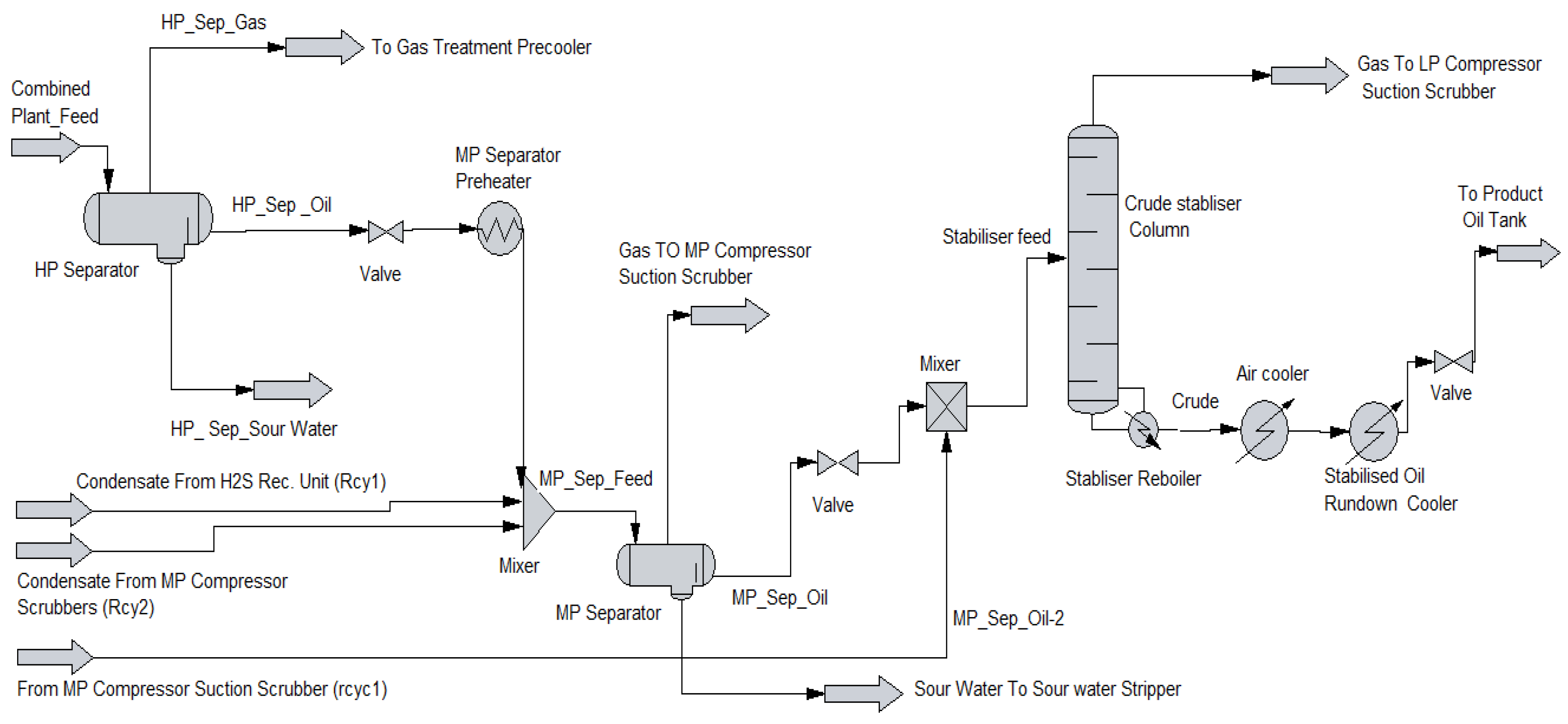
1.1. Separation Vessel Used in Crude Oil Processing

Crude oil processing involves the separation of oil from other substances present, i.e., gas and water. Having these three fluids as separated streams makes any further technical treatment easier, since processing single-phase fluids is less technically challenging than dealing with multi-phase fluids. In addition, it is more economical, since the movement of the single phases requires less energy. Additionally, the removal of produced water, which is corrosive, reduces the cost of downstream processing [1]. A pressure vessel with an inbuilt gravity separator is used for the separation process of the multi-phase flow. The classification of such separators can be defined either by their configurations (i.e., vertical, horizontal, or spherical separators) or by their separation function (e.g., separation of phases). In addition, the operating condition (pressure) of the vessels can be used to categorize them; hence, high-, medium- and low-pressure separators are all different types of separators [2,3]. Vertical and horizontal separators are commonly used to separate three-phase streams. Details of the separator function and technical considerations can be found in the literature (Abdel-Aal et al. [3]; N. Lieberman and E. Lieberman [4]; Seader et al. [5]).

The main step in the processing of upstream oil and gas is the separation into target fraction flows (i.e., splitting this stream into crude oil, gas and water). Therefore, a three-stage separation process (HP, medium pressure (MP) and low pressure (LP) separators) is utilized, because if only one separator is used, it will create a flash process that vaporizes the hydrocarbons, which will have negative safety implications. The reason for this flash vaporization is the significant reduction in pressure that occurs in the separation process. Thus, using a three-stage separation process controls component volatilization during the process. The HP and MP separators are of the gravity type, while the LP separator works by reducing the pressure to atmospheric pressure. Additionally, a choke is used to reduce the oil-well pressure to the HP separator pressure (3–11.5 MPa). The operating temperature of this first stage separation process is approximately 100 to 150 °C. Consequently, the gas bubbles out, water settles at the bottom of the vessel, and the oil forms in a layer on top of the water. The HP separator achieves a reduction in the stream water content from 40% to about 5%. The MP separator operates at a pressure of 0.7–3.5 MPa and at a temperature of less than 100 °C. Also, it may receive additional product from the low-pressure manifold, and it reduces the water content to less than 2%. A heat exchanger (preheater) can be placed between the HP and MP separators to reheat the stream. A LP separator with an operating pressure of up to 0.7 MPa also has a final stage separator incorporated into it, which is known as a flash drum; it allows the least volatile gas components to boil and separate from the oil. Therefore, a LP separator is a two-phase separator. These separators have pressure and level control systems [6,7].

1.2. Simulation Model

Equations of state (EOS) are commonly used in chemical engineering design, and particularly, in studying the phase equilibria of fluid mixtures. The Peng-Robinson (PR) [8] and the Soave-Redlich-Kwong (SRK) model [9] are modified forms of the van der Walls equation [10]. Equations of state models are highly reliable in predicting the properties of hydrocarbon-based fluids. Moreover, other models, which are known as thermodynamics packages, are used to calculate the equilibrium constant. Thus, the Peng-Robinson (PR) model is widely used to predict a wide range of K-values for medium-high pressure hydrocarbons systems (e.g., for oil, gas, and petrochemicals). Additionally, it can efficiently model single, dual, and three-phase systems. Furthermore, the PR model is considered to be the best thermodynamics package for cryogenic fluids [11,12]. The high accuracy of this model in representing the relationship between different parameters’ in the system, such as pressure, composition, and temperature, make it a widely-used method in industry. Additionally, this model is preferred for over the Soave-Redlich-Kwong equation (SRK), because of its superior performance. Aside from this, the properties at critical point and the acentric factor are needed for the generalized parameters [11]. The prediction of liquid density and vapor pressure can be calculated using the PR formulas that incorporate the modifications proposed by Peng and Robinson into the PR model [8]. To extend its application, various modifications were implemented. However, discussing these attempts is beyond the scope of this paper; they can be found in (Sengers et al. [13]; Valderrama [14]).

In most crude oil and gas applications, a mixture of fluids is present, for which a similar behavior can be assumed for both a mixture and a pure component. Therefore, it is possible to mathematically express the EOS for both identically. However, the calculation of parameters cannot be done in the same way [15]. Therefore, mixing rules that depend on the parameters of pure components are usually implemented. By utilizing the equations of state in the PR model, the constants of the fugacity and compressibility of a mixture of the phases (e.g., gas and liquid) can be found. Since the Binary interaction parameters (BIP) are available for most hydrocarbons and for gases that are not condensable, providing this data is not required, although it is possible to supply such data or to modify them in the CHEMCAD simulation software package (Chemstations Inc., Houston, TX, USA) [11,16].

Non-polar hydrocarbons form a fluid that is commonly found in the oil and gas industry. For such fluids, EOS can model the simulation problem. For example, the SRK and PR models are used to analyse hydrocarbon systems at a pressure above one atmosphere [17,18,19]. Additionally, representing two phases with a model is needed. However, the pressure has an influence on the liquid phase in many applications [17]. Furthermore, the gas phase deviates from the ideal case above atmospheric pressure, which requires the use of EOS for the gas phase. Similarly, the pressure affects the coefficient of activity of the liquid phase. The mixture composition, the system pressure value, and the available data determine the selection of the best model to describe systems in equilibrium [20].

1.3. Simulation and Model Selection

The simulation of chemical processes is represented through a mathematical model. This model, that involves linear, non-linear and differential algebraic equations, provides material and energy balances that are associated with phase equilibrium and the kinetics of the system, and it can predict the process plant behaviour. Accordingly, a process flow diagram, which is created using a simulation software package such as CHEMCAD, connects the unit operations of a plant with their operating conditions. The simulation software package solves the equations of the units individually, and it uses the results of a unit in the calculation of the following equipment. Nevertheless, if a process contains recycle streams, a tear stream must be taken because of the necessity of using some parameter values in the initialization of the process [21]. Dependent and independent variables have to be identified before running any optimization for the process (i.e., the parameters are related by an objective function that defines the interaction between the variables). The main optimization goal is to minimize the consumption of energy and the cost of the process operation. Because of the potential change in the feed composition, as well as a potential change in a plant unit operations configuration and environmental conditions, it is obvious that a plant does not work under its design conditions. Therefore, the simulation software package allows the prediction of the effect of operating condition changes on the other process parameter [21].

The PR package is implemented in hydrocarbon processes. A group contribution is integrated in the PR model to estimate BIP. Therefore, it is used for all known real natural gas mixture constituents. There is not a general rule that is used for selecting the model. However, Figure 1 presents a procedure for selecting a suitable model. Nevertheless, adequate measured data is required for the correct selection of a model [20].

1.4. Research Aim and Outcome

The novelty of this research is in the simulation and optimization of an existing plant separator unit and in the comparison between the results obtained from the CHEMCAD and the provided data of UniSim simulation software package (Honeywell Inc, Morris Plains, NJ, USA). Also, the study introduces an approach of relating the results of a parameter study (e.g., temperature and pressure) with the gas phase envelope diagram. Therefore, a potential optimum operating condition of a HP separator can be located on this diagram. Moreover, this point can be compared with a current used operating condition. In consequence, the produced gas will be processed at the phase envelope maximum temperature to prevent the formation of the liquid phase that is caused by the change of the gas state, i.e., from a gas phase to the two-phase region (liquid + gas), when the pressure drops in the pipeline. Therefore, the aim of this work is to simulate a real crude oil HP separator. It includes studying the effect of changing different parameters of the feed stream, such as temperature, pressure, and flow rate, on the separation unit operation (HP-separator). Running such a sensitivity study allows us to predict the HP separator’s capacity and its optimum operating conditions. Therefore, it improves the ability to analyze the effect of changing the operating conditions on the quantity and quality of the product. Furthermore, it shows the potential of increasing plant capacity. Consequently, since the inlet stream is a hydrocarbon system at 43 °C and 80 bar, the PR model was used as the thermodynamic package in the simulation. In this study, several attempts were made with other EOS (e.g., SRK), to simulate the whole process. However, only the PR model gave the best results that match the real measured values obtained from industrial data. This finding shows the potential of following the model selection procedure that is shown in Figure 1. Additionally, Figure 1 demonstrates that the PR model has been used for a system that is similar to the system studied in this work (i.e., hydrocarbon system).

2. Materials and Methods

2.1. Process Simulation

Although this work focused on the simulation of a HP separator unit, a process flow diagram (PFD) of a complete industrial crude oil processing plant was created, since this is required in order to run the flow sheet in the simulation software package. This simulation flow sheet and the process description were created according to an industrial process operational manual (the company name is not mentioned in this paper for confidentiality reasons). Moreover, the flow sheet must converge before completing any further unit operation simulations. Therefore, the flow sheet was created by using the CHEMCAD simulation software package, which successfully converged, as shown in Figure 2. As soon as the crude oil stream enters a three-phase HP separator, a reduction in the gas flow rate occurs, which enables the start of the separation process. A vertical coarse screen, a weir, and a vertical demister are the main components in the HP separator. The demister function is to separate the liquid droplets that are carried with the vapor. This HP separator works at pressure of 7900 kPa, while its temperature varies between 20–45 °C, in order to operate with different feed temperatures.

Overhead gas, sour water, and oil are the three product streams from the HP separator. Hence, the gas is collected from the top of the vessel, while the sour water is obtained from the bottom. This allows the oil to float over the water and to move over the weir plate; however, these oil streams still have gases and water dissolved in them. Therefore, it is sent to a medium pressure (MP) separator after passing it through a preheater, which is a heat exchanger with two heat exchange circuits, in order to heat the stream to the temperature range of 65–77 °C that is required by the other MP separator. Valves are used to reduce the pressure of the streams according to the design requirements.

To increase the efficiency of separation in the MP separator, it is fitted with a Schoepentoeter. Additionally, the installation of a bottom boot leg is necessary to accumulate any sour water that is sent to the stripper for further treatment. Similar to the HP separator, the gas is obtained from the top of the vessel. However, the produced oil is processed in the crude stabilizer column that works at a pressure of 400 kPa. The column was provided with its required heat by a kettle re-boiler, which is horizontally orientated. This re-boiler normally has U-shaped tubes inside it. This column is used to separate components that are volatile from the oil. Another role of this re-boiler is to maintain the required temperature that is necessary for sustaining the desired vapor pressure value. The oil product, collected from the bottom of the column, passes through two stages of cooling (air cooler and rundown cooler) before it goes to the oil tank. The gas top product is compressed in a low-pressure compressor to enable it to be mixed with the vapor of the MP separator. A compressor is used to elevate the pressure of this outlet stream before it is connected with the gas stream that comes from another HP separator. Finally, the gas stream is directed to the treatment process for the gas.

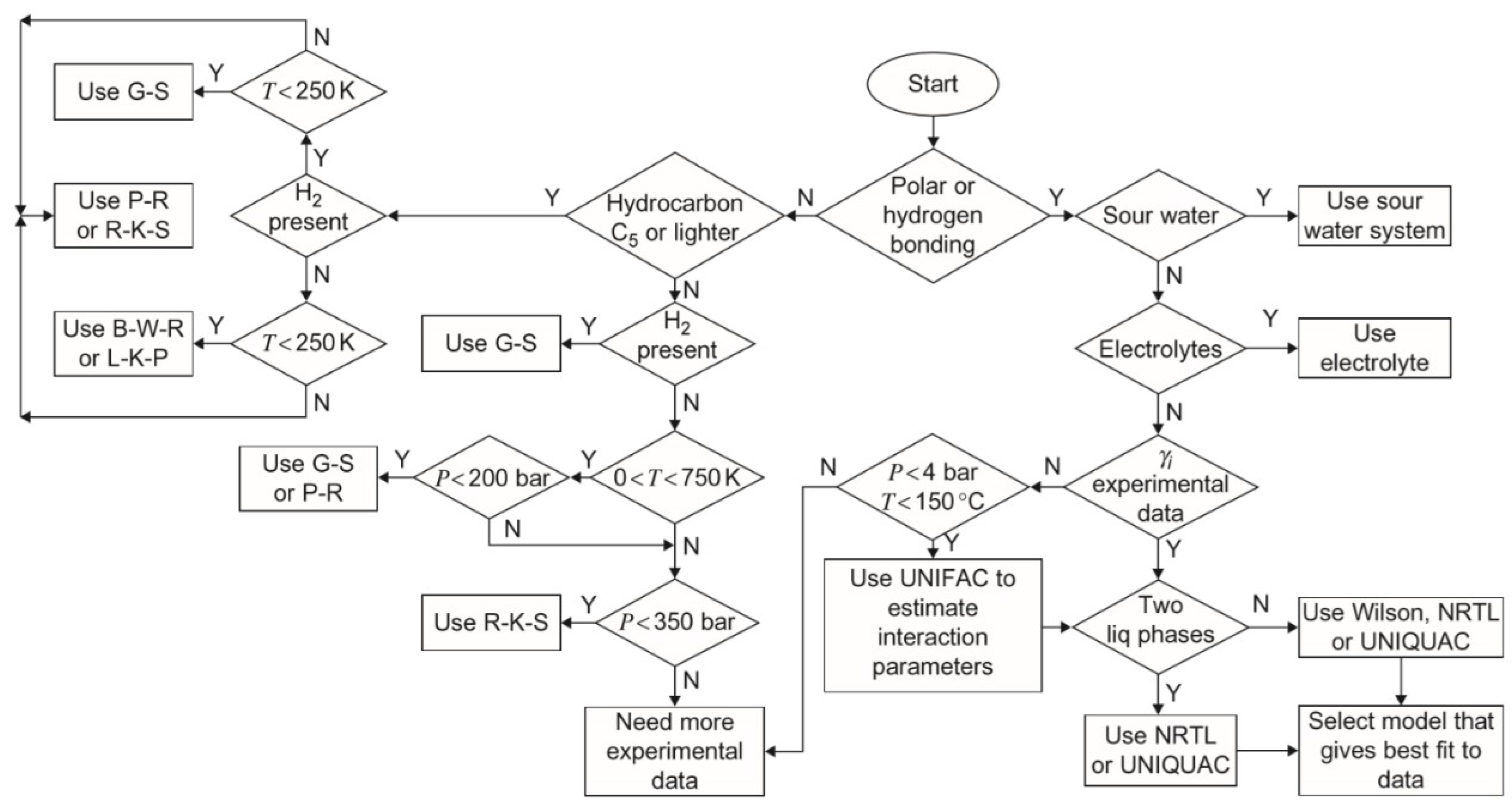
2.2. Thermodynamics Package

The following Peng-Robinson formula, Equation (1), was used in this simulation. It is crucial to obtain a high accuracy for the calculated compressibility-factor (Z) that appears in Equation (2). Equation (3) is used to calculate the fugacity coefficient that is necessary for the equilibrium constant, K value, calculation [8,11,16]. The model is a thermodynamics package that is used to calculate the K value accurately, since it is used for the whole plant simulation. The accurate model enables the calculation of the stream and unit operations properties, by using other formulas that are integrated into the software.

$$P=\frac{RT}{V-b}-\frac{a}{\left(V^2+Vb\right)+b\left(V-b\right)}$$

(1)

where

$$b={\displaystyle \sum }_i^n{x}_i{b}_i$$

$$b_i=0.077796\frac{R{T}_{c_i}}{P_{C_i}}$$

$$a={\displaystyle \sum }_i^n{\displaystyle \sum }_l^n{x}_i{x}_l\sqrt{\left(a_i{a}_l\right)}\left(1-k_{il}\right)$$

$$a_i={\alpha }_i a{c}_i$$

$$a{c}_i=0.457235\frac{{(R{T}_{C_i})}^2}{P_{C_i}}$$

$$\sqrt{{\alpha }_i}=m_i\left(1-\sqrt{T_{r_i}}\right)+1$$

$$T_{r_i}=\frac{T_i}{T_{C_i}}$$

$$m_i=0.37464+\left(1.54226 {\omega }_i\right)-\left(0.26992 {\omega }_i^2\right)$$

where P is the total pressure (Pa), $R$ is the universal gas constant (J·mol⁻¹·K), $T$ is the absolute temperature (K), V is the volume (m³), $b$ is the repulsive parameter in equation of state (m³·mol⁻¹), $a$ is the attractive parameter in cubic equations of state (J·m³·mol⁻²), $x_i$ is the mole fraction of component i in the liquid phase, $b_i$ is an empirical coefficient selected by the simulator, $T_{C_i}$ is the temperature of component i at critical point (K), $P_{C_i}$ is the pressure of component i at critical point (Pa), $k_{il}$ is the binary interaction parameter in cubic equations of state, $a_i$ is an empirical coefficient selected by the simulator, ${\alpha }_i$ is an empirical coefficient selected by the simulator, $a{c}_i$ is an empirical coefficient selected by the simulator, $T_{r_i}$ is the reduced temperature (dimensionless), $m_i$ is an empirical coefficient selected by the simulator, and $w$ is the acentric factor.

$$Z^3-Z^2+B{Z}^2+(AZ-2BZ-3B^{2}Z)+AB-B^2-B^3=0$$

(2)

where Z is the compressibility factor. Moreover, A and $B$ are empirical coefficients selected by the simulator

$$\ln {\varphi }_1=-\ln \left(Z-B\right)+\left(B_{i}Z-B_i\right)-\frac{A}{2.82843\times B\times \left[A_i-B_i\right]}\times \ln [\frac{\left(Z+2.4142B\right)}{\left(Z-0.4142B\right)}]$$

(3)

where

$$\mathit{A}=\frac{\mathit{a}\mathit{P}}{{(\mathit{R}\mathit{T})}^{\mathbf{2}}}$$

$$\mathit{B}=\frac{\mathit{b}\mathit{P}}{(\mathit{R}\mathit{T})}$$

$${\mathit{B}}_{\mathit{i}}=\frac{{\mathit{b}}_{\mathit{i}}}{\mathit{b}}$$

$${\mathit{A}}_{\mathit{i}}=\frac{\mathbf{1}}{\mathit{a}}\times [\mathbf{2}\times {\mathit{a}}_{\mathit{i}}^{\mathbf{0.5}}\sum {\mathit{x}}_{\mathit{i}}\times {\mathit{a}}_{\mathit{j}}^{\mathbf{0.5}}\times \left(\mathbf{1}-{\mathit{k}}_{\mathit{i}\mathit{j}}\right)]$$

$${\mathit{K}}_{\mathit{i}}=\frac{{\mathit{y}}_{\mathit{i}}}{{\mathit{x}}_{\mathit{i}}}=\frac{{\mathit{\Phi }}_{\mathit{i}\mathit{l}}}{{\mathit{\Phi }}_{\mathit{i}\mathit{v}}}$$

where A, $A_{i ,} B$, and $B_i$ are empirical coefficients selected by the simulator. Additionally, ${\Phi }_i$ is the fugacity coefficient of component i, ${\Phi }_{il}$ is the fugacity coefficient of component i in liquid phase, ${\Phi }_{iv}$ is the fugacity coefficient of component i in vapor phase, $K_i$ is the K-value of component, and $y_i$ is the mole fraction of component i in the vapor phase.

2.3. Simulation Conditions

The three-phase HP separator unit was simulated using the CHEMCAD and UniSim simulation software packages. The composition of the inlet feed, which is illustrated in Figure 2 as a combined plant feed, can be found in

Table 1. HP separator feed composition.

Component	Chemical Formula	Mass Flow Rate (kg/h)
Hydrogen Sulfide	H2S	854.1820
Carbon Dioxide	CO2	2041.8970
Nitrogen	N2	399.9500
Methane	CH4	13,924.100
Ethane	C2H6	6194.2178
Propane	C3H8	6045.8480
I-Butane	C4H10	889.7230
N-Butane	C4H10	3771.3100
I-Pentane	C5H12	1349.6700
N-Pentane	C5H12	2748.3030
N-Hexane	C6H14	3769.9010
Heptane	C7H16	3795.1810
Octane	C8H18	4069.6010
Nonane	C9H20	3773.9570
Decane	C10H22	3366.5690
Undecane	C11H24	3173.9910
Dodecane	C12H26	2725.6790
Tridecane	C13H28	2585.4040
Tetradecane	C14H30	2321.1870
Pentadecane	C15H32	2065.0300
Hexadecane	C16H34	1831.2710
Heptadecane	C17H36	1717.1020
Octadecane	C18H38	1532.6370
Nonadecane	C19H40	1570.9020
Water	H2O	987.6000

. The operating conditions, simulation, and design parameters of the HP separator can be found in

Table 2. Operating conditions and design parameters of the HP separator.

Parameter	Design (Range)	Unit Operating Conditions (Design)	Unit Operating Conditions (Data)	Simulation Data Input
Temperature (°C)	−10 to 80	20–45	43	43
Pressure (bar)	Up to 92	78–83	80	80
Feed flow rate (kmol/h)	-	1215.6480	1800.5150	1800.5150

. The design parameters were determined according to existing plant data. The PR model was used as the thermodynamic package in this simulation.

2.4. Sensitivity Study

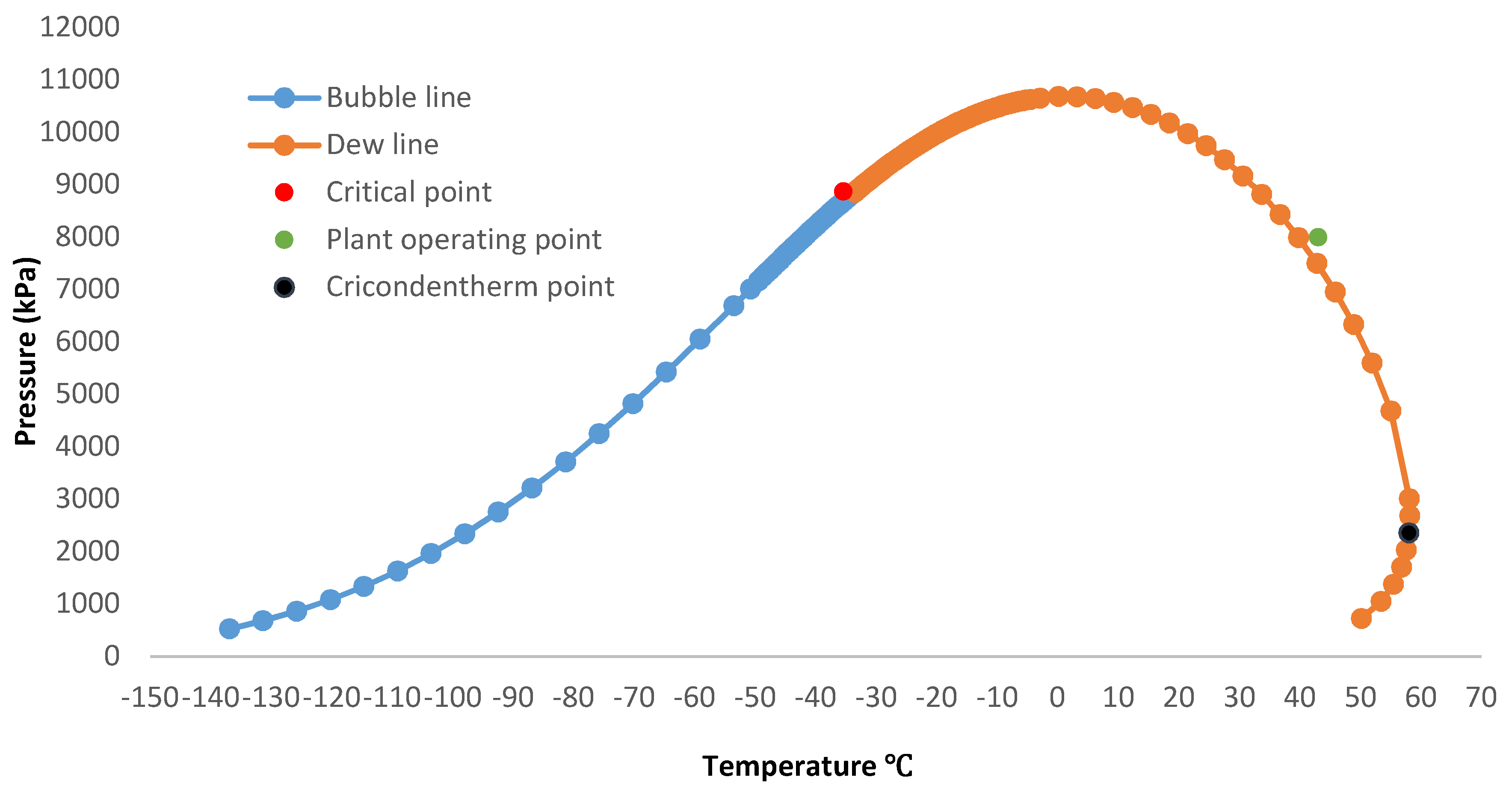
A sensitivity study was performed to investigate the effect of varying the feed stream properties, such as temperature, pressure, and flow rate, on the heat required for the preheater and on the gas production quality and quantity. Therefore, this study will indicate the range of operating conditions.

2.5. Phase Envelope

Michelsen [22] described the calculation of the phase envelope. However, to determine the phase of the obtained gas stream, CHEMCAD was used to generate the phase envelope of the gas stream. The PR model refers to the thermodynamics package that was used in the creation of the critical point, and the dew and bubble lines of the gas phase envelope. The operating condition of the plant was located on the phase envelope diagram as well.

3. Results and Discussion

The simulation results of all streams were comparable, as shown in

Table 3. Comparison of the results obtained for the HP separator parameters (normalized values).

Inlet Feed Components	Normalized Inlet Feed Mole Fraction (Provided Data and Simulation)	Normalized Outlet Gas Mole Fraction (Provided Data)	Normalized Outlet Gas Mole Fraction (Simulation)	Normalized Outlet Liquid Phase Stream Product (Provided Data)	Normalized Outlet Liquid Phase Stream Product (Simulation)
H2S	0.0143	0.0121	0.0122	0.0175	0.0174
CO2	0.0264	0.0316	0.0323	0.0224	0.0217
Nitrogen	0.0081	0.0139	0.0139	0.0024	0.0023
Methane	0.4938	0.7411	0.7560	0.2577	0.2405
Ethane	0.1172	0.1204	0.1126	0.1212	0.1297
Propane	0.0780	0.0508	0.0463	0.1125	0.1175
i-Butane	0.0087	0.0037	0.0034	0.0147	0.0151
n-Butane	0.0369	0.0133	0.0120	0.0649	0.0663
i-Pentane	0.0106	0.0023	0.0022	0.0203	0.0205
n-Pentane	0.0217	0.0041	0.0037	0.0421	0.0426
n-Hexane	0.0249	0.0024	0.0021	0.0509	0.0512
Heptanes	0.0215	0.0017	0.0009	0.0444	0.0453
Octanes	0.0203	0.0007	0.0004	0.0428	0.0431
Nonanes	0.0167	0.0003	0.0002	0.0356	0.0358
Decanes	0.0135	0.0001	0.0001	0.0288	0.0289
Undecanes	0.0116	0.0001	0.0000	0.0247	0.0248
Dodecanes	0.0091	0.0000	0.0000	0.0195	0.0196
Tridecanes	0.0080	0.0000	0.0000	0.0171	0.0172
Tetradecane	0.0067	0.0000	0.0000	0.0143	0.0143
Pentadecans	0.0055	0.0000	0.0000	0.0119	0.0119
Hexadecanes	0.0046	0.0000	0.0000	0.0099	0.0099
Heptadecane	0.0041	0.0000	0.0000	0.0087	0.0087
Octadecanes	0.0034	0.0000	0.0000	0.0074	0.0074
Nonadecanes	0.0033	0.0000	0.0000	0.0071	0.0072
H2O	0.0312	0.0015	0.0015	0.0012	0.0011
Total	1	1	1	1	1

. Therefore, a further study was conducted by changing the operating conditions of the HP separator, in order to investigate their effect on the separation process. Hence, the outlet gas flow rate, product stream methane composition, and the heating duty of the preheater, were evaluated by varying the feed stream parameters (i.e., the temperature and pressure) while maintaining a constant flow rate. The study was conducted using the CHEMCAD software package, and the results were compared with those obtained by using the UniSim software package. It can be seen from the data presented in the following figures that the results produced by the two different simulation software packages were slightly different, which will be discussed in the following sections.

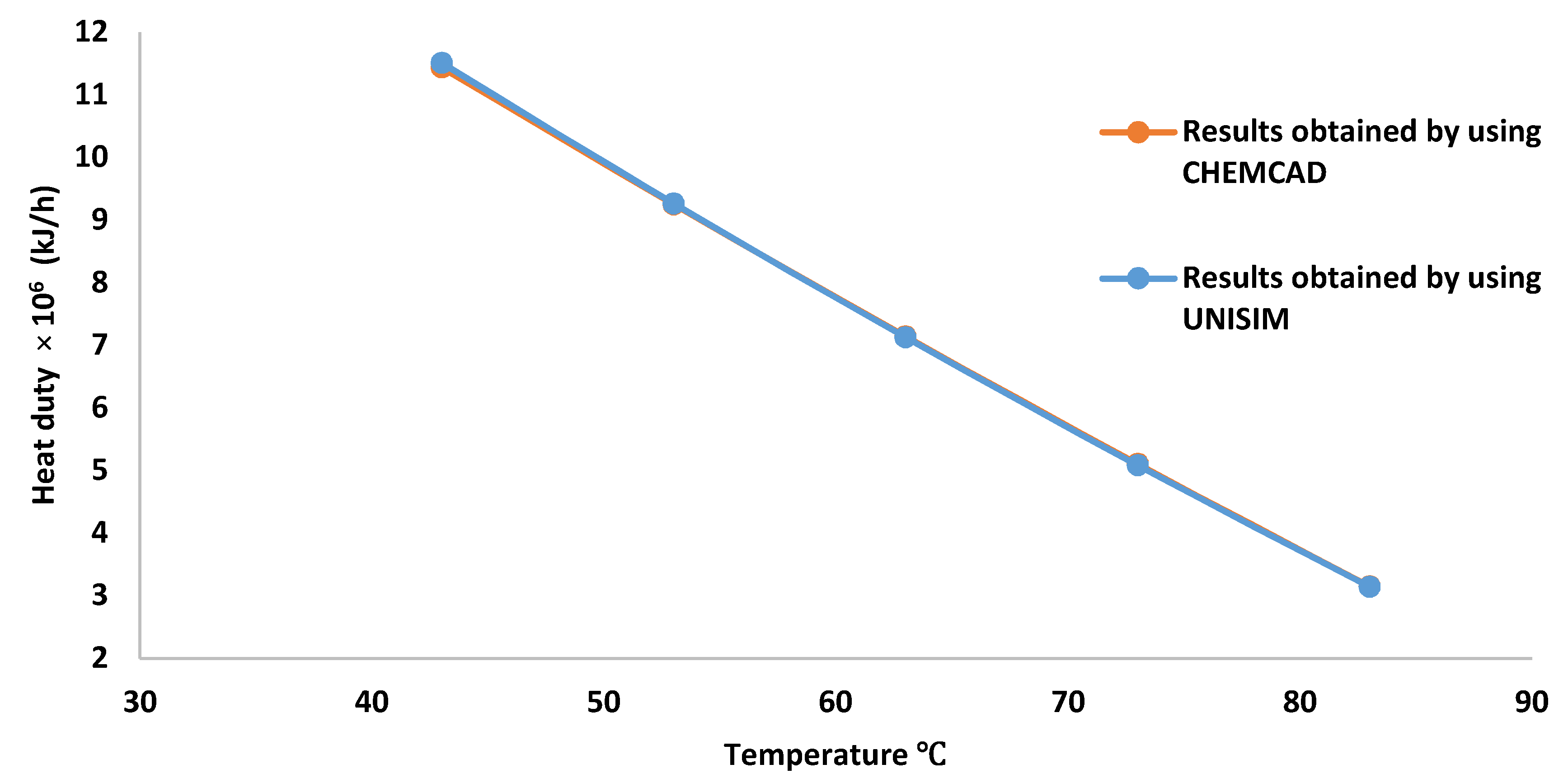
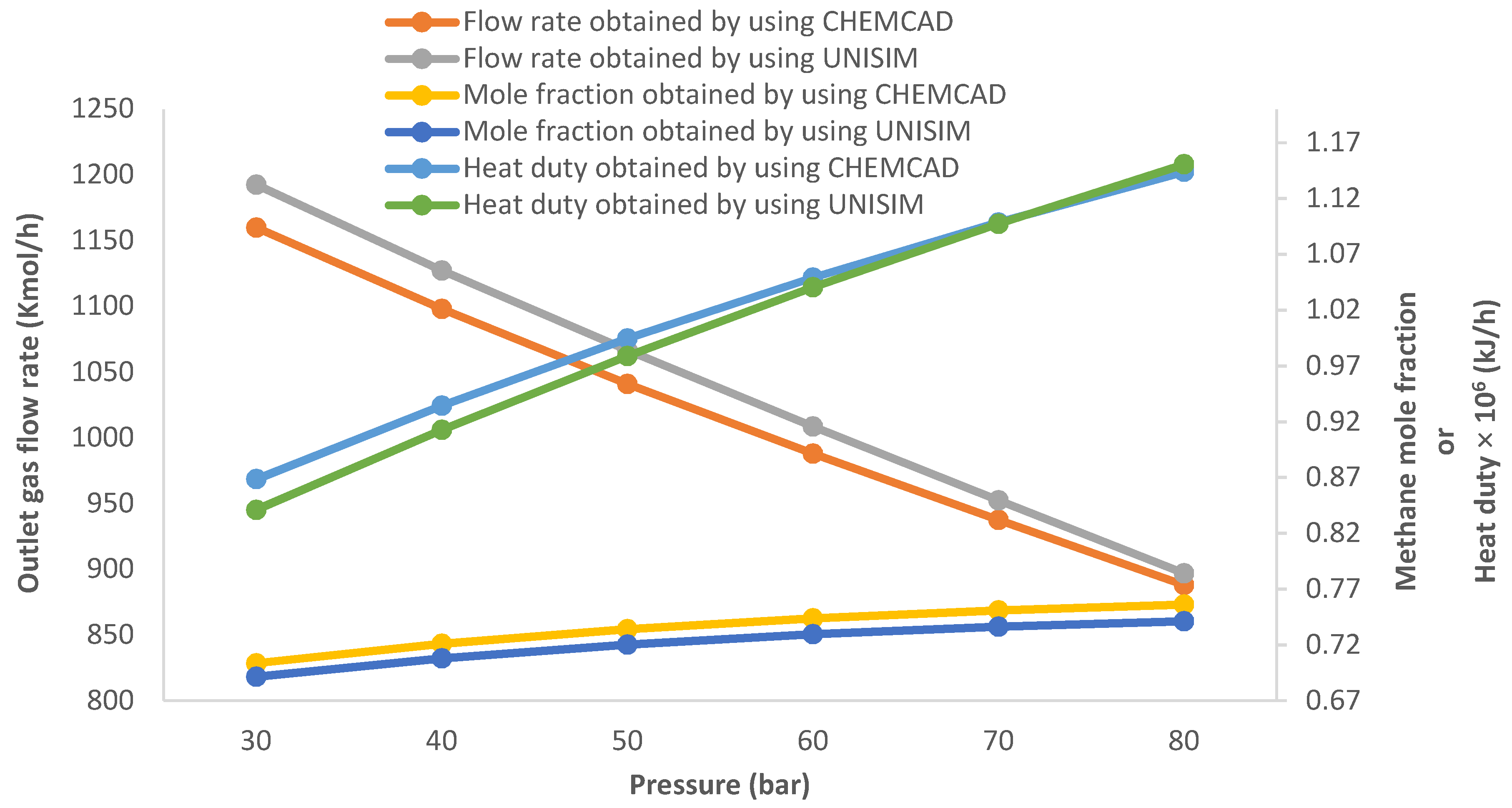
3.1. Effect of Changing the Pressure of the HP Sparator on the Gas Flow Rate, Methane Concentration and Preheater Heating Duty

The results demonstrate that changing the feed stream pressure from 30 to 80 bar decreases the outlet gas flow rate of the HP separator from 1160 to 888 kmol/h and from 1192.72 to 896.94 kmol/h, in the CHEMCAD and UniSim software package, respectively. This agrees with the fact that an increase in the pressure causes a reduction in the boiling point of a substance. This is a result of an increase of the vapor pressure. As a consequence, less vapor can be created, which means that the vapor flow rate will be reduced. However, methane mole fraction was slightly increased from 0.704 to 0.756 in CHEMCAD and from 0.6915–0.7412 in UniSim, which is a result of the condensation of other components, since the operating pressure approached its vapor pressure at the HP separator temperature. In terms of the heating duty of the MP preheater, a significant change was found: from 8.705 to 11.48 GJ/h (CHEMCAD) and from 8.411–11.506 GJ/h (UniSim). Increasing the pressure increased the volume of the obtained liquid hydrocarbon because of the drop in the amount of evaporated hydrocarbons. These results are shown in Figure 3.

3.2. High Pressure Separator Temperature Effect on the Gas Flow Rate, Methane Concentration and Preheater Heating Duty

The results of varying the inlet temperature of the HP separator from 43 to 83 °C on the gas production and methane mole fraction in the separator, in both simulators (CHEMCAD and UniSim), are shown in

Table 4. Temperature effect on flow rate and methane mole fraction (CHEMCAD).

Separator Temperature (°C)	Gas Flow Rate (kmol/h)	Methane Mole Fraction
43	871.1500	0.7560
53	937.7800	0.7399
63	1004.9700	0.7241
73	1073.1800	0.7086
83	1142.9800	0.6934

and

Table 5. Temperature effect on flow rate and mole fraction of methane (UniSim).

Separator Temperature (°C)	Gas Flow Rate (kmol/h)	Methane Mole Fraction
43	896.9400	0.7412
53	950.5100	0.7248
63	1000.6800	0.7089
73	1048.3200	0.6935
83	1094.2600	0.6783

respectively. The produced gas flow rate rises from 871.15 to 1142.98 kmol/h and from 896.94 to 1094.26 kmol/h in CHEMCAD and UniSim, respectively. These increases in gas flow rates are a result of the vaporization of more hydrocarbons, since they reach their saturation temperature in the separator. As a consequence, raising the inlet temperature can cause a change in the outlet vapor mass flow rate that comes from the HP separator. Nevertheless, a very slight decrease in the gas stream methane concentration occurred: from 0.75 to 0.69 (CHEMCAD) and from 0.7412 to 0.678304 (UniSim).

In contrast to the pressure effect, the required heating duty of the preheater dropped because its feed stream, which is entering the preheater, was already hot, and thus, had a lower quantity of liquid hydrocarbons. Therefore, it required less energy to achieve the required process temperature. Figure 4 illustrates the reduction in the heating duty, from 11.5 to 3.2 GJ/h, which was obtained in both simulation software packages. However, it should be remembered that operating the HP separator at higher temperatures requires additional energy in the form of heating. Thus, an optimization of the process is required.

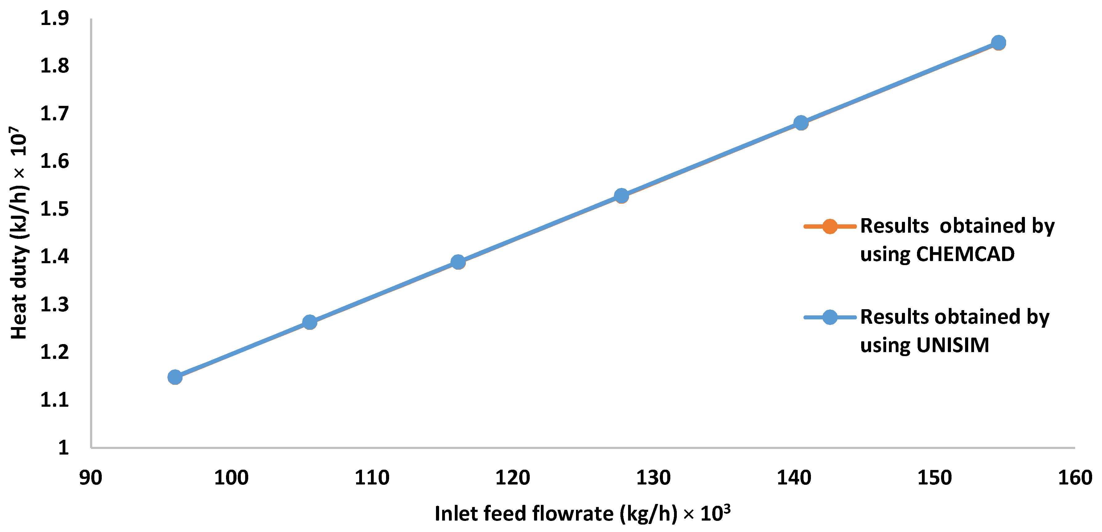
3.3. Effect of Increasing the Inlet HP Separator Feed Flow Rate on the Gas Flow Rate, Methane Mole Fraction, and Heat Required by the Preheater

The results of the HP separator inlet feed flow rate changes on the produced gas, as well as on the methane mole fraction, while keeping other parameters such as temperature, feed composition, and pressure constant, are presented in

Table 6. Feed flow rate effect on the methane mole fraction and on the outlet gas flow (CHEMCAD).

Inlet Feed Flow Rate × 103 (kg/h)	Outlet Gas Flow Rate × 104 (kmol/h)	Mole Fraction of Methane in the Outlet Gas Stream
95.97	1.9100	0.7560
105.57	2.1009	0.7560
116.12	2.3110	0.7560
127.74	2.5421	0.7560
140.51	2.7964	0.7560
154.56	3.0759	0.7560

and

Table 7. Effect of changing inlet feed flow rate on the produced methane mole fraction and on the outlet gas flow rate (UniSim).

Inlet Feed Flow Rate × 103 (kg/h)	Outlet Gas Flow Rate × 104 (kmol/h)	Mole Fraction of Methane in the Outlet Gas Stream
95.97	1.9660	0.7412
105.57	2.0934	0.7412
116.12	2.2302	0.7412
127.74	2.3806	0.7412
140.51	2.5517	0.7412
154.56	2.7562	0.7412

. These values were obtained using the two simulation software packages. The simulation results show that successive incremental increases of 10% in the inlet flow significantly increased the created gas flow rate from 1.91 × 10⁴ to 3.08 × 10⁴ kg/h (CHEMCAD) and from 1.9661 × 10⁴ to 2.7562 × 10⁴ kg/h (UniSim), which explains the available capacity of the HP separator to accommodate an increased inlet flow rate. Moreover, the methane mole fraction remained constant at 0.756045 and 0.741194 in CHEMCAD and UniSim, respectively, since the outlet gas composition is not a function of the inlet flow rate. The composition of the feed, as well as pressure and temperature, are the parameters that influenced the separation process equilibrium constant.

Similar to the rate of flow of the vapour, the preheater heating duty exhibits a direct relationship with the inlet feed rate. Hence, the heating duty increased from 11.47 to 18.48 GJ/h in both simulation software packages, when the feed flow was changed from 95.97 × 10³ to 154.56 × 10³ kg/h, as shown in Figure 5. A remarkable increase in the heating duty of the liquid hydrocarbons can be seen when the inlet feed flow rate of the HP separator was increased, since it required more energy to keep the process temperature constant.

3.4. Phase Envelope

The phase envelope of the gas stream was generated by using the simulation software packages, as shown in Figure 6. The figure illustrates that the operating condition (P = 80 bar, T = 43 °C) lies very close to the dew line of the phase envelope. Thus, any movement along a straight line to the left or right (by changing the temperature) results in a change of the phase; i.e. it results in a change in the rate of the gas production. A similar effect can be noticed by increasing or decreasing the pressure. Consequently, the HP separator temperature increases, and its pressure reduces (i.e., to 58 °C and 2360 kPa, respectively); thus, the pressure change effect on the state of the produced gas does not occur since the gas will be at the cricondentherm point, the phase envelope maximum temperature, as illustrated in Figure 6. Moreover, it will increase the HP separator gas productivity and reduce the cost of heating in the preheater, as discussed in Section 3.1 and Section 3.2.

4. Conclusions and Further Work

Overall, this study highlights the ability of using commercial simulation software packages, such as CHEMCAD, to simulate industrial processes. Furthermore, it shows that the PR model thermodynamics package gives the best fit in the simulation of hydrocarbon processes, since the obtained results were comparable to the measured values from real industrial data. Thus, it confirms the validity of the model, which is required before completing any further study (e.g., sensitivity study or optimization). This validates the approach used in the selection of the thermodynamics method for the simulation of the industrial processes.

From the results of the sensitivity study, it can be concluded that changing the pressure influences gas production significantly. Accordingly, it is advisable to operate the HP separator at lower pressure. However, the selection of the operating pressure must meet other process unit operation requirements. Moreover, increasing the temperature or the inlet feed flow rate may have a similar effect, since the rate of gas production is increased. Nevertheless, it is necessary to evaluate this change because it affects the preheater heating duty (e.g., it is directly proportional to the inlet flow rate while it has an inverse relationship with the temperature of the feed stream). The selected operating condition (P = 80 bar, T = 43 °C) is critical, since it lies on the dew point line of the phase envelope. As a consequence, it is expected that the gas may enter the two-phase region, if the temperature or the pressure decreases. Further investigation is recommended to optimize process-operating conditions, in order to fully utilize the capacity of the HP separator. Moreover, energy analyses can be conducted to utilize and recover any otherwise wasted heat.

References

1. Manning, F.S.; Thompson, R.E. Oilfield Processing of Petroleum: Crude Oil; Pennwell Books: Tulsa, OK, USA, 1991; Volume 2. [Google Scholar]
2. Mokhatab, S.; Poe, W.A. Handbook of Natural Gas Transmission and Processing; Gulf Professional Publishing: Cambridge, MA, USA, 2012. [Google Scholar]
3. Abdel-Aal, H.K.; Aggour, M.A.; Fahim, M.A. Petroleum and Gas Field Processing; CRC Press: Boca Raton, FL, USA, 2003. [Google Scholar]
4. Lieberman, N.P.; Lieberman, E.T. Working Guide to Process Equipment; McGraw-Hill Professional: New York, NY, USA, 2008. [Google Scholar]
5. Seader, J.D.; Henley, E.J.; Roper, D.K. Separation Process Principles; John Wiley & Sons, Inc.: Hoboken, NJ, USA, 1998. [Google Scholar]
6. Devold, H. Oil and Gas Production Handbook: An Introduction to Oil and Gas Production; Lulu. com: Morrisville, NC, USA, 2013. [Google Scholar]
7. Gudmestad, O.T.; Zolotukhin, A.B.; Jarlsby, E.T. Petroleum Resources with Emphasis on Offshore Fields; WIT Press: Billerica, MA, USA, 2010. [Google Scholar]
8. Peng, D.-Y.; Robinson, D.B. A new two-constant equation of state. Ind. Eng. Chem. Fundam. 1976, 15, 59–64. [Google Scholar] [CrossRef]
9. Soave, G. Equilibrium constants from a modified Redlich-Kwong equation of state. Chem. Eng. Sci. 1972, 27, 1197–1203. [Google Scholar] [CrossRef]
10. Gmehling, J.; Kolbe, B.; Kleiber, M.; Rarey, J. Chemical Thermodynamics for Process Simulation. Wiley-VCH Verlag &, Co. KGaA: Weinheim, Germany, 2012. [Google Scholar]
11. Wei, Y.S.; Sadus, R.J. Equations of state for the calculation of fluid-phase equilibria. AlChE J. 2000, 46, 169–196. [Google Scholar] [CrossRef]
12. Gutierrez, J.P.; Benítez, L.A.; Martínez, J.; Ale Ruiz, L.; Erdmann, E. Thermodynamic Properties for the Simulation of Crude Oil Primary Refining. Int. J. Eng. Res. Appl. 2014, 4, 190–194. [Google Scholar]
13. Sengers, J.V.; Kayser, R.; Peters, C.; White, H. Equations of State for Fluids and Fluid Mixtures; Elsevier: Amsterdam, The Netherlands, 2000; Volume 5. [Google Scholar]
14. Valderrama, J.O. The state of the cubic equations of state. Ind. Eng. Chem. Res. 2003, 42, 1603–1618. [Google Scholar] [CrossRef]
15. De Hemptinne, J.C.; Ledanois, J.-M. Select Thermodynamic Models for Process Simulation: A Practical Guide Using a Three Steps Methodology; Editions Technip: Paris, France, 2012. [Google Scholar]
16. Chemstations. CHEMCAD Help. 2018. Available online: https://www.chemstations.eu (accessed on 1 October 2018).
17. De Hemptinne, J.; Behar, E. Thermodynamic modelling of petroleum fluids. Oil Gas Sci. Technol. Rev. IFP 2006, 61, 303–317. [Google Scholar] [CrossRef]
18. Edwards, J.E. Process Modelling Selection of Thermodynamic Methods; P & I Design Ltd.: Thornaby, UK, 2000. [Google Scholar]
19. Edwin, M.; Abdulsalam, S.; Muhammad, I.M. Research. Process Simulation and Optimization of Crude Oil Stabilization Scheme Using Aspen-HYSYS Software. Int. J. Recent Trends Eng. Res. 2017, 3. [Google Scholar] [CrossRef]
20. Towler, G.; Sinnott, R.K. Chemical Engineering Design: Principles, Practice and Economics of Plant and Process Design; Elsevier: Waltham, MA, USA, 2012. [Google Scholar]
21. Gil Chaves, I.D.; López, J.R.G.; García Zapata, J.L.; Leguizamón Robayo, A.; Rodríguez Niño, G. Process simulation in chemical engineering. In Process Analysis and Simulation in Chemical Engineering; Springer: Basel, Switzerland, 2016; pp. 1–51. [Google Scholar]
22. Michelsen, M.L. Calculation of phase envelopes and critical points for multicomponent mixtures. Fluid Phase Equilib. 1980, 4, 1–10. [Google Scholar] [CrossRef]
Figure 1. Thermodynamics model selection chart. Reproduced with permission from Towler, G. and Sinnott, R.K., Chemical engineering design: principles, practice and economics of plant and process design; published by Elsevier, 2012. [20].
Processes 06 00219 g001
Figure 2. A diagram of the separation process of crude oil developed by using the CHEMCAD Simulation Software package.
Processes 06 00219 g002
Figure 3. HP separator pressure effect on the produced methane mole fraction, the produced gas flow and on the heating duty of the preheater rate.
Processes 06 00219 g003
Figure 4. HP separator temperature effect on the heating duty of the preheater.
Processes 06 00219 g004
Figure 5. Effect of HP separator feed flow rate on the heating duty of the preheater.
Processes 06 00219 g005
Figure 6. Phase envelope created by using the CHEMCAD Simulation Software package.
Processes 06 00219 g006