Second-Order Symmetric Smoothed Particle Hydrodynamics Method for Transient Heat Conduction Problems with Initial Discontinuity

Abstract

To eliminate the numerical oscillations appearing in the first-order symmetric smoothed particle hydrodynamics (FO-SSPH) method for simulating transient heat conduction problems with discontinuous initial distribution, this paper presents a second-order symmetric smoothed particle hydrodynamics (SO-SSPH) method. Numerical properties of both SO-SSPH and FO-SSPH are analyzed, including truncation error, numerical accuracy, convergence rate, and stability. Experimental results show that for transient heat conduction with initial smooth distribution, both FO-SSPH and SO-SSPH can achieve second-order convergence, which is consistent with the theoretical analysis. However, for one- and two-dimensional conduction with initial discontinuity, the FO-SSPH method suffers from serious unphysical oscillations, which do not disappear over time, and hence it only achieves first-order convergence; while the present SO-SSPH method can avoid unphysical oscillations and has second-order convergence rate. Therefore, the SO-SSPH method is a feasible tool for solving transient heat conduction problems with both smooth and discontinuous distributions, and it is easy to be extended to high dimensional cases.

1. Introduction

Heat transfer is generally defined as the phenomenon where heat is spread from one system or one part to another, and can be divided into three modes: heat conduction, heat convection, and thermal radiation. As the main form of heat transfer in solids, heat conduction is applied in many industrial fields, such as rubber vulcanization, steel forgings heating, and the design of thermal conductors and insulation equipment. It is of high importance for industrial production to explore the inherent law of heat conduction and to analyze the temperature distribution in heat conduction processes.

Theoretical methods cannot, in general, solve these complex heat transfer problems, while physical experiments suffer from high measurement cost. Based on computational simulations the Numerical Heat Transfer (NHT) technology [1] has been rapidly developed and the related theories have made great progress. Numerical methods for solving heat transfer problems are mainly mesh-based methods, such as finite difference methods (FDM) [2], finite volume methods (FVM), and finite element methods (FEM) [3]. In recent years, due to the inherent advantages, meshless methods have received much attention and experienced rapid development. The major difference between mesh-based methods and meshless ones is that, in meshless methods, only node information is needed and the predefined node connectivity is not necessary. Zhang et al. [4] applied the Lattice Boltzmann method (LBM) to solve the nonlinear heat conduction equation. Singh et al. [5] used the Element-Free Galerkin (EFG) method to simulate transient heat conduction problems in isotropic homogeneous objects. As one of the earliest and most powerful meshless methods, the smoothed particle hydrodynamics (SPH) [6,7] method invented for astrophysical problems has been extended to complex fluid dynamics problems, especially for those with free surface and moving interfaces. Excellent reviews of the development of SPH and its diverse applications have been provided [6,8,9,10,11,12,13,14]. The development of SPH for heat conduction problems was mainly completed after the 2000s; we review the relative works below. It is worth noting that the SPH formulations for heat equations are by no means complete, and we will focus on the most representative and promising ones. Although great success and diverse applications have been achieved, there exist two inherent drawbacks [6] in the traditional SPH method: first, the boundary deficiency due to truncated kernel support of particles close to the boundary and second, accuracy degeneration when the particle distribution becomes highly irregular. The accuracy degeneration problem is closely related to the lack of completeness of the SPH approximations [15]. To remedy these two drawbacks, several corrective techniques have been proposed, generating many corrective methods such as the corrective smoothed particle method (CSPM) [16], modified smoothed particle hydrodynamics (MSPH) [17] method, and moving least squares particle hydrodynamics (MLSPH) [18] method.

As conduction is often involved in other processes (e.g., viscous flow), there have been only a few attempts to entirely and exclusively solve the conduction problems using traditional SPH. For the discretization of the heat equation, there are three different ways. A simple discretization of the heat equation in SPH is obtained by firstly estimating the heat flux using the standard first derivative approximation, and then estimating the divergence in a second step. This method was originally used by Lucy [19] to simulate the thermal energy evaluation in the modeling of collapse and fission of optical thick protostar. The numerical results indicated that the log of density agreed to within approximately 1% of the exact solution. However, the disagreement between the exact solution and the SPH estimate of the divergence of the flux increased by 25% for particles close to the surface boundary. To remedy the boundary deficiency problem, Jeong et al. [20] deduced consistent estimation of near-boundary corrections for system variables using the ghost particle method and successfully verified this strategy against heat conduction tests. However, as shown by Brookshaw [21], this method was sensitive to distorted particle distribution, which can be traced to double differentiation of the kernel. Furthermore, another practical disadvantage is that, with an intermediate variable, the heat flux needs to be computed and stored in a separate SPH loop. The second method is the standard SPH kernel approximation of the second derivatives pioneered by Takeda et al. [22], which is sensitive to particle disorder [20] and may lead to divergence of the simulation. To remedy the divergence caused by distorted particle distributions, Chaniotis et al. [23] developed a periodic re-initialization (remeshing) technique. They found that the SPH methodology with remeshing procedure is capable of direct numerical simulation (DNS) quality simulations. In the above two methods, either a double calculation of the first derivative or a calculation of the second derivative of the kernel is needed. Both are sensitive to particle disorder that will most likely occur in fluid flows. It is hence advantageous to use a simpler SPH approximation of the Laplacian operator, which should only involve first-order derivatives of the kernel. This idea is commonly used now for heat conduction in SPH [10,11,12,14,24,25,26,27,28,29]. Such a method was pioneered by Brookshaw [21], further developed by Cleary [24,25], and its three-dimensional derivation was given by Jubelgas et al. [26] and Rook et al. [27]. To take into account a discontinuous thermal conductively with continuous heat flux across the material interfaces, Cleary and Monaghan [25] proposed to replace the averaged conductivity by its harmonic mean, such that multiple materials with substantially different conductivities and specific heat can be accurately simulated [28,29]. Based on Taylor series expansion both for regular and irregular particle distributions, Fatehi and Manzari [30] analyzed the truncation errors in the above three SPH approximations for second derivative and found that none of the three schemes has first-order completeness. A new scheme for second derivatives was proposed using a modified renormalization tensor and applied to heat conduction problem. The key idea is similar as that in the MSPH method [17], where kernel derivatives are involved in the modifications. Recently, Francomano and Paliaga [31] highlighted the numerical insights in MSPH approximations and found that the request for greater accuracy needs kernel function derivatives with order up to the desired accuracy order in approximating the function or higher for the derivatives.

For heat conduction problems, there are few related studies using the corrective SPH methods. Early explorations are due to Chen et al. [16] and Zhang and Betra [17]. Recently, Jiang et al. [32] presented the first-order symmetric smoothed particle hydrodynamics (FO-SSPH) method (named because the Taylor series of the function is expanded up to first derivatives), which has second-order accuracy and the symmetry property of the moment matrix. Furthermore, it does not involve kernel derivatives and can be directly applied to mixed boundary conditions. Although the FO-SSPH method can more effectively improve the numerical accuracy and stability than the standard SPH [32], it can only approximate the first-order spatial derivatives directly. Therefore, heat flux terms have to be introduced to transform the second-order heat equation into two first-order partial differential equations. Similar to the Forward Time Central Space (FTCS) method [33], FO-SSPH is only applicable for heat conduction problems with smooth temperature distribution. If the initial distribution has a discontinuity, unphysical oscillations will be inevitable and they cannot damp out naturally. This is because the temperature gradient at a discontinuous position tends to be infinite in theory, while the approximated first derivative in Taylor expansion can only be a finite value, so the introducing of the heat fluxes will magnify the error at this time. Therefore, it is difficult for FO-SSPH to solve transient heat conduction problems with initial discontinuity. Jiang et al. [32] concluded that the FO-SSPH has second-order convergence rate through numerical experiments. However, through theoretical analysis and numerical tests, we found that it is true for transient heat conduction problems with initial smooth distribution, but the FO-SSPH has only first-order convergence rate for problems with initial discontinuity.

Based on the above discussion, a second-order symmetric smoothed particle hydrodynamics (SO-SSPH) method (named because the Taylor series of the function is expanded up to second derivatives) is proposed to approximate second-order spatial derivatives directly in this paper to eliminate the unphysical oscillations. In this method, the second-order Taylor series is used, and symmetric moment matrices are obtained. It can directly approximate second-order derivatives. Numerical characteristics including truncation error, numerical accuracy, convergence rate, and stability of both FO-SSPH and SO-SSPH are analyzed theoretically and numerically. One key superiority of SO-SSPH to the MSPH method [17] and the scheme of Fatehi and Manzari [30] is that no kernel derivatives are needed in the calculation and the moment matrix is symmetric. This offers many numerical advantages including more choices for the kernel and saving computing resources. Numerical results show that, for transient heat conduction with initial smooth distribution, both FO-SSPH and SO-SSPH can achieve second-order convergence, which is consistent with the theoretical analysis. However, for both one- and two-dimensional transient heat conduction problems with a discontinuous initial distribution, the FO-SSPH method has only first-order convergence rate due to numerical oscillations, while the SO-SSPH method avoids unphysical oscillations and achieves second-order convergence.

2. Transient Heat Conduction Problem

In the Cartesian coordinate system, the governing equation for two-dimensional transient heat conduction problems reads

$$\rho c_p\frac{\partial T}{\partial t}=k_x\frac{{\partial }^{2}T}{\partial x^2}+k_y\frac{{\partial }^{2}T}{\partial y^2}+G,\mathrm{in}\mathsf{\Omega }$$

(1)

where $T$ is temperature, $\rho$ is material density, $c_p$ is material specific heat capacity, $G$ is source term, $\mathsf{\Omega }$ is the computational domain, $k_x$ and $k_y$ are thermal conductivity coefficients in $x$ and $y$ directions, respectively. These coefficients are influenced by many factors, such as temperature and material. For simplicity, we assume herein that both of them are constants, meaning that the transient heat conduction equation is linear.

To close Equation (1), the initial condition is

$$T(x,y,0)=T_0(x,y),\mathrm{in}\mathsf{\Omega }$$

(2)

and Dirichlet boundary condition follows

$$T(t)=T_1,\mathrm{on}{\mathsf{\Gamma }}_{\mathrm{D}}$$

(3)

and Neumann boundary condition is

$$q·n-bT=0,\mathrm{on}{\mathsf{\Gamma }}_{\mathrm{N}}$$

(4)

where $T_0$ is initial temperature distribution, $T_1$ is boundary temperature, $bT$ is heat source on the boundary, $q=(q_x,q_y)=(-k_x\frac{\partial T}{\partial x},-k_y\frac{\partial T}{\partial y})$ represents heat flux, $n={(n_x,n_y)}^T$ is the unit normal vector on the boundary, ${\mathsf{\Gamma }}_{\mathrm{D}}\cup {\mathsf{\Gamma }}_{\mathrm{N}}=\partial \mathsf{\Omega }$ is the boundary of the domain, and ${\mathsf{\Gamma }}_{\mathrm{D}}\cap {\mathsf{\Gamma }}_{\mathrm{N}}=\varnothing$.

If we further assume that there is no heat source, then Equation (1) reduces to

$$\frac{\partial T}{\partial t}={\kappa }_x\frac{{\partial }^{2}T}{\partial x^2}+{\kappa }_y\frac{{\partial }^{2}T}{\partial y^2}$$

(5)

where ${\kappa }_x=k_x/\rho c_p$ and ${\kappa }_y=k_y/\rho c_p$. Introducing the heat fluxes as intermediate variables, the second-order heat conduction Equation (5) can be transformed into the following first-order system as

$$\{\begin{array}{l}{q}_x=-{\kappa }_x\frac{\partial T}{\partial x}\\ q_y=-{\kappa }_y\frac{\partial T}{\partial y}\\ \frac{\partial T}{\partial t}=-\nabla ·q\end{array}$$

(6)

3. SO-SSPH Method

3.1. SPH Method

In SPH, the domain $\mathsf{\Omega }$ is represented by a finite number of particles, each of which has density, mass, temperature, and other relevant physical quantities. Kernel approximation and particle approximation are the two key ideas in standard SPH method [6,7].

For any physical quantity $f$ at position ${\mathit{x}}_i=(x_i,y_i)$, the SPH kernel approximation of its gradient can be expressed as [7]

$$\langle \nabla f_i\rangle ={\displaystyle {\int }_{\mathsf{\Omega }}f(\mathit{x})}\nabla Wd\mathit{x}-f_i{\displaystyle {\int }_{\mathsf{\Omega }}\nabla Wd\mathit{x}}$$

(7)

where $f_i=f({\mathit{x}}_i)$, $\langle ·\rangle$ represents the approximation operator, $W=W({\mathit{x}}_i-\mathit{x},h)$ is the kernel function, $\nabla W$ is the kernel gradient, and $h$ is the smoothing length. The kernel is required to own properties of normalization, symmetry, compactness, and convergence to Dirac function [7]. The cubic spline function is usually employed as the kernel.

Applying particle approximation to the integral terms in Equation (7), we obtain

$$\langle \nabla f_i\rangle ={\displaystyle \sum _j(f_j-f_i)}{\nabla }_i{W}_{ji}\Delta V_j$$

(8)

where ${\nabla }_i{W}_{ji}=\frac{\partial W(\left|{\mathit{x}}_j-{\mathit{x}}_i\right|,h)}{\partial {\mathit{x}}_i}$ and $\Delta V_j$ is the volume of $j$th particle.

3.2. SO-SSPH Method

The Taylor series for a function $f(x,y)$ around point $\left(x_i,y_i\right)$ in a two-dimensional domain gives

$$\begin{array}{cc}\hfill f(x,y)=& f_i+(x-x_i)f_{i,x}+(y-y_i)f_{i,y}+\frac{1}{2}{(x-x_i)}^2{f}_{i,xx}\hfill \\ & +\frac{1}{2}{(y-y_i)}^2{f}_{i,yy}+(x-x_i)(y-y_i)f_{i,xy}+\mathrm{O}(|\mathit{x}-{\mathit{x}}_i{|}^3)\hfill \end{array}$$

(9)

where $f_{i,x}:=\frac{\partial f}{\partial x}{|}_{\mathit{x}={\mathit{x}}_i},f_{i,y}:=\frac{\partial f}{\partial y}{|}_{\mathit{x}={\mathit{x}}_i},f_{i,xx}:=\frac{{\partial }^{2}f}{\partial x^2}{|}_{\mathit{x}={\mathit{x}}_i},$ $f_{i,yy}:=\frac{{\partial }^{2}f}{\partial y^2}{|}_{\mathit{x}={\mathit{x}}_i},f_{i,xy}:=\frac{{\partial }^{2}f}{\partial x\partial y}{|}_{\mathit{x}={\mathit{x}}_i}$.

We neglect the third- and higher-order derivatives and multiply both sides with a compactly supported function $W_k:=W_k(\left|\mathit{x}-{\mathit{x}}_i\right|,h),(k=1,2,\cdots 5)$. Then, integrating over the computational domain and approximating the integrals with Riemman sum, we can get a system with five unknowns in matrix form as

$$M_{5\times 5}{u}_{5\times 1}=b_{5\times 1}$$

(10)

where $M_{5\times 5}=(M_{kl}),$ $b_{5\times 1}=(b_k),$ $u_{5\times 1}={(\langle f_{i,x}\rangle ,\langle f_{i,y}\rangle ,\langle f_{i,xx}\rangle ,\langle f_{i,yy}\rangle ,\langle f_{i,xy}\rangle )}^T,$ $M_{kl}={\displaystyle \sum _j{P}_l{W}_k\Delta V_j},$ $b_k={\displaystyle \sum _j(f_j-f_i)W_k\Delta V_j}$, $k,l=1,2\cdots ,5$.

Assume that $W_k=P_k{W}_{ji}$ and $P_1=x_{ji},P_2=y_{ji}$, $P_3=\frac{1}{2}{x_{ji}}^2$, $P_4=\frac{1}{2}{y_{ji}}^2,P_5=x_{ji}{y}_{ji}$, where $x_{ji}=x_j-x_i$, $y_{ji}=y_j-y_i$. Then the second derivatives are approximated as

$$\langle f_{i,xx}\rangle =\left\{0,0,1,0,0\right\}{M}_{5\times 5}^{-1}{b}_{5\times 1}\mathrm{and}\langle f_{i,yy}\rangle =\left\{0,0,0,1,0\right\}{M}_{5\times 5}^{-1}{b}_{5\times 1}$$

(11)

As the function is expanded up to second derivatives, and the moment matrix $M_{5\times 5}$ is symmetric, it is referred to as second-order symmetric smoothed particle hydrodynamics (SO-SSPH) method.

When the function is expanded up to first derivatives, the resulting system becomes

$$M_{2\times 2}{u}_{2\times 1}=b_{2\times 1}$$

(12)

where $M_{2\times 2}=(M_{kl}),b_{2\times 1}=(b_k),u_{2\times 1}={(\langle f_{i,x}\rangle ,\langle f_{i,y}\rangle )}^T,M_{kl}={\displaystyle \sum _j{P}_l{W}_k\Delta V_j,}{b}_k={\displaystyle \sum _j(f_j-f_i)W_k\Delta V_j}$, $k,l=1,2$.

The first derivatives are approximated as

$$\langle f_{i,x}\rangle =\left\{1,0\right\}{M}_{2\times 2}^{-1}{b}_{2\times 1}\mathrm{and}\langle f_{i,y}\rangle =\left\{0,1\right\}{M}_{2\times 2}^{-1}{b}_{2\times 1}$$

(13)

This was referred to as the first-order symmetric smoothed particle hydrodynamics (FO-SSPH) method by Jiang et al. [32].

To effectively solve heat conduction problems with discontinuous initial distributions, different strategies for spatial derivative approximations are investigated in this paper. Approximating the second-order spatial derivatives in Equation (5) using the SO-SSPH method, and approximating the heat flux terms and their derivatives in Equation (6) using the FO-SSPH method were carried out. In theory, time integration can be completed by any effective algorithms, and for convenience, we use the Euler forward difference scheme herein.

4. Numerical Analysis

4.1. Truncation Error

To approximate the spatial derivatives, both FO-SSPH and SO-SSPH methods reserve the first several terms and neglect the rest in Taylor series expansion. Obviously, this introduces deviation, which is called truncation error [34,35] and denoted by $TE$.

In the SO-SSPH method, the exact matrix form for the derivative approximations gives

$$M_{5\times 5}{u}_{5\times 1}={\tilde{b}}_{5\times 1}$$

(14)

where ${\tilde{b}}_{5\times 1}=({\tilde{b}}_k),{\tilde{b}}_k={\displaystyle \sum _j(f_j-f_i)W_k\Delta V_j+{\displaystyle \sum _j\mathrm{O}(|{\mathrm{x}}_j-{\mathrm{x}}_i{|}^3)}{W}_k\Delta V_j},k=1,2\cdots ,5$. Therefore, the truncation error corresponding to the approximation of second-order spatial derivatives in SO-SSPH method writes

$$\begin{array}{cc}\hfill TE& ={\beta }_x(f_{i,xx}-\langle f_{i,xx}\rangle )+{\beta }_y(f_{i,yy}-\langle f_{i,yy}\rangle )\hfill \\ & ={\beta }_x\{0,0,1,0,0\}{M}_{5\times 5}^{-1}(b_{5\times 1}-{\tilde{b}}_{5\times 1})+{\beta }_y\{0,0,0,1,0\}{M}_{5\times 5}^{-1}(b_{5\times 1}-{\tilde{b}}_{5\times 1})\hfill \end{array}$$

(15)

where ${\beta }_x$ and ${\beta }_y$ are the coefficients of $\frac{{\partial }^{2}f}{\partial x^2}$ and $\frac{{\partial }^{2}f}{\partial y^2}$, respectively.

In the FO-SSPH method, the exact matrix form for the derivatives gives

$$M_{2\times 2}{u}_{2\times 1}={\tilde{b}}_{2\times 1}$$

(16)

where ${\tilde{b}}_{2\times 1}=({\tilde{b}}_k),{\tilde{b}}_k={\displaystyle \sum _j(f_j-f_i)W_k\Delta V_j+{\displaystyle \sum _j\mathrm{O}(|{\mathrm{x}}_j-{\mathrm{x}}_i{|}^2)}{W}_k\Delta V_j},k=1,2$. Therefore, the truncation error corresponding to the approximation of first-order derivatives writes

$$\begin{array}{cc}\hfill TE& ={\alpha }_x(f_{i,x}-\langle f_{i,x}\rangle )+{\alpha }_y(f_{i,y}-\langle f_{i,y}\rangle )\hfill \\ & ={\alpha }_x\{1,0\}{M}_{2\times 2}^{-1}(b_{2\times 1}-{\tilde{b}}_{2\times 1})+{\alpha }_y\{0,1\}{M}_{2\times 2}^{-1}(b_{2\times 1}-{\tilde{b}}_{2\times 1})\hfill \end{array}$$

(17)

where ${\alpha }_x$ and ${\alpha }_y$ are the coefficients of $\frac{\partial f}{\partial x}$ and $\frac{\partial f}{\partial y}$, respectively.

4.2. Numerical Accuracy

According to the definition of matrix $M_{5\times 5}$ in Equation (10), every matrix element can be represented as ${\displaystyle \sum _j{x}_{ji}^{\alpha }{y}_{ji}^{\beta }{W}_{ji}\Delta V_j},(\alpha ,\beta \in N^{+})$. Considering the symmetry property of the kernel function, the following conclusion can be drawn for evenly distributed particles as applied in this work.

$${\displaystyle \sum _j{x}_{ji}^{\alpha }{y}_{ji}^{\beta }{W}_{ji}\Delta V_j}\{\begin{array}{l}\ne 0,\mathrm{if}\alpha \mathrm{and}\beta \mathrm{are}\mathrm{even}\mathrm{numbers}\\ =0,\mathrm{otherwise}\end{array}$$

(18)

As the magnitudes of particle distances are the same, we obtain

$${\displaystyle \sum _j{x}_{ji}^{\alpha }{y}_{ji}^{\beta }{W}_{ji}\Delta V_j}=\mathrm{O}(|h{|}^{\alpha +\beta }),(\alpha \mathrm{and}\beta \mathrm{are}\mathrm{even}\mathrm{numbers})$$

(19)

where $h={(\Delta x,\Delta y)}^T$. Therefore, the moment matrix satisfies

$$M_{5\times 5}=\left(\begin{array}{ccccc}\mathrm{O}(|h{|}^2)& & & & \\ & \mathrm{O}(|h{|}^2)& & & \\ & & \mathrm{O}(|h{|}^4)& \mathrm{O}(|h{|}^4)& \\ & & \mathrm{O}(|h{|}^4)& \mathrm{O}(|h{|}^4)& \\ & & & & \mathrm{O}(|h{|}^4)\end{array}\right)$$

(20)

It can be seen that $M_{5\times 5}$ belongs to a partitioned diagonal matrix, so its inverse matrix follows as

$$M_{5\times 5}^{-1}=\left(\begin{array}{ccccc}\mathrm{O}(|h{|}^{-2})& & & & \\ & \mathrm{O}(|h{|}^{-2})& & & \\ & & \mathrm{O}(|h{|}^{-4})& \mathrm{O}(|h{|}^{-4})& \\ & & \mathrm{O}(|h{|}^{-4})& \mathrm{O}(|h{|}^{-4})& \\ & & & & \mathrm{O}(|h{|}^{-4})\end{array}\right)$$

(21)

Similarly,

$$b_{5\times 1}-{\tilde{b}}_{5\times 1}={\left(\mathrm{O}(|h{|}^4),\mathrm{O}(|h{|}^4),\mathrm{O}(|h{|}^6),\mathrm{O}(|h{|}^6),\mathrm{O}(|h{|}^6)\right)}^T$$

(22)

Therefore, Equation (15) can be expressed as

$$TE=\mathrm{O}\left(\right|h{|}^2)$$

(23)

That is to say, using the SO-SSPH method to approximate second derivatives possesses second-order accuracy.

According to the definition of matrix $M_{2\times 2}$ in Equation (12) and similar analysis, we obtain

$$M_{2\times 2}^{-1}={\left(\begin{array}{cc}\mathrm{O}(|h{|}^2)& 0\\ 0& \mathrm{O}(|h{|}^2)\end{array}\right)}^{-1}=\left(\begin{array}{cc}\mathrm{O}(|h{|}^{-2})& 0\\ 0& \mathrm{O}(|h{|}^{-2})\end{array}\right)$$

(24)

and

$$b_{2\times 1}-{\tilde{b}}_{2\times 1}=={\left(\mathrm{O}\left(\right|h{|}^4),\mathrm{O}(\left|h{|}^4\right)\right)}^{\mathrm{T}}$$

(25)

Therefore, Equation (17) can be expressed as

$$TE=\mathrm{O}\left(\right|h{|}^2)$$

(26)

That is to say, using the FO-SSPH method to approximate first derivatives possesses second-order accuracy too.

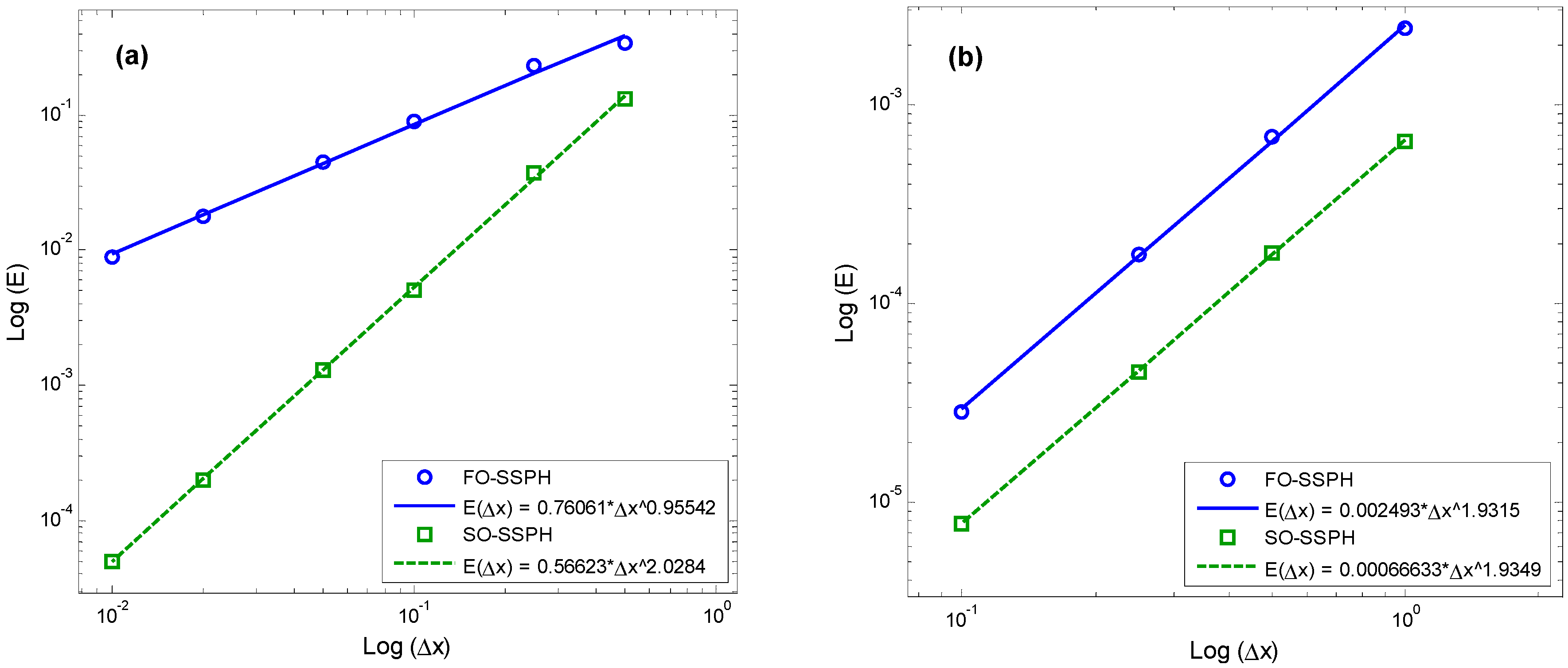
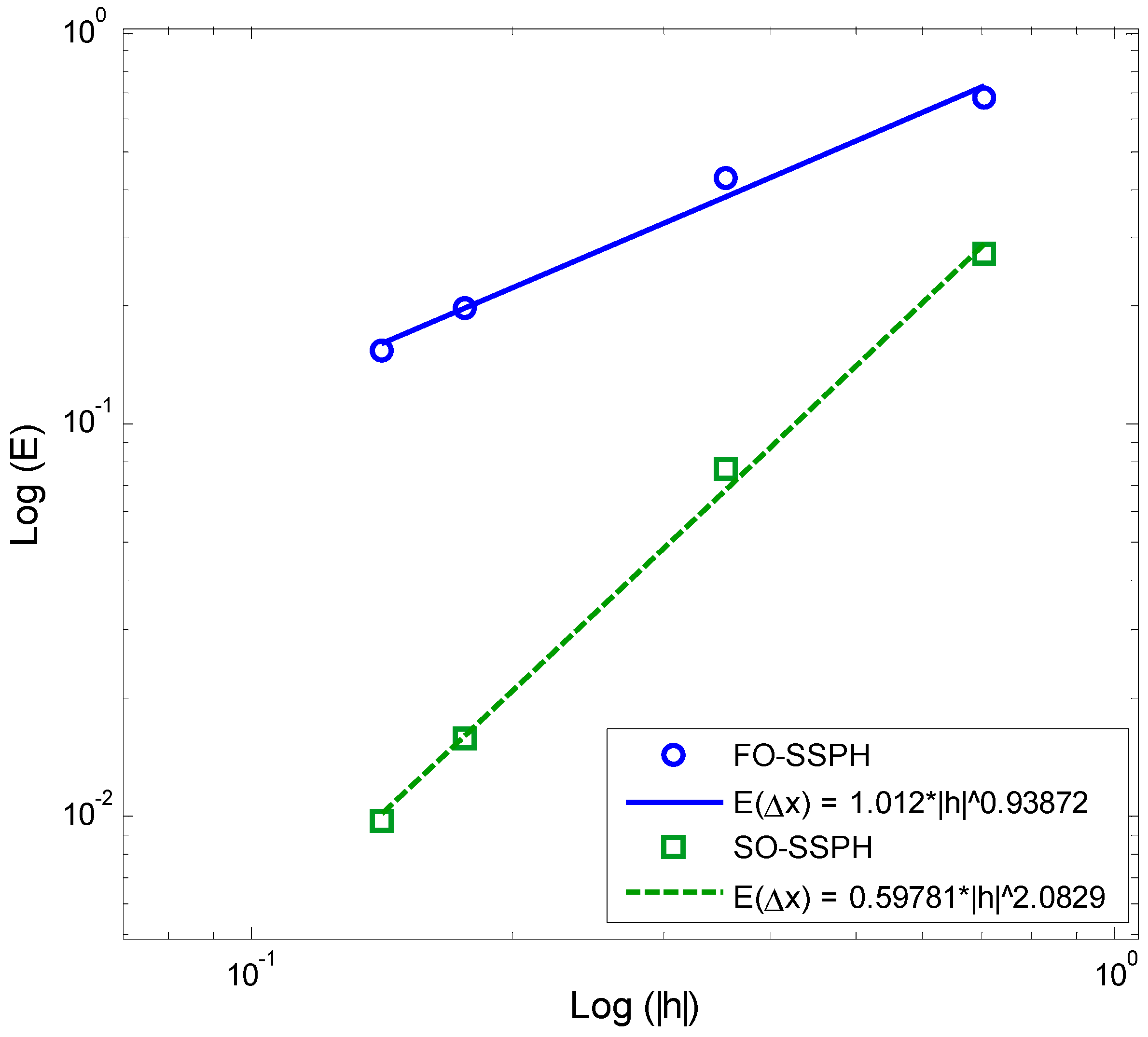
4.3. Convergence Rate

The convergence is theoretically defined to describe the degree of the closeness between numerical solution and exact solution when $\left(\Delta t,h\right)\to \left(0,0\right)$ [36]. The actual convergence rates not only depend on the discretization procedure, but also on the smoothness of the solution [37].

Assuming that the numerical error satisfies

$$\mathrm{E}=\mathrm{O}(|h{|}^q)=C|h{|}^q$$

(27)

and after taking the logarithm, we obtain

$$\log \mathrm{E}=q\log \left|h\right|+\log C$$

(28)

Therefore, the function in Equation (28) represents a straight line in log-log coordinate system, and its slope describes the convergence rate of the corresponding numerical method.

4.4. Stability Analysis

Equation (11) gives the SO-SSPH discrete form to approximate second derivatives, which can also be written as

$$\begin{array}{l}\langle f_{i,xx}\rangle ={\eta }_i{f}_i+{\displaystyle \sum _{j\ne i}{\eta }_j{f}_j}\\ \langle f_{i,yy}\rangle ={\varphi }_i{f}_i+{\displaystyle \sum _{j\ne i}{\varphi }_j{f}_j}\end{array}$$

(29)

with

$$\begin{array}{l}{\eta }_i+{\displaystyle \sum _{j\ne i}{\eta }_j}=0\\ {\varphi }_i+{\displaystyle \sum _{j\ne i}{\varphi }_j}=0\end{array}$$

(30)

Substituting Equation (29) for spatial derivatives and forward difference for time derivative into Equation (5), we obtain

$$T_i^{n+1}=T_i^n+\Delta t{\kappa }_x({\eta }_i+{{\displaystyle \sum _{j\ne i}{\eta }_{j}e}}^{\mathit{i}{\mathit{\nu }}^T{\mathit{h}}_j})T_i^n+\Delta t{\kappa }_y({\varphi }_i+{{\displaystyle \sum _{j\ne i}{\varphi }_{j}e}}^{\mathit{i}{\mathit{\nu }}^T{\mathit{h}}_j})T_i^n$$

(31)

where $\mathit{i}$ is the imaginary unit and $\mathit{\nu }$ is the column vector of the wave number in the Fourier analysis method [34,35], ${\mathit{h}}_j={({\mathit{x}}_j-{\mathit{x}}_i)}^T={(\Delta x_j,\Delta y_j)}^T$. Thus, the amplification factor is

$$\begin{array}{cc}\hfill G=& 1+\Delta t({\kappa }_x{\eta }_i+{\kappa }_y{\varphi }_i)+\Delta t{\displaystyle \sum _{j\ne i}({\kappa }_x{\eta }_j+{\kappa }_y{\varphi }_j)}\cos {\mathit{\nu }}^T{\mathit{h}}_j\hfill \\ & +\mathit{i}\Delta t{\displaystyle \sum _{j\ne i}({\kappa }_x{\eta }_j+{\kappa }_y{\varphi }_j)}\sin {\mathit{\nu }}^T{\mathit{h}}_j\hfill \end{array}$$

(32)

Taking Equation (30) into consideration, it can be simplified to

$$G=1-\Delta t{\displaystyle \sum _{j\ne i}({\kappa }_y{\eta }_j+{\kappa }_y{\varphi }_j)}(1-\cos {\mathit{\nu }}^T{\mathit{h}}_j)+\mathit{i}\Delta t{\displaystyle \sum _{j\ne i}(k_y{\eta }_j+k_y{\varphi }_j)}\sin {\mathit{\nu }}^T{\mathit{h}}_j$$

(33)

According to the von Neumann stability criterion [38], if the discrete form is stable, the amplification factor must satisfy the condition of $\left|G\right|\le 1$. For simplicity, we choose its necessary condition $\left|\mathrm{Re}(G)\right|\le 1$ in this paper, which leads to

$$0<\Delta t\le 1/\left|{\kappa }_x{\eta }_i+{\kappa }_x{\varphi }_i\right|$$

(34)

Equation (13) gives the FO-SSPH discrete form to approximate first derivatives, which also can be written as

$$\begin{array}{l}\langle f_{i,x}\rangle ={\lambda }_i{f}_i+{\displaystyle \sum _{j\ne i}{\lambda }_j{f}_j}\\ \langle f_{i,y}\rangle ={\gamma }_i{f}_i+{\displaystyle \sum _{j\ne i}{\gamma }_j{f}_j}\end{array}$$

(35)

with

$$\begin{array}{l}{\lambda }_i+{\displaystyle \sum _{j\ne i}{\lambda }_j}=0\\ {\gamma }_i+{\displaystyle \sum _{j\ne i}{\gamma }_j}=0\end{array}$$

(36)

Substituting Equation (35) for spatial derivatives and forward difference for time derivative into Equation (6), we obtain

$$\begin{array}{l}\{\begin{array}{l}{q}_{x,i}^{n+1}=-{\kappa }_x({\lambda }_i{T}_i^n+{\displaystyle \sum _j{\lambda }_j{T}_j^n})\\ q_{y,i}^{n+1}=-{\kappa }_y({\gamma }_i{T}_i^n+{\displaystyle \sum _j{\gamma }_j{T}_j^n)}\\ \frac{T_i^{n+1}-T_i^n}{\Delta t}=-({\lambda }_i{q}_{x,i}^{n+1}+{\displaystyle \sum _j{\lambda }_j{q}_{x,j}^{n+1}})-({\gamma }_i{q}_{y,i}^{n+1}+{\displaystyle \sum _j{\gamma }_j{q}_{y,j}^{n+1}})\end{array}\end{array}$$

(37)

which can be simplified to

$$T_i^{n+1}=T_i^n+\Delta t{\kappa }_x{({\lambda }_i+{\displaystyle \sum _{j\ne i}{\lambda }_j{e}^{i{\mathit{\nu }}^T{\mathit{h}}_j}})}^2{T}_i^n+\Delta t{\kappa }_y{({\gamma }_i+{\displaystyle \sum _{j\ne i}{\gamma }_j{e}^{i{\mathit{\nu }}^T{\mathit{h}}_j}})}^2{T}_i^n$$

(38)

According to the Fourier analysis, together with Equation (36), the amplification factor follows

$$G=1-{\kappa }_x\Delta t{\left[{\displaystyle \sum _{j\ne i}{\lambda }_j(1-\cos {\mathit{\nu }}^T{\mathit{h}}_j-i\sin {\mathit{\nu }}^T{\mathit{h}}_j)}\right]}^2-{\kappa }_y\Delta t{\left[{\displaystyle \sum _{j\ne i}{\gamma }_j(1-\cos {\mathit{\nu }}^T{\mathit{h}}_j-i\sin {\mathit{\nu }}^T{\mathit{h}}_j)}\right]}^2$$

(39)

and further simplification leads to

$$\begin{array}{cc}\hfill G=& 1-{\kappa }_x\Delta t\left[{\left({\displaystyle \sum _{j\ne i}{\lambda }_j(1-\cos {\mathit{\nu }}^T{\mathit{h}}_j)}\right)}^2-{\left({\displaystyle \sum _{j\ne i}{\lambda }_j\sin {\mathit{\nu }}^T{\mathit{h}}_j}\right)}^2\right]\hfill \\ & -{\kappa }_y\Delta t\left[{\left({\displaystyle \sum _{j\ne i}{\gamma }_j(1-\cos {\mathit{\nu }}^T{\mathit{h}}_j)}\right)}^2-{\left({\displaystyle \sum _{j\ne i}{\gamma }_j\sin {\mathit{\nu }}^T{\mathit{h}}_j}\right)}^2\right]\hfill \\ & +2\mathit{i}{\kappa }_x\Delta t\left({\displaystyle \sum _{j\ne i}{\lambda }_j(1-\cos {\mathit{\nu }}^T{\mathit{h}}_j)}\right)\left({\displaystyle \sum _{j\ne i}{\lambda }_j\sin {\mathit{\nu }}^T{\mathit{h}}_j}\right)\hfill \\ & +2\mathit{i}{\kappa }_y\Delta t\left({\displaystyle \sum _{j\ne i}{\gamma }_j(1-\cos {\mathit{\nu }}^T{\mathit{h}}_j)}\right)\left({\displaystyle \sum _{j\ne i}{\gamma }_j\sin {\mathit{\nu }}^T{\mathit{h}}_j}\right)\hfill \end{array}$$

(40)

According to the von Neumann stability criterion [38], if the discrete form is stable, the amplification factor must satisfy the condition of $\left|G\right|\le 1$. For simplicity, its necessary condition $\left|\mathrm{Re}(G)\right|\le 1$ is employed and we obtain

$$0<\Delta t\le \frac{1}{2\left[{\kappa }_x{\left({\displaystyle \sum _{j\ne i}\left|{\lambda }_j\right|}\right)}^2+{\kappa }_y{\left({\displaystyle \sum _{j\ne i}\left|{\gamma }_j\right|}\right)}^2\right]}$$

(41)

5. Numerical Experiments

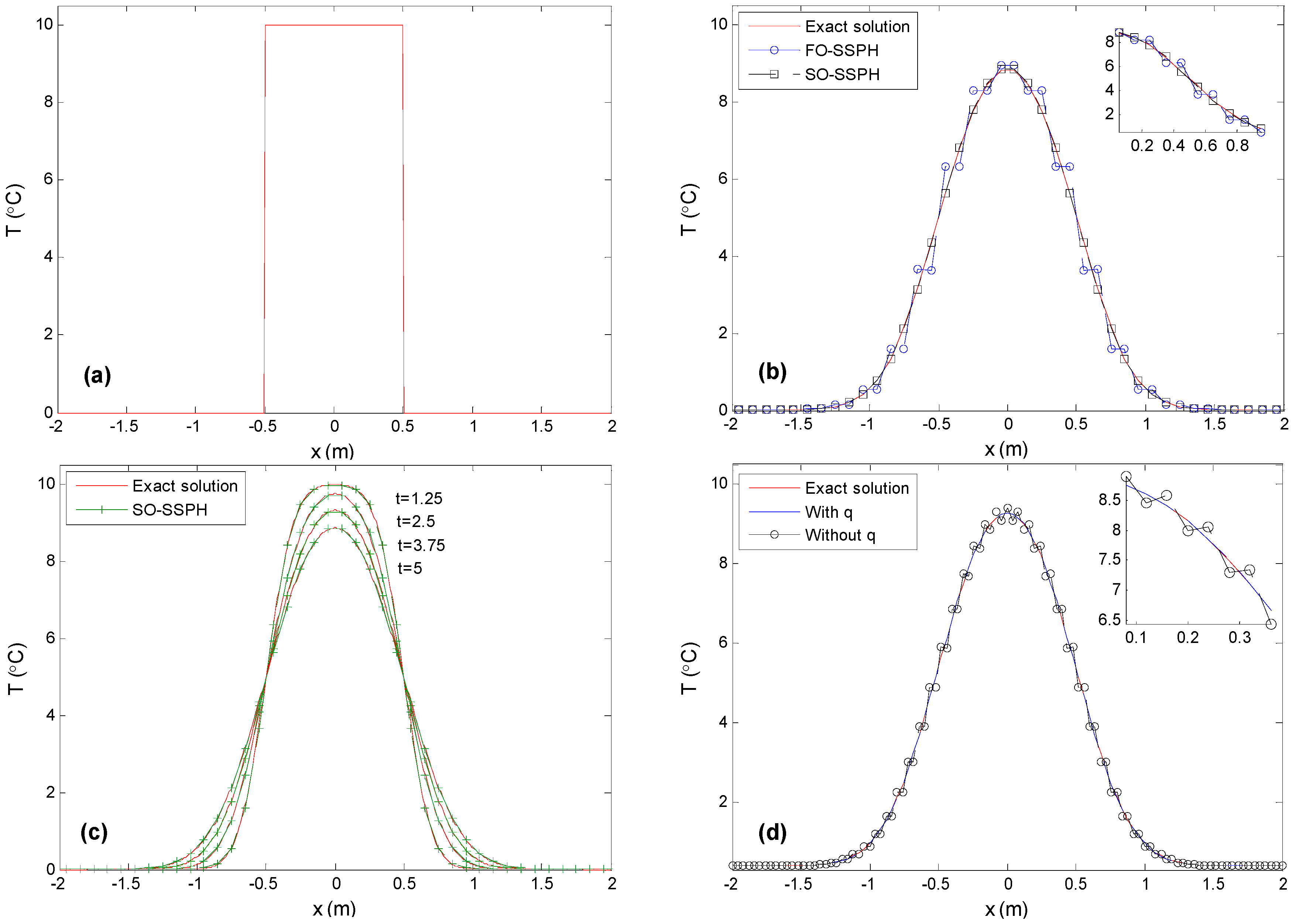
5.1. One-Dimensional Case

Considering the one-dimensional transient heat conduction problem

$$\frac{\partial T}{\partial t}={\kappa }_x\frac{{\partial }^{2}T}{\partial x^2},\mathsf{\Omega }=[-L,L]$$

(42)

with discontinuous initial condition

$$T(x,0)=\{\begin{array}{l}{T}_0,x\in [-a,a]\\ 0,\mathrm{otherwise}\end{array}$$

(43)

and boundary condition

$$T(-L,t)=0,T(L,t)=0$$

(44)

The exact solution is

$$T(x,t)=\frac{T_0}{2}\left[erf\left(\frac{a+x}{\sqrt{4t{\kappa }_x}}\right)+erf\left(\frac{a-x}{\sqrt{4t{\kappa }_y}}\right)\right]$$

(45)

in which $erf$ is the error function defined as $erf(x)=\frac{2}{\sqrt{\pi }}{\displaystyle {\int }_0^x{e}^{-{\mu }^2}}d\mu$.

The parameters of $L=2$ m, $a=0.5$ m, ${\kappa }_x=k_x/\rho c_p=0.01{\mathrm{m}}^2/\mathrm{s}$, and $T_0=10°\mathrm{C}$ are used in the simulation. The initial temperature distribution is given in Figure 1a. Both FO-SSPH and SO-SSPH use the same parameters, particle distance $\Delta x=0.1$ m, and smoothing length $h=1.05\Delta x$. According to the stability analysis given above, the stability conditions of FO-SSPH and SO-SSPH are $\Delta t\le 2\mathrm{s}$ and $\Delta t\le 0.5\mathrm{s},$ respectively. To avoid the influence of the time integration error on the subsequent spatial convergence analysis, a sufficiently small time step of $\Delta t=0.00005\mathrm{s}$ is chosen, and the simulation time is 5 s.

Numerical results of FO-SSPH and SO-SSPH are shown in Figure 1b together with the exact solution. It is seen that FO-SSPH [32] suffers from unphysical oscillations, which do not exist in the SO-SSPH solution. Temperature distributions at four different times are shown in Figure 1c where excellent agreements with exact solutions are observed as expected.

Numerical oscillations appearing in the FO-SSPH solution are mainly due to the discontinuity in the initial temperature. The temperature gradient at the discontinuous position tends to be infinity in theory, while the approximated first derivative in Taylor expansion can only be a finite value. This leads to degeneration of numerical accuracy. Therefore, for transient heat conduction problems with discontinuous initial distribution, the second-order spatial derivatives should be discretized directly to reduce error accumulation.

For further verification, the forward time central space (FTCS) method [33] is also used to solve this problem (first derivative is approximated by the central difference) and the results are shown in Figure 1d. It demonstrates that FTCS with heat fluxes suffers from unphysical oscillations too, which is consistent with the FO-SSPH results. However, without introducing the heat fluxes, FTCS (second derivative is approximated by the central difference) gives solutions without oscillations (see Figure 1d).

To further analyze the properties of the methods, we define the relative numerical error as

$$\mathrm{E}=\frac{{\displaystyle \sum \left|T^e-T^n\right|}}{{\displaystyle \sum T^e}}$$

(46)

where $T^e$ is exact temperature, $T^n$ is numerical temperature, and the summation is over all particles. Varying the values of $\Delta x$, six pairs of error data corresponding to FO-SSPH and SO-SSPH are calculated and the results are shown in

Table 1. Errors of FO-SSPH and SO-SSPH for one-dimensional heat conduction with discontinuous initial distribution.

Method	Δx (m)
	0.01	0.02	0.05	0.10	0.25	0.5
FO-SSPH	0.0089	0.0178	0.0445	0.0898	0.2297	0.3381
SO-SSPH	$5.0103\times {10}^{-5}$	$1.9993\times {10}^{-4}$	0.0013	0.0051	0.0379	0.1303

.

According to the data in Table 1, least-squares-based curve fitting is performed. Convergence rates in double logarithmic coordinates are shown in Figure 2a. It is found that FO-SSPH can only achieve first-order convergence, while SO-SSPH has second-order convergence rate. In Section 3, we have proven that both FO-SSPH for first derivative approximation and SO-SSPH for second derivative approximation possess second-order accuracy. It implies that the actual convergence rate depends not only on the accuracy of the method, but also on the smoothness of the solution. This is consistent with Kuzmin’s conclusion for mesh-based methods [37].

For further verification, and to more clearly explain the FO-SSPH defects when dealing with heat conduction problems with discontinuous initial distribution, the performances of FO-SSPH and SO-SSPH methods for solving a heat conduction problem with smooth (Gaussian) initial distribution are examined. The Gaussian initial distribution follows

$$T(x,0)=\frac{M}{\sqrt{2\pi {\sigma }_0}}\exp \left(-\frac{x^2}{2{\sigma }_0^2}\right),x\in [-15\mathrm{m},15\mathrm{m}]$$

(47)

where $M=\sqrt{2\mathsf{\pi }{\sigma }_0}$ and ${\sigma }_0=2$ m. The exact solution is written as

$$T(x,t)=\frac{{\sigma }_0}{\sqrt{{\sigma }_0^2+2{\kappa }_{x}t}}\exp \left(-\frac{x^2}{2({\sigma }_0^2+2{\kappa }_{x}t)}\right)$$

(48)

The corresponding errors are shown in

Table 2. Errors of FO-SSPH and SO-SSPH for one-dimensional heat conduction with Gaussian distribution.

Method	Δx (m)
	0.1	0.25	0.5	1.0
FO-SSPH	$2.848\times {10}^{-5}$	$1.7465\times {10}^{-4}$	$6.8262\times {10}^{-4}$	0.0024
SO-SSPH	$7.706\times {10}^{-6}$	$4.522\times {10}^{-5}$	$1.7967\times {10}^{-4}$	$6.5431\times {10}^{-4}$

, and the convergence rate curves of FO-SSPH and SO-SSPH are drawn in Figure 2b. It is seen that FO-SSPH method can achieve second-order convergence, which is in accordance with the theoretical analysis. Therefore, when the FO-SSPH method is used to deal with heat conduction problems with discontinuous initial distributions, the theoretical convergence rate cannot be achieved due to numerical oscillations.

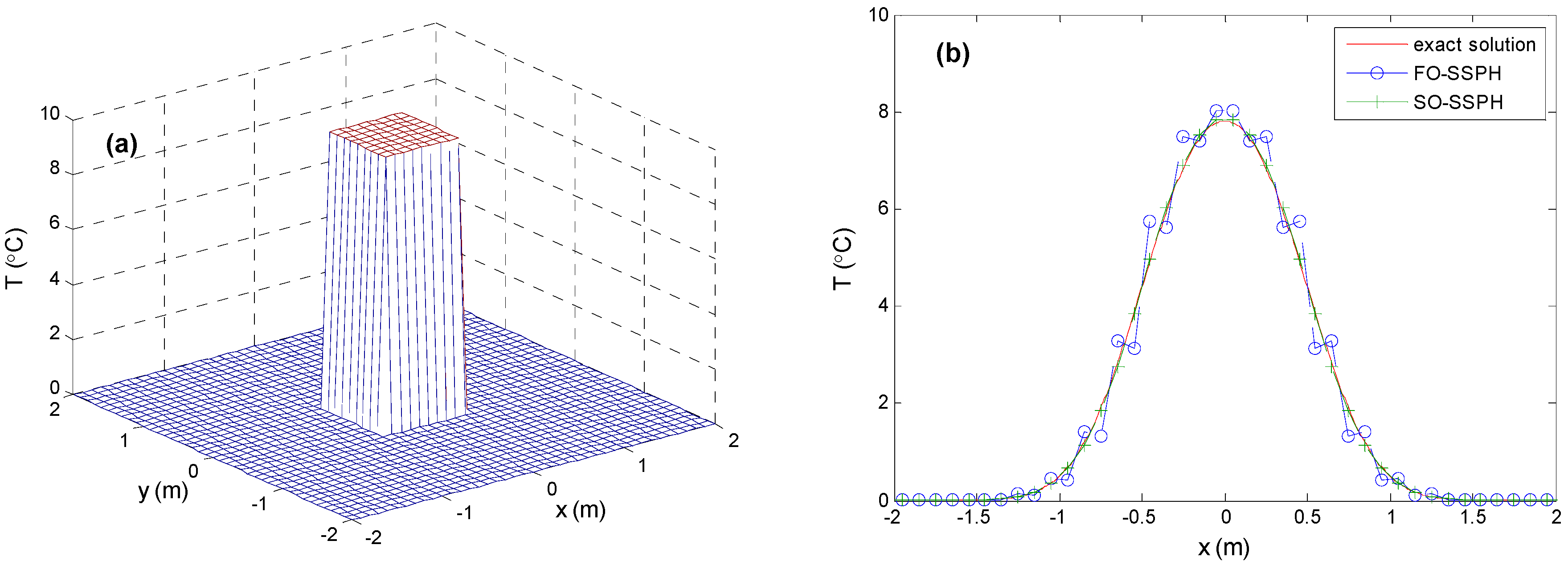
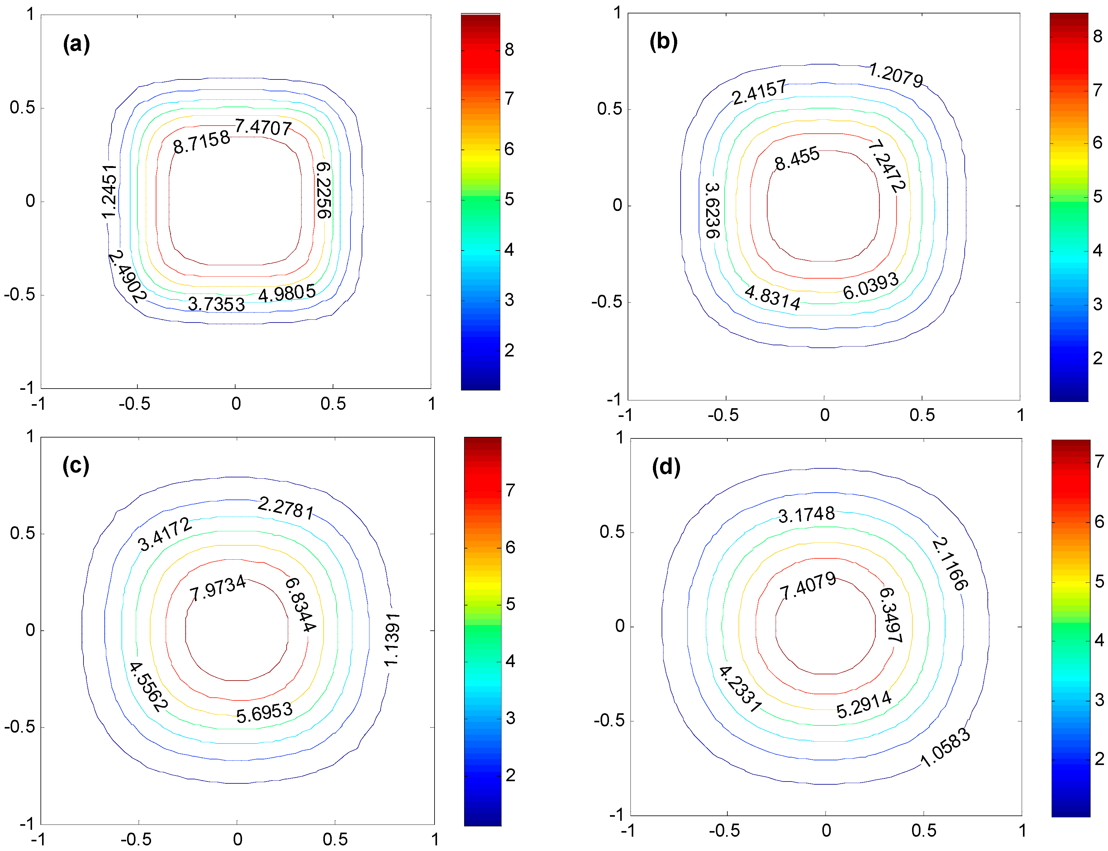
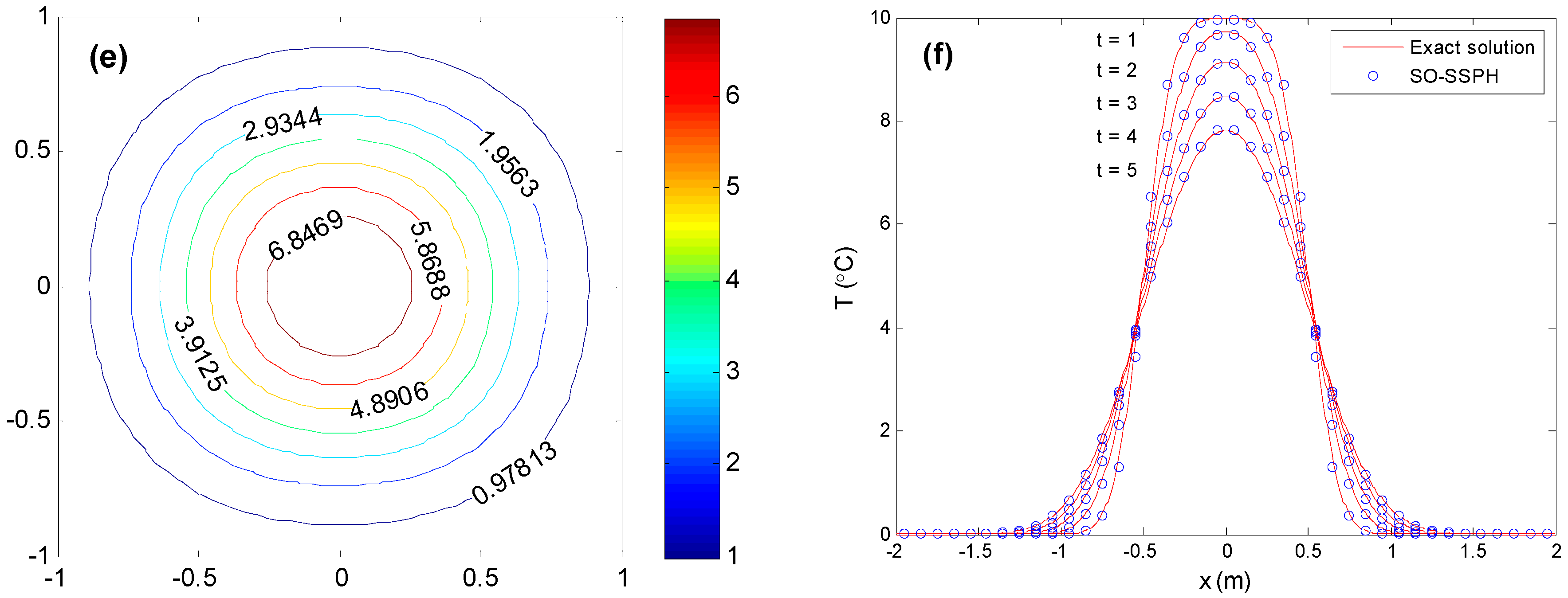
5.2. Two-Dimensional Case

Consider the two-dimensional transient heat Equation (5) with initial condition

$$T(x,y,0)=\{\begin{array}{l}{T}_0,(x,y)\in [-a,a]\times [-b,b]\\ 0,\mathrm{otherwise}\end{array}$$

(49)

and boundary condition

$$T(-L,y,t)=0,T(L,y,t)=0,T(x,-L,t)=0,T(x,L,t)=0$$

(50)

where $a<L,b<L$. The initial distribution is discontinuous and the exact solution is

$$T(x,y,t)=\frac{T_0}{4}\left[erf\left(\frac{a+x}{\sqrt{4t{\kappa }_x}}\right)+erf\left(\frac{a-x}{\sqrt{4t{\kappa }_x}}\right)\right]\left[erf\left(\frac{b+y}{\sqrt{4t{\kappa }_y}}\right)+erf\left(\frac{b-y}{\sqrt{4t{\kappa }_y}}\right)\right]$$

(51)

The parameters $L=2\mathrm{m}$, $a=b=0.5\mathrm{m}$, ${\kappa }_x={\kappa }_y=0.01$ m²/s, and $T_0=10°\mathrm{C}$ are used in the simulations. The initial temperature distribution is shown in Figure 3a. Both FO-SSPH and SO-SSPH use the same simulation parameters: particle distances $\Delta x=\Delta y=0.1\mathrm{m}$, smoothing length $h=1.1\Delta x$, time step $\Delta t=0.001\mathrm{s}$ and simulation time 5 s.

FO-SSPH and SO-SSPH are used to simulate this problem and the results at cross-section y = 0.05 m are shown in Figure 3b together with the exact solution. It is seen that for two-dimensional heat conduction with discontinuous initial distribution, the FO-SSPH method still suffers from unphysical oscillations as might be expected, but the proposed SO-SSPH does not.

To show the two-dimensional heat conduction process, temperature contours at five different times are depicted in Figure 4a–e. It is seen that with increasing time, high temperature area expands and amplitude decreases, which conforms to the law of heat conduction. In addition, each contour line is smooth, which demonstrates that there is no unphysical oscillations in the SO-SSPH solution as expected. This is more clear as shown in Figure 4f for the temperature distribution along y = 0.05 m.

Varying the values of Δx and Δy, four pairs of error data corresponding to FO-SSPH and SO-SSPH are listed in

Table 3. Errors of FO-SSPH and SO-SSPH for two-dimensional heat conduction with discontinuous initial distribution.

Method	Δx = Δy (m)
	0.10	0.125	0.25	0.5
FO-SSPH	0.1548	0.1974	0.4263	0.6867
SO-SSPH	0.0098	0.0159	0.0773	0.2719

. The convergence rate curves of FO-SSPH and SO-SSPH are shown in Figure 5. It is clear that similar to the one-dimensional case, FO-SSPH only achieves first-order convergence, whereas SO-SSPH has second-order convergence rate.

6. Discussion and Conclusions

For transient heat conduction problems with discontinuous initial distribution, a second-order symmetric smoothed particle hydrodynamics (SO-SSPH) method is proposed to approximate the second-order spatial derivative terms directly. Compared with the simulation results of the FO-SSPH method, the SO-SSPH method can effectively eliminate the unphysical oscillations in FO-SSPH. This is mainly due to the initial temperature which is discontinuous such that the local gradient tends to infinity, while the approximated first derivative can only be of a finite value. This implies that FO-SSPH is incapable of approximating the second derivatives indirectly in essence. In addition, according to the convergence analysis, it is found that for transient heat conduction problems with smooth initial distributions, both FO-SSPH and SO-SSPH achieve second-order convergence rates. However, for heat conduction problems with discontinuous initial distributions, FO-SSPH can only achieve first-order convergence rate (rather than the theoretical second-order accuracy) due to numerical oscillations, while our SO-SSPH method can achieve a second-order convergence rate. The actual convergence rates of the meshless methods FO-SSPH and SO-SSPH depend not only on the accuracy of the method, but also on the smoothness of the solution. The proposed SO-SSPH method can be applied to heat conduction problems with and without discontinuous initial distributions.

References

1. Tao, W.Q. Numerical Heat Transfer, 2nd ed.; Xi’an Jiaotong University Press: Xi’an, China, 2003; pp. 10–18. (In Chinese) [Google Scholar]
2. Chu, H.P.; Chen, C.L. Hybrid differential transform and finite difference method to solve the nonlinear heat conduction problem. Commun. Nonlinear Sci. Numer. Simul. 2008, 13, 1605–1614. [Google Scholar] [CrossRef]
3. Lewis, R.W.; Nithiarasu, P.; Seetharamu, K.N. Fundamentals of the Finite Element Method for Heat and Fluid Flow; John Wiley and Sons Ltd.: Chicheste, UK, 2004; pp. 38–91. [Google Scholar]
4. Zhang, D.; Liu, F.; Zhang, J.; Rui, X. Nonlinear heat conduction equation solved with Lattice Boltzmann method. Chin. J. Comput. Phys. 2010, 27, 699–704. (In Chinese) [Google Scholar]
5. Singh, I.V.; Sandeep, K.; Prakash, R. Meshless EFG method in transient heat conduction problems. Int. J. Heat Technol. 2003, 21, 99–105. [Google Scholar]
6. Liu, G.R.; Liu, M.B. Smoothed particle hydrodynamics (SPH): An overview and recent development. Arch. Comput. Meth. Eng. 2010, 17, 25–76. [Google Scholar] [CrossRef]
7. Liu, G.R.; Liu, M.B. Smoothed Particle Hydrodynamics: A Mesh-free Particle Method; World Scientific: Singapore, 2003; pp. 26–52. [Google Scholar]
8. Monaghan, J.J. Smoothed particle hydrodynamics. Annu. Rev. Astron. Astrophys. 1992, 30, 543–574. [Google Scholar] [CrossRef]
9. Monaghan, J.J. Smoothed particle hydrodynamics. Rep. Prog. Phys. 2005, 68, 1703–1759. [Google Scholar] [CrossRef]
10. Monaghan, J.J. Smoothed particle hydrodynamics and its diverse applications. Annu. Rev. Fluid Mech. 2012, 44, 323–346. [Google Scholar] [CrossRef]
11. Liu, M.B.; Li, S.M. On the modeling of viscous incompressible flows with smoothed particle hydrodynamics. J. Hydrodyn. Ser. B 2016, 28, 731–745. [Google Scholar] [CrossRef]
12. Zhang, A.M.; Sun, P.N.; Ming, F.R.; Colagrossi, A. Smoothed particle hydrodynamics and its applications in fluid-structure interactions. J. Hydrodyn. Ser. B 2017, 29, 187–216. [Google Scholar] [CrossRef]
13. Rosswog, S. Astrophysical smooth particle hydrodynamics. New Astron. Rev. 2009, 53, 78–104. [Google Scholar] [CrossRef] [Green Version]
14. Springel, V. Smoothed particle hydrodynamics in astrophysics. Annu. Rev. Astron. Astrophys. 2010, 48, 391–430. [Google Scholar] [CrossRef]
15. Belytschko, T.; Krongauz, Y.; Dolbow, J.; Gerlach, C. On the completeness of meshfree methods. Int. J. Numer. Methods Eng. 1998, 43, 785–819. [Google Scholar] [CrossRef]
16. Chen, J.K.; Beraun, J.E.; Carney, T.C. A corrective smoothed particle method for boundary value problems in heat conduction. Int. J. Numer. Methods Eng. 1999, 46, 231–252. [Google Scholar] [CrossRef]
17. Zhang, G.M.; Batra, R.C. Modified smoothed particle hydrodynamics method and its application to transient problems. Comput. Mech. 2004, 34, 137–146. [Google Scholar] [CrossRef]
18. Dilts, G.A. Moving least squares particle hydrodynamics I. Consistency and stability. Int. J. Numer. Methods Eng. 2015, 44, 1115–1155. [Google Scholar] [CrossRef]
19. Lucy, L.B. A numerical approach to the testing of the fission hypothesis. Astron. J. 1977, 82, 1013–1024. [Google Scholar] [CrossRef]
20. Jeong, J.H.; Jhon, M.S.; Halow, J.S.; Van Osdol, J. Smoothed particle hydrodynamics: Applications to heat conduction. Comput. Phys. Commun. 2003, 153, 71–84. [Google Scholar] [CrossRef]
21. Brookshaw, L. A method of calculating radiative heat diffusion in particle simulation. Publ. Astron. Soc. Aust. 1985, 6, 207–210. [Google Scholar] [CrossRef]
22. Takeda, H.; Miyama, S.; Sekiya, M. Numerical simulation of viscous flow by smoothed particle hydrodynamics. Prog. Theor. Phys. 1994, 92, 939–960. [Google Scholar] [CrossRef]
23. Chaniotis, A.K.; Poulikakos, D.; Koumoutsakos, P. Remeshed smoothed particle hydrodynamics for the simulation of viscous and heat conducting flows. J. Comput. Phys. 2002, 182, 67–90. [Google Scholar] [CrossRef]
24. Cleary, P.W. Modeling confined multi-material heat and mass flows using SPH. Appl. Math. Model. 1998, 22, 981–993. [Google Scholar] [CrossRef]
25. Cleary, P.W.; Monaghan, J.J. Conduction modeling using smoothed particle hydrodynamics. J. Comput. Phys. 1999, 148, 227–264. [Google Scholar] [CrossRef]
26. Jubelgas, M.; Springel, V.; Dolag, K. Thermal conduction in cosmological SPH simulations. Mon. Not. R. Astron. Soc. 2004, 351, 423–435. [Google Scholar] [CrossRef] [Green Version]
27. Rook, R.; Yildiz, M.; Dost, S. Modeling transient heat transfer using SPH and implicit time integration. Numer. Heat Transf. B 2007, 51, 1–23. [Google Scholar] [CrossRef]
28. Jiang, F.; Sousa, A.C.M. SPH numerical modeling for ballistic-diffusive heat conduction. Numer. Heat Transf. B 2006, 50, 499–515. [Google Scholar] [CrossRef]
29. Jiang, F.; Sousa, A.C.M. Effective thermal conductivity of heterogeneous multi-component materials: An SPH implementation. Heat Mass Transf. 2007, 43, 479–491. [Google Scholar] [CrossRef]
30. Fatehi, R.; Manzari, M.T. Error estimation in smoothed particle hydrodynamics and a new scheme for second derivatives. Comput. Math. Appl. 2011, 61, 482–498. [Google Scholar] [CrossRef]
31. Francomano, E.; Paliaga, M. Highlighting numerical insights of an efficient SPH method. Appl. Math. Comput. 2018, 339, 899–915. [Google Scholar] [CrossRef]
32. Jiang, T.; Ouyang, J.; Li, X.J.; Zhang, L.; Ren, J.L. The first order symmetric SPH method for transient heat conduction problems. Acta Phys. Sin. 2010, 60, 090206. (In Chinese) [Google Scholar]
33. He, W.P.; Feng, G.L.; Dong, W.J.; Li, J.P. Comparison with solution of convection-diffusion by several difference schemes. Acta Phys. Sin. 2004, 53, 3258–3264. (In Chinese) [Google Scholar]
34. Prieto, F.U.; Muñoz, J.J.B.; Corvinos, L.G. Application of the generalized finite difference method to solve the advection-diffusion equation. J. Comput. Appl. Math. 2011, 235, 1849–1855. [Google Scholar] [CrossRef]
35. Benito, J.J.; Ureña, F.; Gavete, L. Solving parabolic and hyperbolic equations by the generalized finite difference method. J. Comput. Appl. Math. 2007, 209, 208–233. [Google Scholar] [CrossRef]
36. Zhang, D.L. A Course in Computational Fluid Dynamics; Higher Education Press: Beijing, China, 2010; pp. 32–65. (In Chinese) [Google Scholar]
37. Kuzmin, D.; Möller, M. Algebraic Flux Correction I. Scalar Conservation Laws. In Flux-Corrected Transport; Springer: Berlin, Germany, 2005; pp. 185–203. [Google Scholar]
38. Mitchell, A.R.; Griffiths, D.F. The Finite Difference Method in Partial Differential Equations; John Wiley and Sons Ltd.: New York, NY, USA, 1980; pp. 76–78. [Google Scholar]
Figure 1. One-dimensional heat conduction with discontinuous initial temperature distribution: (a) initial condition; (b) results of FO-SSPH and SO-SSPH compared with exact solution; (c) SO-SSPH solutions at difference times; and (d) FTCS solutions for Equation (6) (with heat fluxes) and Equation (5) (without heat fluxes).
Processes 06 00215 g001
Figure 2. Convergence rate of FO-SSPH and SO-SSPH for solving one-dimensional heat conduction with (a) discontinuous initial distribution and (b) smooth initial distribution (Gaussian).
Processes 06 00215 g002
Figure 3. Two-dimensional heat conduction with discontinuous temperature distribution: (a) initial condition and (b) results of FO-SSPH and SO-SSPH along y = 0.05 m compared with exact solution.
Processes 06 00215 g003
Figure 4. Temperature contours at different times: (a) t = 1 s; (b) t = 2 s; (c) t = 3 s; (d) t = 4 s; (e) t = 5 s; and (f) temperature distribution along y = 0.05 m compared with exact solutions.
Processes 06 00215 g004aProcesses 06 00215 g004b
Figure 5. Convergence rate of FO-SSPH and SO-SSPH for solving two-dimensional heat conduction with discontinuous initial distribution.
Processes 06 00215 g005