Computational Fluid Dynamics (CFD)-Based Droplet Size Estimates in Emulsification Equipment

Abstract

While academic literature shows steady progress in combining multi-phase computational fluid dynamics (CFD) and population balance modelling (PBM) of emulsification processes, the computational burden of this approach is still too large for routine use in industry. The challenge, thus, is to link a sufficiently detailed flow analysis to the droplet behavior in a way that is both physically relevant and computationally manageable. In this research article we propose the use of single-phase CFD to map out the local maximum stable droplet diameter within a given device, based on well-known academic droplet break-up studies in quasi-steady 2D linear flows. The results of the latter are represented by analytical correlations for the critical capillary number, which are valid across a wide viscosity ratio range. Additionally, we suggest a parameter to assess how good the assumption of quasi-steady 2D flow is locally. The approach is demonstrated for a common lab-scale rotor-stator device (Ultra-Turrax, IKA-Werke GmbH, Staufen, Germany). It is found to provide useful insights with minimal additional user coding and little increase in computational effort compared to the single-phase CFD simulations of the flow field, as such. Some suggestions for further development are briefly discussed.

1. Introduction

Emulsions can be found in many industries and applications, as intermediates and as final products. For their manufacturing a wide range of equipment is available, for instance, high-pressure homogenizers, static mixers, and batch- and in-line rotor-stator devices (e.g., [1,2]). In industrial production of food emulsions the aim, typically, is to produce a desired droplet size distribution while having minimal viscous heating of the product. The latter is relevant in the context of energy efficiency but, in particular, also for minimizing the degrading of delicate ingredients. Another, partly overlapping, constraint is that in several cases the desired microstructures (e.g., networks of aggregated droplets) are formed during the emulsification process, and these should not be (partly) destroyed by overworking. Selection of the right equipment and optimization of its geometry and process conditions are far from trivial, because the hydrodynamics of emulsification devices are often quite complex, and many food emulsions have a high droplet fraction and/or a non-Newtonian rheology. Approaching process optimization and scale-up empirically thus implies the execution of many trials at several intermediate scales, as well as several, often costly, factory runs. Modelling of the emulsification process can be a very useful tool to guide the experimental work and to shorten the route to factory implementation (e.g., [3]). Indeed emulsification modelling is an active area of research in both academia and industry.

In the most advanced modelling approaches the hydrodynamics in the emulsification device is resolved in detail using computational fluid dynamics (CFD), and a population balance (PB) model is used at each grid cell to determine how the local droplet size distribution responds to the local flow conditions via droplet break-up and coalescence (e.g., [4,5,6]). The moments of distribution methods typically used to address PB models have kernels for droplet break-up and (optionally) coalescence. Ideally these kernels are derived from theory, containing universal coefficients that need not be tuned or fitted, but this remains a challenge [5]. However, despite the considerable advances made in the literature (e.g., adaptive mesh refinement [7]), the computational burden of a CFD-PB combination is still too large for routine industrial use for complex machines, like toothed rotor-stator mixers. The modelling can be simplified at the hydrodynamics side, the PB side, or both. Many authors have simplified the hydrodynamics side, by reducing the emulsification device to a few zones, or even a single zone, of which the hydrodynamics is represented by a single velocity gradient or a single energy dissipation rate, combined with a mean residence time. For these/this zone(s) a population balance is then solved. Almeida-Rivera and Bongers [8] and Dubbelboer et al. [9] have used this approach to model the manufacturing of mayonnaise with a colloid mill, in which the predominant flow type is simple shear. Having kernels with several adaptable parameters often results in reasonable agreement with given experimental data, but since the fitted values are case-dependent, the predictive power is limited [5]. As mentioned in [3], we believe that, in a number of such cases, the parameter fitting at least partly compensates for oversimplified hydrodynamics. Alternatively the hydrodynamic details of a full CFD analysis can be maintained, while the PB side of the problem is simplified by focusing on a selected mean or maximum droplet size. Examples of this approach have already been provided by Feigl et al. [10], Egholm et al. [11] and recently by Rathod and Kokini [12]. Feigl et al. [10] considered the behavior of droplets in an eccentric Taylor-Couette geometry, for which the flow field was established numerically. Subsequently the evolution of the deformation of a droplet was calculated along selected stream lines, in order to determine whether or not the droplet would elongate beyond the critical value for break-up. The required criteria for the critical droplet deformation were taken from the well-known model studies of Grace [13] and Bentley and Leal [14], which will be discussed in some more detail below. Egholm et al. [11] have extended the study of Feigl et al. [10] to a concentric Taylor-Couette geometry with a non-cylindrical rotor. Rathod and Kokini [12] have used CFD to solve the flow field in a much more complex geometry, i.e., a co-rotating twin screw mixer. Thus, knowing the velocity gradient tensor at all grid cells, the work of Bentley and Leal [14] on droplet break-up in 2D linear flows was used to calculate the local value of the maximum stable bubble size, with a focus on the role of elongational flow contributions. We have recently explored a similar approach, which will be outlined in the present article. This is still a work in progress, but it appears to be a pragmatic way to obtain valuable insight into the emulsification process in a complex mixing device with an acceptable computational effort. We first present a brief review of the aforementioned droplet break-up model for 2D linear flows. Subsequently we discuss the extraction of the relevant flow parameters in this model from a single-phase CFD analysis, including the calculation of a parameter that characterizes the accuracy of a local 2D-flow approximation. The approach is then illustrated for a lab-scale toothed rotor-stator mixer (Ultra-Turrax, IKA-Werke GmbH, Staufen, Germany). The article is concluded with a discussion of the results and some suggestions for further development of the approach.

2. Droplet Break-Up in 2D Linear Flows

Many droplet break-up models (or break-up modules in multiphase CFD) are derived from the single-droplet studies of Grace [13], Bentley and Leal [14] and de Bruijn [15], reviewed also by Stone [16]. These authors considered the deformation of a Newtonian droplet in a quasi-steady 2D laminar flow of another Newtonian fluid. The velocity gradient tensor of 2D linear flows can be written as given in Equation (1), by choosing the z-axis perpendicular to the plane of the 2D flow pattern and choosing appropriate, mutually perpendicular, x and y axes within that plane:

$$\overline{\overline{L}}=\left[\begin{array}{ccc}{L}_{11}& L_{12}& L_{13}\\ L_{21}& L_{22}& L_{23}\\ L_{31}& L_{32}& L_{33}\end{array}\right]=G\left[\begin{array}{ccc}0& 1& 0\\ \mathsf{\alpha }& 0& 0\\ 0& 0& 0\end{array}\right]$$

(1)

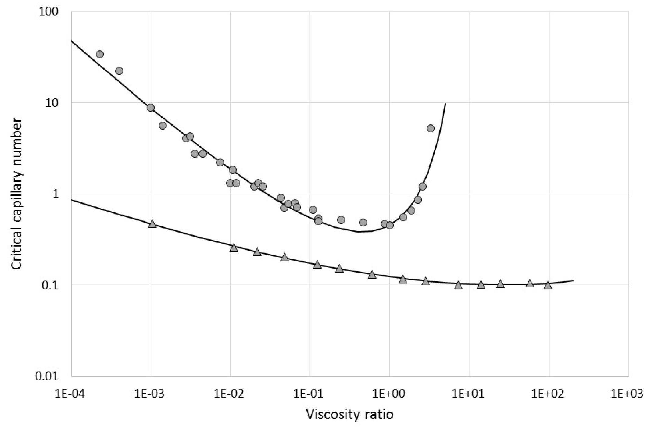
The parameter G has the dimension (1/s). The dimensionless parameter α varies between −1 and 1, and determines the flow type. For α = 1 the flow is a pure 2D hyperbolic (elongational, extensional) flow, while for α = −1 we get a purely rotational flow that does not cause droplet deformation at all. Simple shear is exactly in between these limits (α = 0) and can thus be seen as being composed of equal shares of elongation and rotation. The droplet deformation is fully characterized by two dimensionless numbers. The first one is the so-called capillary number Ca = μ_CRG/σ, where μ_C denotes the viscosity of the continuous phase, R represents the radius of the initial spherical droplet, and σ is the interfacial tension. Physically this number can be interpreted as a measure of the ratio of the deforming hydrodynamic stress (order μ_CG) and the counteracting Laplace pressure (order σ/R), or alternatively as the ratio of the droplet deformation timescale (order = μ_CR/σ) and the process timescale (1/G). The other dimensionless number is the viscosity ratio μ_D/μ_C, henceforth denoted as λ. At sufficiently small values of Ca the droplet reaches a stable deformed shape, but for each value of the viscosity ratio a critical value Ca_C exists above which no stable deformation is possible. Based on systematic experimental work in a four-roll mill, Bentley and Leal [14] have constructed the curves of this critical capillary number versus viscosity ratio for a series of 2D quasi-steady linear flows. De Bruijn [15] has complemented this work by single-droplet studies in simple shear flow, generated in a Taylor-Couette geometry as used also by Grace [13]. These data are reproduced in Figure 1, and analytical correlations for different values of α are provided by Equations (A1) and (A2) in Appendix A. The quality of the fit for the coefficients in

Table A1. Coefficients of Equation (A2), taken from Hill [4].

α	a	b	c	d	e
0	0.935	0.557	−2.150 × 10−5	−1.901 10−3	−0.754
0.2	0.327	0.473	−9.177 × 10−3	−0.248	−1.369
0.4	0.286	0.380	−1.713 × 10−2	−0.292	−1.938
0.6	0.244	0.286	−2.509 × 10−2	−0.336	−2.509
0.8	0.310	0.273	−0.352	−0.435	−3.525
1	0.465	0.454	−0.526	−0.665	−5.259

is illustrated in Figure A1 for α = 0 and α = 1.

For Ca just above Ca_C the droplet typically breaks into two fragments, while for Ca >> Ca_C it stretches into a long fluid thread that breaks into many fragments. For non-Newtonian continuous phases (e.g., non-dilute emulsions or continuous phases with thickeners) the continuous phase viscosity is usually replaced by the apparent emulsion viscosity at the prevailing shear rates (e.g., [9,12,17]).

At first sight it may seem counterintuitive that results for quasi-steady linear flow would be useful for the rapidly changing flows in complex emulsification devices, but it has to be noted that the qualifications “quasi-steady” and “linear” should be interpreted in the context of the length- and time-scales relevant for a droplet deformation process. The final droplet size in many (food) emulsions typically varies between a few and a few tens of micrometers. The relevant length scale is then well below 1 mm and the deformation time scale (order μ_CR/σ) lies well below 0.1 s. Approximating a local flow as “quasi-steady linear” may then be a reasonable approximation in the context of the local droplet behavior. It is a pragmatic assumption, since approaches for droplet deformation in transient flows are more elaborate (e.g., [10,18]) and are not yet widely used in emulsification modelling.

The maximum stable droplet diameter in a 2D quasi-steady linear flow can be calculated from:

$$d_{\mathrm{MAX}}=\frac{2\mathsf{\sigma }\mathrm{C}{\mathrm{a}}_{\mathrm{C}}(\mathsf{\alpha },\mathsf{\lambda })}{{\mathsf{\mu }}_{\mathrm{C}}\mathrm{G}}$$

(2)

This equation is the basis of many semi-empirical models, in which the maximum stable droplet size from the device is assumed to be set by the flow in the “emulsification zone”, e.g., the shear flow within a rotor-stator gap. In fact Equation (2) is rarely considered in detail. Instead many authors assume the mean diameter of interest (e.g., the Sauter mean diameter d₃₂) to be proportional to d_MAX and write:

$$d_{32}=A\frac{\mathsf{\sigma }}{{\mathsf{\mu }}_{\mathrm{C}}\mathrm{G}}$$

(3)

Here A is a dimensionless parameter that has to be fitted to experimental data. It absorbs both the proportionality between d_MAX and d₃₂ and the prevailing value of Ca_C. Additionally, it may empirically compensate to some extent for the differences between 2D and 3D flow, and for deviations from the quasi-steady flow condition. When detailed information about the flow type in the emulsification zone of the device is lacking, this can be a simple and useful approach for a given emulsion-device combination. However, it introduces a hidden λ dependence into the fit parameter A. Moreover it may be that the elongation-shear balance in the local flow changes with process conditions like rotor speed and throughput, which can have a substantial effect on the outcome according to Figure 1. In that case there is no single value for A that covers the whole range of the process conditions even for a given emulsion (fixed λ).

Single-phase CFD may be used to improve the modelling with respect to the issues that originate from the flow complexity, as will be discussed in more detail in the next section. In fact, a detailed flow analysis that provides the relevant parameters for droplet break-up can already be useful to guide geometry optimization of emulsification devices (e.g., number, size and inclination of teeth and slots in toothed rotor-stator mixers) without requiring quantitative droplet size predictions.

3. Droplet Break-Up in 3D Laminar Flows

For 3D linear flows there is no equivalent of Equation (2) available to the best of our knowledge. Indeed, systematic experimental droplet break-up studies in 3D linear flows are much more difficult to design and perform than for the 2D case. A pragmatic way to proceed is to approximate the local 3D flow at each location in the CFD grid by the closest-resembling 2D flow, and then use the correlations in Appendix A to estimate the local value of d_MAX. Hill [4] has suggested a mathematical procedure in which the local coordinate system is rotated such that the local velocity gradient tensor gets as close as possible to a 2D linear flow. In order to quantify the latter condition a merit function is defined as the sum of squares of all components L_ij of the local velocity gradient tensor defined in Equation (1), except L₁₂ and L₂₁. The procedure determines the coordinate system in which the merit function is minimal and transforms the local velocity gradient tensor to that base. We then have, by comparison to Equation (1), L₁₂ ≈ G and α ≈ L₂₁/L₁₂.

For a simulation with many grid cells, as would be needed for industrial rotor-stator devices, this local coordinate system transformation in each cell implies a considerable computational burden. Implementing it for a commercial CFD package will also require user-defined subroutines. We have, therefore, recently updated an alternative that was actually started already in the mid-1990s (see acknowledgments), but not yet implemented in our CFD studies or reported externally. The starting point is the usual split of the velocity gradient tensor into a symmetric and anti-symmetric part, known as the rate-of-strain tensor and the vorticity tensor, respectively:

$$\overline{\overline{D}}=\frac{1}{2}(\overline{\overline{L}}+{\overline{\overline{L}}}^T),\overline{\overline{W}}=\frac{1}{2}(\overline{\overline{L}}-{\overline{\overline{L}}}^T)$$

(4)

Here ^T represents “transposition”, i.e., the exchange of L_ij and L_ji. For the 2D linear flow of Equation (1) we then obtain:

$$\overline{\overline{D}}=\frac{G}{2}\left[\begin{array}{ccc}0& 1+\mathsf{\alpha }& 0\\ 1+\mathsf{\alpha }& 0& 0\\ 0& 0& 0\end{array}\right]\overline{\overline{W}}=\frac{G}{2}\left[\begin{array}{ccc}0& 1-\mathsf{\alpha }& 0\\ \mathsf{\alpha }-1& 0& 0\\ 0& 0& 0\end{array}\right]$$

(5)

We now define the first, second, and third “invariant” of the rate-of-strain tensor as follows [19,20]:

$$\begin{array}{l}{I}_D=Tr(\overline{\overline{D}})\\ I{I}_D=I_D^2-\frac{1}{2}Tr({\overline{\overline{D}}}^2)\\ II{I}_D=\det (\overline{\overline{D}})\end{array}$$

(6)

Here “Tr” denotes the trace operation and “det” is the determinant of the tensor. The same definitions are used for the vorticity tensor. For incompressible fluids I_D = 0. While the name “invariant” suggests that the value is independent of the coordinate system, this is in fact only true for the invariants of the rate-of-strain tensor. We will get back to this point later. For the 2D linear flow of Equation (1) we can derive:

$$I{I}_D=-\frac{1}{4}{G}^2{(1+\mathsf{\alpha })}^2,I{I}_W=\frac{1}{4}{G}^2{(1-\mathsf{\alpha })}^2$$

(7)

These equations can be rewritten to express G and α in terms of the invariants:

$$\begin{array}{ll}\alpha =0& ifI{I}_D=-I{I}_W\\ \alpha =\frac{I{I}_D-I{I}_W+2\sqrt{-I{I}_{D}I{I}_W}}{I{I}_D+I{I}_W}& ifI{I}_D\ne -I{I}_W\\ G=\sqrt{\frac{2(I{I}_W-I{I}_D)}{1+{\alpha }^2}}& \end{array}$$

(8)

The equation for G is valid for all α, but can be simplified for α = 0 to G = √(−4IID) or G = √(4IIW). The invariants can be calculated with a commercial CFD package like ANSYS-Fluent (Canonsburg, PA, USA) from the components of the velocity gradient tensor. However, some useful parameters are already calculated as part of the standard output, namely the rate of strain S and the vorticity magnitude ω. These are directly linked to the above invariants as:

$$S^2=-4I{I}_D,{\mathsf{\omega }}^2=4I{I}_W$$

(9)

Using Equation (9) we can rewrite the Equations (8) as:

$$\begin{array}{ll}\mathsf{\alpha }=0& if{S}^2={\mathsf{\omega }}^2\\ \mathsf{\alpha }=\frac{{(S-\mathsf{\omega })}^2}{S^2-{\mathsf{\omega }}^2}& if{S}^2\ne {\mathsf{\omega }}^2\\ G=\sqrt{\frac{S^2+{\mathsf{\omega }}^2}{2(1+{\mathsf{\alpha }}^2)}}& \end{array}$$

(10)

From Equation (10) the local values of α and G can be readily calculated and combined with the correlations in Appendix A to map the group μ_Cd_MAX/σ = Ca_C/G (or d_MAX itself for given μ_C and σ) across the computational grid for a given viscosity ratio. This requires minimal user coding and little addition to the overall computational effort of the single-phase CFD simulations. Extension to non-Newtonian continuous phases is straightforward, as mentioned in Section 2, provided a correlation is available to link the local value of μ_C to the local value of the shear rate.

The above equations are strictly valid for the 2D linear flow, being based on Equation (1). Computationally, there is no problem to use Equation (10) for a 3D laminar flow. The parameter α remains bound between −1 and 1, and the physical interpretation remains that a value close to 1 characterizes a primarily elongational flow (S² >> ω²) while a value close to −1 points to almost pure rotation (S² << ω²). However, it is not obvious that the result always represents the “closest-resembling 2D flow” in the context of Figure 1. In order to get a better view on how well a given 3D local flow can be approximated by a 2D equivalent we propose to also calculate a dimensionless flow parameter that has been introduced by den Toonder et al. [20]:

$$R_N=\frac{3\det (\overline{\overline{D}})}{{(-I{I}_D)}^{3/2}}$$

(11)

As shown by these authors, R_N varies between −2/√3 for biaxial elongation and 2/√3 for uniaxial elongation, being zero for 2D flow. In fact it is more convenient for our purposes to renormalize R_N such that it varies between −1 and 1, similar to α:

$$R{\prime }_N=\frac{3\sqrt{3}}{2}\frac{\det (\overline{\overline{D}})}{{(-I{I}_D)}^{3/2}}=3\sqrt{6}\frac{\det (\overline{\overline{D}})}{S^3}$$

(12)

A value of R′_N close to zero then indicates that the 2D flow approximation should work, although we cannot suggest a limit for |R′_N| as yet. It is worth noting that during the preparation of the present article we have become aware of a very recent paper by Nakayama et al. [21], in which the parameter R′_N is proposed for characterization of flow patterns in complex mixers.

As was mentioned above the invariants of the rate-of-strain tensor are “objective”, i.e., their value is independent of the coordinate system in which they are evaluated [20,22]. This does not hold for the invariants of the vorticity tensor when comparing coordinate systems that rotate with respect to each other. So, while R′_N is an objective parameter, α and G are not. Objective parameters that incorporate both stretching and rotation have been developed ([22], and references therein), but using these in the present context would be complex and computationally elaborate. In principle the fact that α and G are not objective could lead to “jumps” in their values at the boundary between rotating and stationary mesh parts of a CFD simulation. However, as shown also in the next section, we have not yet observed such behavior in our simulations of rotor-stator devices.

4. Results for a Lab-Scale Toothed Rotor-Stator Mixer (Ultra-Turrax)

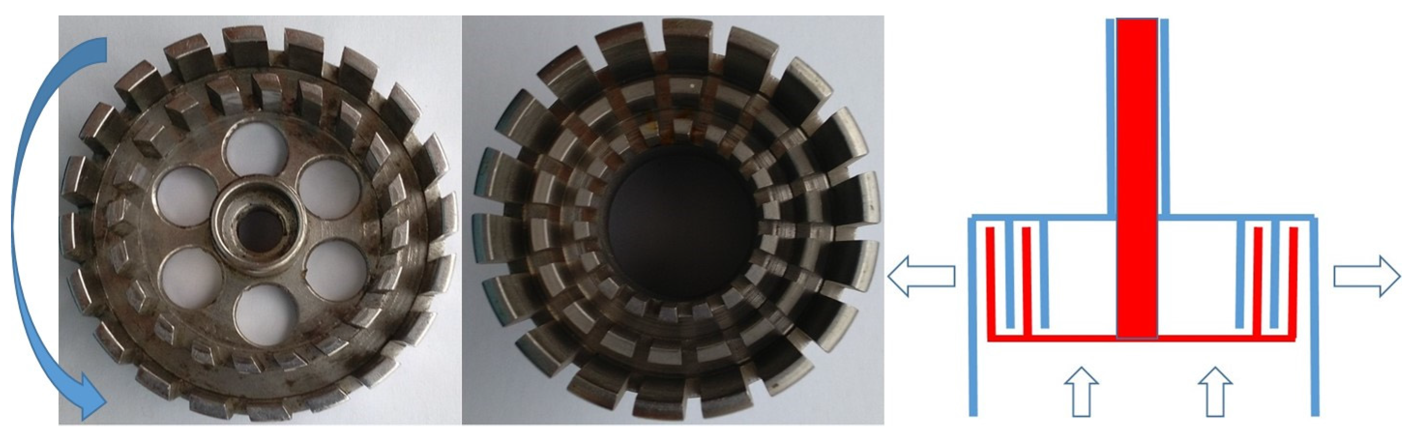
As an illustration we will apply the approach of Section 3 to an IKA Ultra-Turrax T50 (IKA-Werke GmbH, Staufen, Germany) with an S 50N head (laboratory-scale device). The rotor and stator are shown in Figure 2, together with a schematic of their assembly. Important dimensions are listed in

Table 1. Dimensions of the S 50N rotor and stator.

Dimension	Rotor	Stator
Outer diameter (mm)	40	45
Outer diameter middle row (mm)	-	35
Outer diameter inner row (mm)	30	25
Radial tooth thickness (mm)	2	2
Tooth height inner rows (mm)	7	7
Tooth height outer stator row	-	15
Tangential slot width (mm)	2	2
Number of slots	20	18
Entrance hole diameter (mm)	7	-
Gap between adjacent rows (mm)	0.5

.

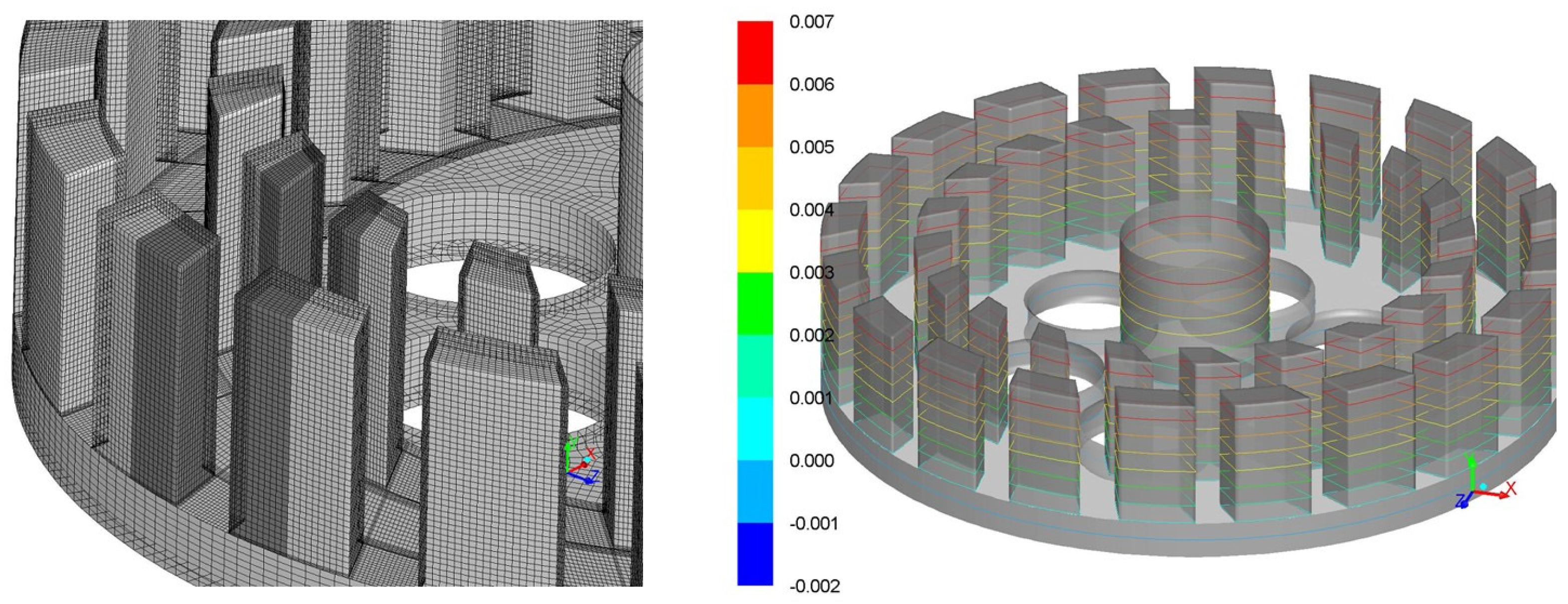
The fluid in the simulations was taken to be Newtonian, with properties that roughly mimic the high-shear behavior of a mayonnaise, i.e., a density of 950 kg/m³ and a viscosity of 0.1 Pas. The simulations have been done with the commercial software FLUENT v.15. The CFD grid consists of three parts: the rotor, the stator, and a substantially larger cylindrical tank into which the mixing head was placed. The rotor was placed in a rotating part of the grid and the other two parts were placed in a non-rotating zone. The mass flow through the head was calculated by integrating the axial velocity over the six circular holes in the base plate of the rotor. The start design of the grid was inspired by the MSc thesis of Ko [23], in which a toothed rotor-stator with one rotor row and one stator row was simulated. His work demonstrated that the cells near the gap walls were more important than those near the center, hence, his use of grid refinement near the walls. Seeking a compromise between accuracy and simulation time, we tested additional variations of structured grids in simplified mill geometries. The grid of one section of the rotor and stator was locally refined (see the darker region in the IKA rotor grid in Figure 3) to check the influence of the calculation grid without facing extremely long calculation times. No significant differences in the local flow variables could be found when comparing the passing of the refined grid sections to the passing of the unrefined sections. A horizontal cross-section of our final grid choice is provided in Figure S1 of the the Supplementary Material.

The equipment used to obtain our results and our approach to the simulations are described below, including the computational time needed for the major steps. The simulations have been performed on a standard PC with a XEON processor with eight core processors and 512 GB memory. We used a similar methodology as Ko [23] and Xu et al. [24] for comparable geometries. The approach was as follows: first, a given simulation was started with a steady multiple reference frame calculation. This calculation took about two days. This then provided the starting point for the second simulation, an unsteady Moving mesh method with a rotation of 0.1° per time step. For a rotational speed of 6000–12,000 rpm, this implied time intervals on the order of 10⁻⁶ s. The results became periodical after about 4–5 rotor teeth had passed a given stator tooth. The unsteady calculation took another 2–3 days. An influence of the six circular holes in the base plate could not be found. For all flow variables second-order schemes have been applied. The gradients have been calculated with the least square cell-based method and the pressure-velocity coupling with the “Pressure Implicit with Splitting of Operator (PISO) ”scheme.

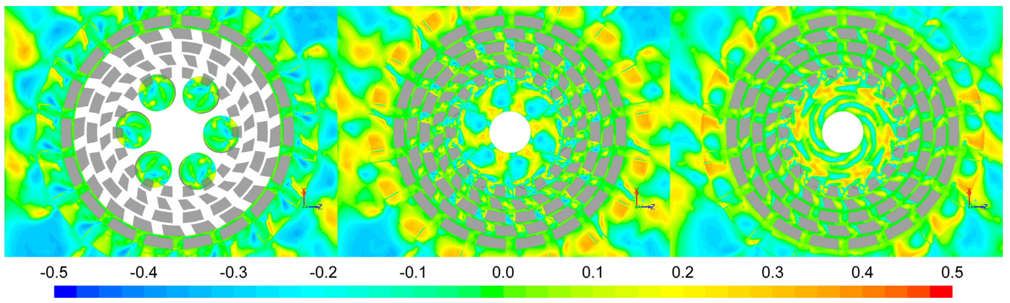
The CFD output at 6000 rpm was visualized as animations of various parameters in several horizontal planes, as indicated in Figure 3, or in a 3D view. An example of the latter is provided in the Supplementary Material. At 6000 rpm the tangential velocity of the rotor is 17.6 m/s and 25.1 m/s at the outer surface of the inner and outer rotor row, respectively. The corresponding Reynolds number for the outer gap is about 120, so a laminar simulation suffices. Our results for the flow field are qualitatively similar to those of Ko [23] and Xu et al. [24], who also used a turbulence model, since their working fluid was water. We have seen that in our simulations the use of a renormalization group (RNG) k-epsilon model with enhanced wall treatment does not give significantly different results.

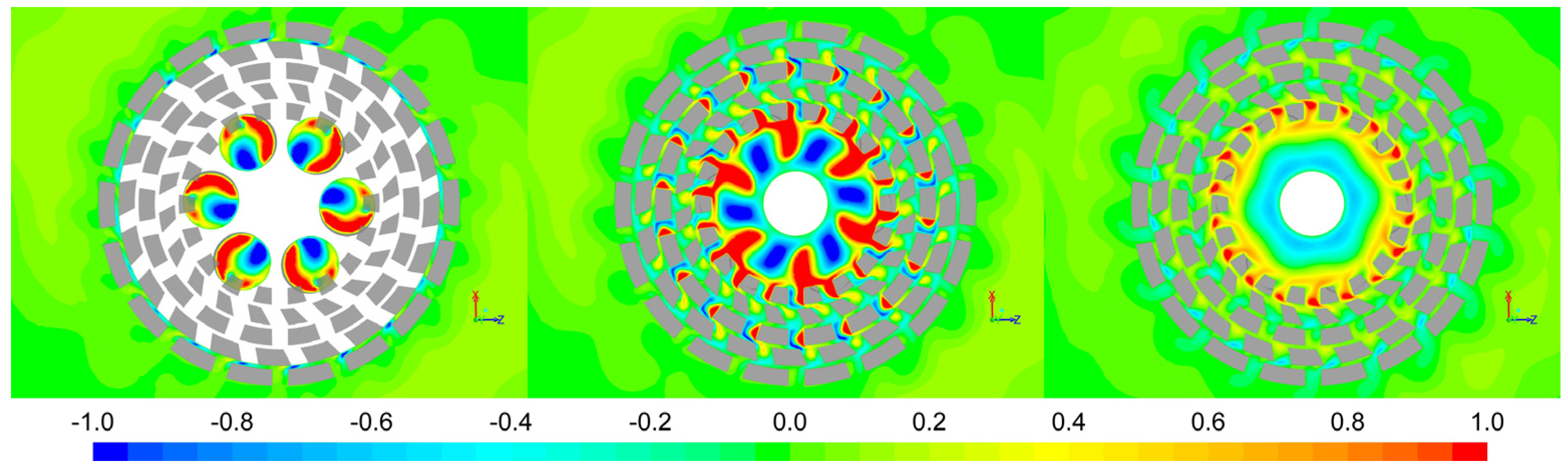
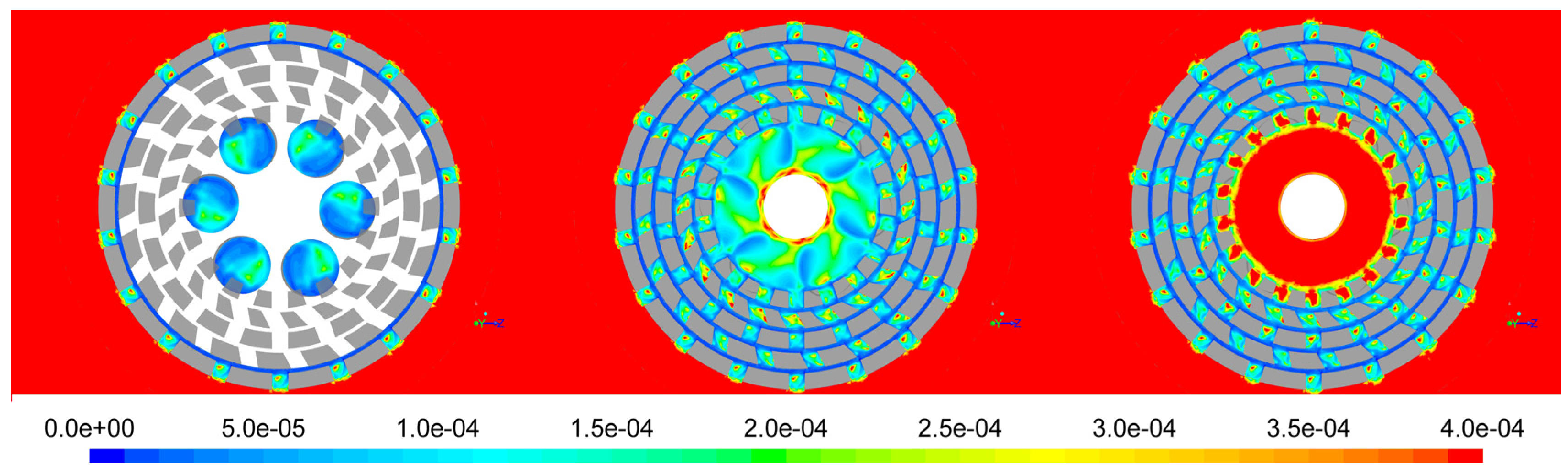
The velocity field (Figure 4 and Figure 5) and the parameters S and ω were available as standard output. The parameters G, R′_N (Figure 6), α (Figure 7), Ca_C/G (Figure 8) and u_RADCa_C/G (Figure 9) were calculated via custom field functions. This increased the overall computing time by 7%–8% compared to a calculation without these additional functions. The most complex parameter is R′_N. When pictures of this parameter are calculated and exported for a sufficiently dense series of time steps to compose an animation, the duration of the simulation can increase up to 30% longer than a calculation without the custom field functions.

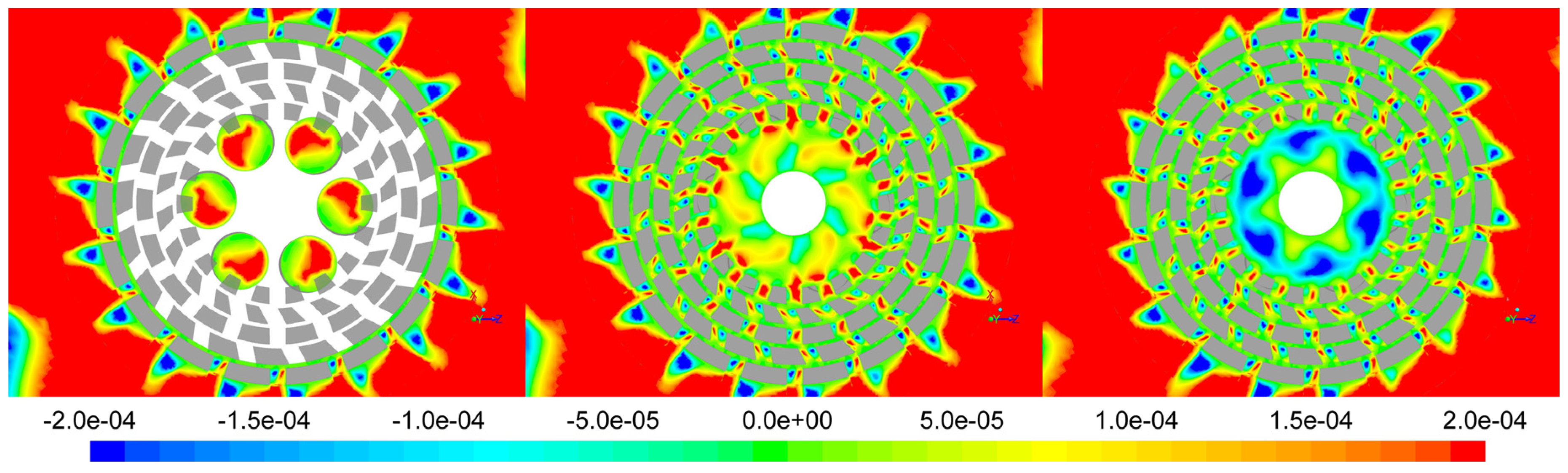
As can be expected, these animations are rich in detail, as illustrated by Video S1 in the Supplementary Material. For our present purposes we will focus on the illustration and assessment of the concepts introduced in the previous sections. Figure 4, Figure 5, Figure 6, Figure 7, Figure 8 and Figure 9 show snapshots of the animations. It is noted that these plots are not fully axisymmetric, due to the fact that the rotor has 20 slots while the stator has 18. In fact, a plot “samples” a series of possible mutual orientations of rotor and stator slots when looking along the tangential direction, which is similar to watching the situation at a given location change in time. The rotor moves counter-clockwise in all plots. At some locations rotor and stator slots are nearly aligned, while at other locations the slots are partly or completely blocked by opposing teeth. It should also be noted that the color scales do not always represent the extremes of the plotted parameter. This interpretation is only applicable when the boundary colors do not appear in the plot. In other cases these boundary colors should be interpreted as “indicated value and larger/smaller” for the upper and lower end respectively. This choice has been made when “color resolution” within the relevant zones of the mixing head is more relevant for the discussion than showing the maximum and/or minimum of the parameter at hand.

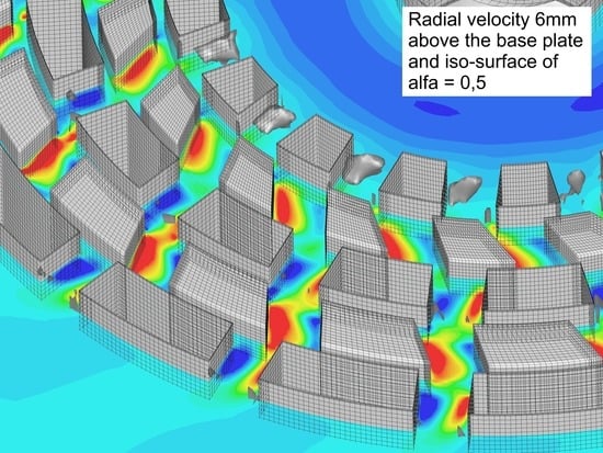
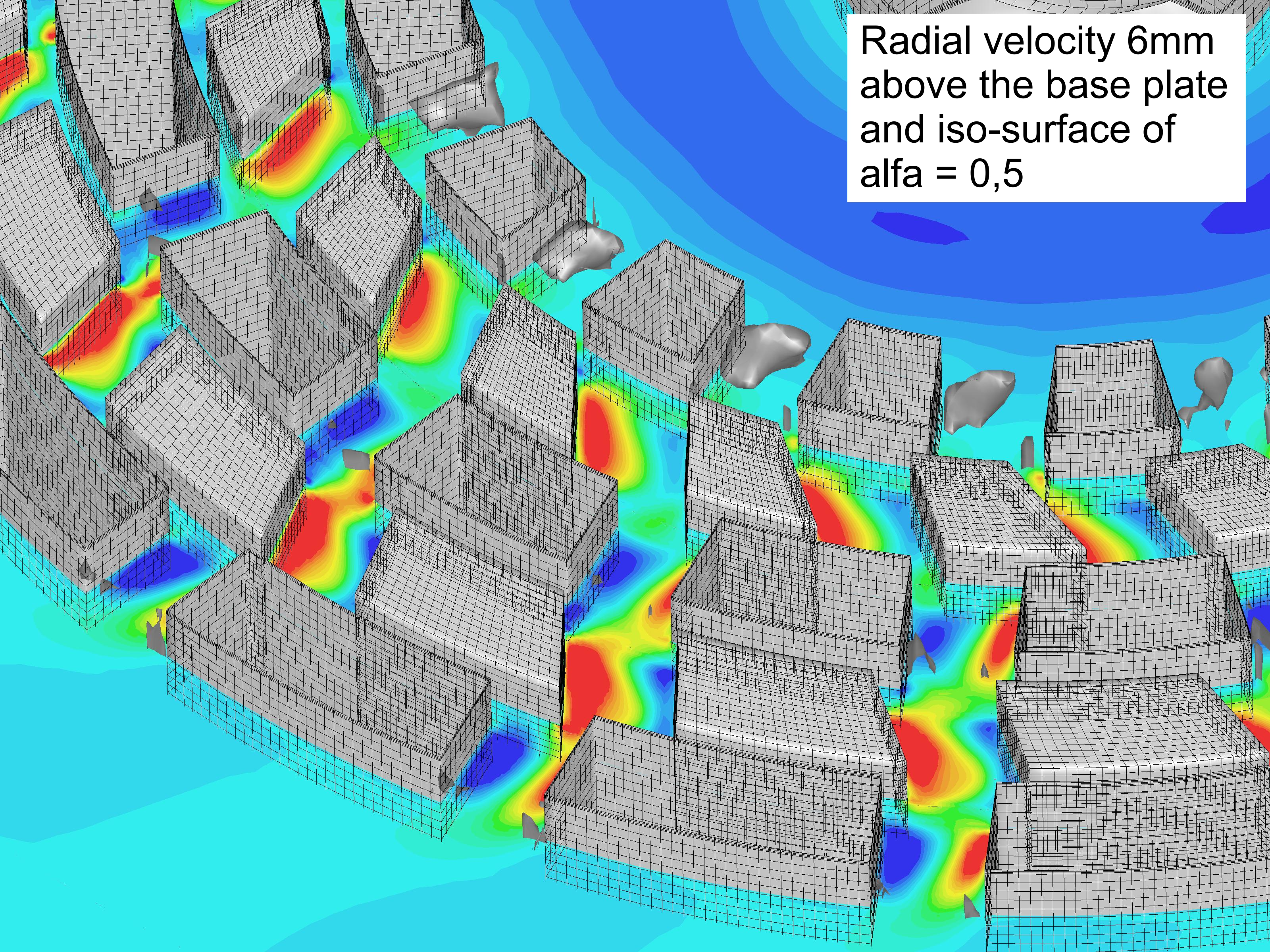
Figure 4 shows the axial velocity components in three horizontal planes. Interestingly the axial flow through the holes in the rotor plate goes in both directions. The most relevant feature for our present purposes is the rapid decrease in the absolute value of the axial velocity when moving radially outward, except close to the tips of the rotor and stator teeth.

Figure 5 shows the radial velocity for the same planes as in Figure 4. Here, a noteworthy feature is the substantial recirculation within all slots, except those of the inner stator row. Additionally, the axial velocity in the outer gap and slots is small compared to the radial and tangential velocity for a large part of the volume of the outer gaps and slots, which suggests a quasi 2D flow. This is supported by the small value of the parameter R′_N in these zones, as shown in Figure 6.

It is noted that, contrary to Figure 4 and Figure 5, we can see the boundaries between different parts of the grid being reflected slightly in Figure 6 (and in plots below that are based on velocity derivatives). Since the value of R′_N does not make a significant step change across these boundaries, we do not think that their visibility is related to the objectivity discussion at the end of Section 3. Rather we conclude that the velocity derivatives are more sensitive to numerical irregularities caused by the rather large aspect ratio of the grid cells adjacent to the boundaries than the velocity components themselves (Figure 4 and Figure 5). Interestingly, the R′_N parameter predicts the flow in the circular holes in the rotor base plate to be rather 2D as well, although the relative magnitude of the velocity components does not readily suggests this. Above the base plates the flow is more 3D in the central part of the mixing head.

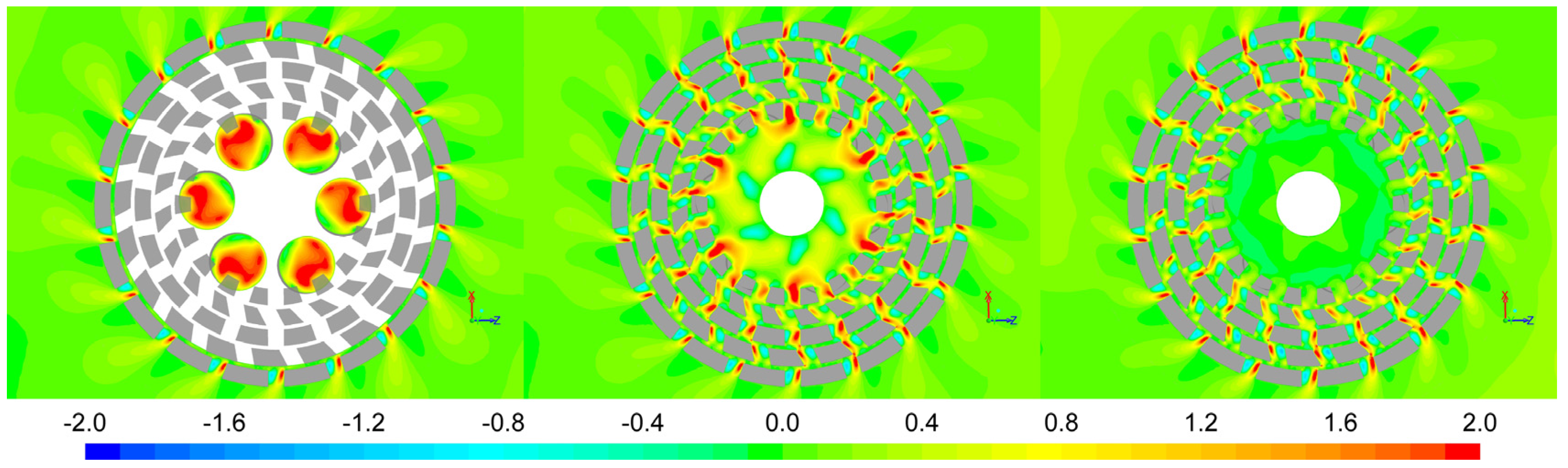
In Figure 7 Equation (9) has been used to calculate the flow parameter α. Here we see that the flow in the gaps between the concentric rows of teeth is basically simple shear, as may be expected from the geometry and the high tangential surface velocity of the rotor. Within the gaps we see both elongational zones and zones with strong rotation. Elongational flow components are also present near tooth edges, as illustrated by the animation in the Supplementary Material. Just outside the stator, “plumes” of elongational flow are seen to emerge from the slots. Of course the interpretation of Figure 7 should be done in conjunction with Figure 6, i.e., if |R′_N| is not small the α values are questionable. The same holds for the other plots that are based on the 2D flow approximation. According to Figure 1, the critical capillary number at a given viscosity ratio decreases with the increasing value of α. However, this does not necessarily imply that the zones with the highest α values in Figure 7 provide the lowest d_MAX. The latter also depends on the corresponding local velocity gradient G. 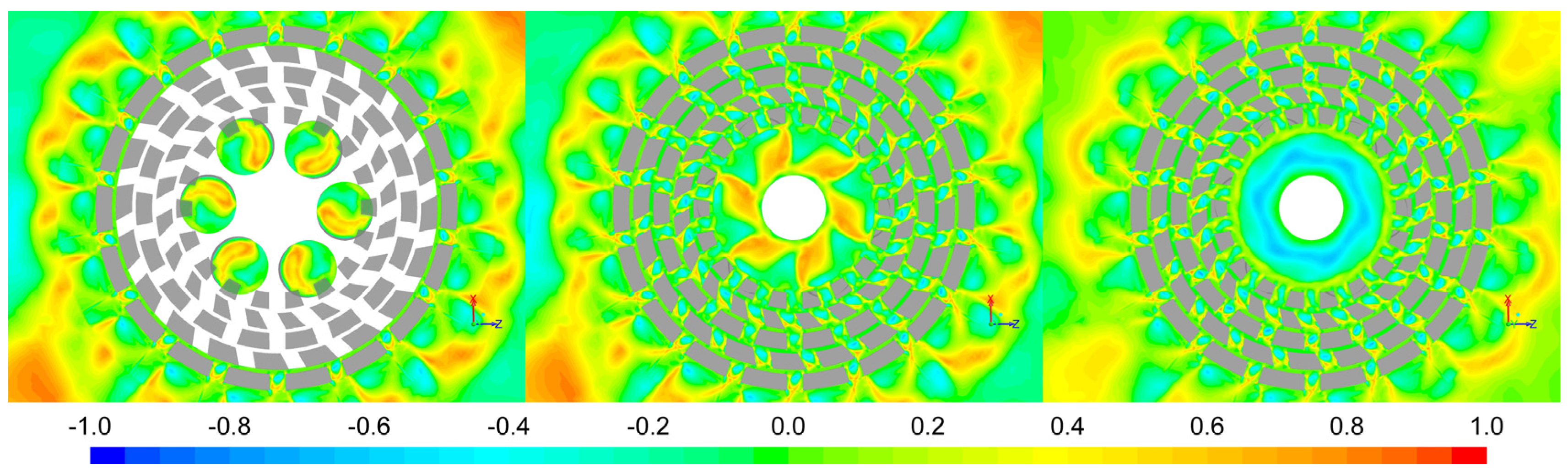Figure 8 shows the group Ca_C/G = μ_Cd_MAX/2σ for a viscosity ratio of unity. Here we see that the smallest values for d_MAX are, in fact, predicted for the outer shear gap, because the local value for G is much higher than in the elongational zones. Surprisingly, we also see small droplets being predicted for the flow through the holes in the base plate. For both low and high viscosity ratios the “emulsification zone” is expected to shift towards the elongational flows in the slots and near the tooth edges. This holds in particular for λ > 4, given the very steep increase in critical capillary numbers with increasing λ in that range for simple shear (Figure 1, α = 0). Indeed experimental data for a toothed rotor-stator reported by Weiss [25] (see also Figure S2 in the Supplementary Material) and for a slotted rotor-stator by Dicharry et al. [26] show that droplet break-up in such rotor-stator geometries remains possible up to high viscosity ratios, although the mean droplet size does increase gradually with λ at given process conditions. The latter is likely due to the fact that the mean diameter is an average of droplets that have followed different streamlines and did not all pass the zones of highest break-up effectivity, as also pointed out by Dicharry et al. [26]. As shown in our animation of “α iso-surfaces” in the Supplementary Material, the volume in which a given α value can be found decreases with increasing α for the Ultra-Turrax, and this will likely be true for toothed/slotted rotor-stators in general.

5. Discussion

Droplet deformation and break-up in emulsification devices is complex, but in batch processes and in-line processes with recirculation we are often mainly interested in the final droplet size distribution, or just a final mean diameter after a sufficiently long processing time. In Section 3 we have proposed a framework to use well-known single-droplet studies (Section 2) for estimating the final maximum stable droplet diameter. Underlying assumptions are that the local flow can be approximated reasonably as 2D and quasi-steady. The parameter R′_N (Equation (11)) has been introduced to characterize the 2D flow approximation, and for the Ultra-Turrax in Section 4 this seems to be valid in the zones that are expected to determine the final droplet size after multiple recirculations. It would be useful to also have an assessment for the validity of the assumption of quasi-steady flow compared to the droplet deformation timescale, for droplets that are already close to d_MAX. This timescale is represented by the group Ca_C/G = μ_Cd_MAX/σ. One option could be to look at the distance that a droplet of size d_MAX travels during its deformation. If this is small compared to the distance over which the local flow changes appreciably, the quasi-steady flow assumption should be locally valid. For a quick view we propose to characterize the travel distance by the product u_RADCa_C/G, since the radial velocity provides a measure of how quickly a droplet traverses a shear gap of a slot. We have calculated this parameter in Figure 9, and see that it is of the order of 0.1 mm or less in the relevant zones. This is small compared to the gap size and the slot dimensions, which may be taken as a rough and easy measure of the distance over which the local flow changes. Figure 9 then suggests that the assumption of quasi-steady flow may not be too bad for droplets close to d_MAX.

We, thus, see that both the 2D assumption and the quasi-steady flow assumption appear reasonable for the zones in which the final droplet size is set. If this is indeed a more general feature of emulsification in rotor-stator devices it suggests an explanation for the apparent success of fitting semi-empirical models based on Equation (3) to the experimental data.

For in-line devices without recirculation it is less obvious that all droplets will pass though the zones with the strongest flow at least once. It may then be an option to monitor d_MAX along a streamline and assume that the smallest value will be the final one for droplets following that path. Doing this for a representative set of streamlines and combining the predicted values of d_MAX with the flow rate along the streamlines, an average droplet size for the emulsion may be estimated. Monitoring the droplet deformation along the streamlines, as done by Feigl et al. [10], and would be more realistic, but would also be a step-change in computational effort.

The framework proposed in this paper only considers droplet break-up, which often suffices for emulsions that are designed for stability, e.g., food emulsions with a long shelf life. Håkansson et al. [27] have shown that coalescence can play a role during the processing of such emulsions, when the adsorption of emulsifiers lags behind the creation of a new interfacial area. However, the latter slows when the final droplet size distribution is approached. Indeed the models of Håkansson et al. [27], with and without coalescence, are quite close with respect to the final mean droplet size.

6. Conclusions

The combination of CFD and population balance models has been explored in the literature as a basis for the modelling of emulsification processes, but for routine industrial use this is still too demanding, computationally. By contrast, semi-empirical models are computationally easy, but based on several strong simplifications, as well as requiring fitting to experimental data. The challenge, thus, is to link a sufficiently detailed flow analysis to the droplet behavior in a way that is both physically relevant and computationally acceptable. In this paper we propose the use of single-phase CFD to map out the local maximum stable droplet diameter within the device, based on well-known academic droplet break-up studies in quasi-steady 2D linear flows. This approach has recently also been used by Rathod and Kokini [12] for bubble size distributions in a co-rotating twin screw mixer, although the details are different. In particular, our implementation includes parameters to assess how good the assumption of quasi-steady 2D flow is locally. Additionally, we use analytical correlations for the required critical capillary number that are valid across a wide viscosity ratio range. These correlations were already available in the literature, but seem to have been largely overlooked. The approach has been applied to a lab-scale Ultra-Turrax, with minimal additional user coding and little increase in computational effort compared to the single-phase CFD simulations of the flow field, as such.

The qualitative trends and order-of-magnitude estimates of our approach can be helpful in the selection and geometry optimization of equipment and for the interpretation of experimental data.