Article

Intelligent Intermittent Production Optimization for Low-Permeability Reservoirs: A Hybrid Physics-Constrained Machine Learning Approach with Dual-Curve Intersection Control

1
China National Petroleum Corporation Changqing Oil & Gas Branch Fifth Oil Production Plant, Xi’an 710020, China
2
State Key Laboratory of Petroleum Resources and Engineering, China University of Petroleum (Beijing), Beijing 102249, China
3
College of Petroleum Engineering, China University of Petroleum (Beijing), Beijing 102249, China
*
Authors to whom correspondence should be addressed.
Processes 2026, 14(9), 1476; https://doi.org/10.3390/pr14091476
Submission received: 8 April 2026 / Revised: 29 April 2026 / Accepted: 29 April 2026 / Published: 1 May 2026
(This article belongs to the Section Petroleum and Low-Carbon Energy Process Engineering)

Abstract

The efficient development of low-permeability reservoirs is critically constrained by severe geological heterogeneity, marginal permeability (<10 mD), and the consequent prevalence of low-productivity wells. Conventional intermittent production management, reliant on empirical fixed-cycle schedules, fails to adapt to dynamic reservoir behavior and wellbore conditions, leading to suboptimal energy efficiency and recovery. This study presents a physics-constrained, data-driven framework for adaptive intermittent production optimization, specifically designed to address the coupled geological-engineering complexities of such reservoirs. The methodology integrates three core innovations: (1) a hybrid flowing bottomhole pressure (FBHP) decline model coupling a “Three-Segment” wellbore pressure calculation with inflow performance relationship (IPR) curves, enabling dynamic characterization of pressure depletion; (2) a shut-in pressure buildup prediction framework combining a physically interpretable dual-exponential recovery mechanism—representing near-wellbore elastic expansion and far-field formation recharge—with a Random Forest Regression algorithm to capture the influence of geological and operational heterogeneity; and (3) a “Dual-Curve Intersection Method” that autonomously determines optimal pumping and shut-in durations by intersecting predicted pressure decline and recovery curves under geological constraints. Field implementation on 15 low-production wells in the Jiyuan Oilfield—a representative low-permeability asset—demonstrated robust performance: average pump efficiency improved from 14.3% to 14.49%, and average single-well electricity savings reached 15.61%. This work establishes a closed-loop intelligent control framework that bridges reservoir geology, wellbore hydraulics, and machine learning, offering a scalable solution for enhancing energy efficiency and production sustainability in low-permeability and unconventional resources.

1. Introduction

The global energy landscape increasingly relies on the efficient exploitation of hydrocarbon resources from low-permeability reservoirs, which are characterized by complex pore-throat networks, marginal matrix permeability (typically below 10 mD), and limited natural energy support [1,2]. These geological attributes result in rapid production decline after initial completion, with a substantial proportion of wells transitioning into a state of low productivity and low operational efficiency. Therefore, the sustainable development of such resources hinges on technologies that can maximize ultimate recovery while minimizing energy intensity, operational costs, and environmental footprint [3]. The Jiyuan Oilfield, a representative low-permeability asset in the Ordos Basin, China, epitomizes these challenges, where severe reservoir heterogeneity, complex fluid–rock interactions, and inadequate formation deliverability collectively contribute to poor pump efficiency and disproportionately high energy consumption per unit of fluid lifted [4].
Intermittent pumping—alternating between production and shut-in periods—has emerged as a widely adopted strategy for managing low-productivity wells in such geological settings [5]. The underlying rationale is to allow bottomhole pressure and fluid levels to recover during shut-in, thereby better aligning artificial lift rates with low formation deliverability [6]. However, traditional intermittent production scheduling has been predominantly empirical, relying on fixed time-based cycles derived from generalized field experience [7]. This static approach fundamentally overlooks the dynamic nature of reservoir depletion, the spatial heterogeneity of geological properties (e.g., permeability distribution, fracture connectivity), and the evolving near-wellbore conditions [8]. Consequently, such schedules often lead to either premature pump-off events—inducing gas interference and excessive mechanical stress—or unnecessarily prolonged shut-in periods that sacrifice potential production [9]. Both scenarios accelerate equipment wear, increase maintenance frequency, and elevate electrical power consumption, ultimately undermining the economic viability of marginal wells [10]. The scientific question is: How to dynamically optimize intermittent production schedules by coupling reservoir geological heterogeneity, wellbore hydraulics, and real-time data? The engineering target is explicitly linked to practical pain points: low pump efficiency (<20%), high electricity consumption per barrel, frequent pump-off events, and inability to adapt to changing reservoir conditions.
The advent of digital oilfield technologies has catalyzed a paradigm shift toward data-driven, intelligent production optimization [11,12]. The integration of Internet of Things (IoT) sensors, high-frequency data acquisition (e.g., continuous dynamometer cards), and advanced analytics offers a transformative pathway beyond empirical control. Central to this intelligent approach is the accurate, real-time estimation of flowing bottomhole pressure (FBHP), which serves as the critical link between reservoir inflow dynamics and wellbore lift performance. While conventional methods for FBHP calculation from fluid level surveys exist, they rely on infrequent manual measurements or simplifying assumptions that compromise accuracy under transient flow conditions [13]. The use of pump dynamometer cards presents a promising alternative for continuous indirect FBHP monitoring, yet its full potential remains underexplored in the context of intermittent production optimization [14]. Autonomous inverse modeling of complex groundwater systems via a physics-integrated large language model multi-agent framework [15]. Comparative research on the performance of three impeller seal clearance structures of pumped-storage units based on improved entropy production theory [16].
Predicting pressure buildup during shut-in periods—a process governed by coupled near-wellbore elastic expansion and far-field formation recharge—is equally essential for determining optimal shut-in durations [9]. Traditional analytical models often fail to capture the complex recovery behavior influenced by wellbore storage effects, reservoir heterogeneity, and multiphase flow [17,18]. Recent advances in machine learning, particularly ensemble methods such as Random Forest and Gradient Boosting, have demonstrated strong capabilities in modeling nonlinear relationships from high-dimensional operational data. Studies have successfully applied these techniques to production forecasting [19], induced seismicity risk assessment [20], and estimated ultimate recovery (EUR) prediction with physical constraints [21]. However, the potential to learn nuanced patterns of pressure recovery—incorporating both static geological attributes and dynamic production states—has not been fully leveraged for intermittent production optimization.
To address these interconnected challenges, this study proposes a closed-loop intelligent framework for adaptive intermittent production optimization in low-permeability reservoirs. The research rests on three foundational pillars that integrate geological understanding, wellbore hydraulics, and machine learning:
(1)
A dynamic FBHP decline model coupling a “Three-Segment” wellbore pressure calculation with inflow performance relationship (IPR) curves, enabling physically consistent characterization of pressure depletion during production;
(2)
A hybrid data-physics model for shut-in pressure buildup prediction, combining a dual-exponential recovery mechanism—physically representing near-wellbore elastic expansion (fast recovery) and far-field formation recharge (slow recovery)—with Random Forest Regression to capture the influence of geological heterogeneity and operational history;
(3)
A novel “Dual-Curve Intersection Method” for intelligent decision-making, autonomously determining optimal pumping (Ton) and shut-in (Toff) durations by intersecting predicted FBHP decline and recovery curves under geological constraints.
By synergistically integrating mechanistic understanding with machine learning, this work advances beyond static experience-based control toward a responsive, well-specific, and geologically informed optimization paradigm. The framework is validated through field implementation on 15 low-productivity wells in the Jiyuan Oilfield, with results demonstrating significant improvements in energy efficiency and operational stability.

2. Geological Setting

The Jiyuan Oilfield, located in the Ordos Basin of central China, serves as the field laboratory for this study. The Ordos Basin is a large intracratonic basin characterized by extensive low-permeability and tight sandstone reservoirs. The primary producing intervals in the study area are the Triassic Chang 6–Chang 8 members, which represent delta-front to shallow-lacustrine depositional environments.
Reservoir characterization reveals matrix permeability ranging from 0.1 to 5.0 mD, with an average of 0.8 mD; porosity between 6% and 14%, averaging 9.5%; pore-throat radii predominantly in the 0.1–1.0 μm range, exhibiting strong heterogeneity; fracture development varying spatially, with natural fractures primarily oriented NE-SW; formation pressure coefficient ranging from 0.75 to 0.85, indicating underpressured conditions; crude oil properties: viscosity of 2–8 mPa·s, density of 0.82–0.86 g/cm3, with varying water cut across the field.
These geological characteristics collectively result in rapid production decline, poor formation deliverability, and strong sensitivity to operational practices. The 15 wells selected for this study span three distinct reservoir sub-zones within the Chang 8 member, capturing variations in permeability, fracture intensity, and water cut to ensure the robustness of the developed methodology.

3. Methodology

3.1. Data Acquisition and Preprocessing

The proposed intelligent intermittent production optimization framework relies on multi-source data acquired from 15 low-production wells in the Jiyuan Oilfield. Table 1 summarizes the data sources, sampling frequencies, and key parameters utilized in this study. It is noted that the well’s pumping speed is 1.5–2.5 strokes per minute, and the sampling rate is 1 min, giving approximately 5–6 data points per stroke cycle. A window size of 5 effectively removes high-frequency noise (>0.5 Hz) from electrical and mechanical sources while preserving the fundamental pumping frequency. A sensitivity analysis (window sizes 3, 5, 7, 10) confirmed that size 5 minimizes RMSE against a manually cleaned reference signal. For cross-well engineering applications, we now provide a practical guideline: “window size = (sampling rate in samples per minute)/(pumping speed in strokes per minute) × (0.5 to 1.0)”. For wells with different pumping speeds, the window size should be scaled proportionally.
Raw high-frequency dynamometer data undergo the following preprocessing steps:
(1) Noise filtering: A moving average filter (window size = 5) removes high-frequency noise from load and position signals;
(2) Stroke feature extraction: Wave equation solution (Section 3.2.1) extracts effective stroke length, pump load, and displacement per stroke cycle;
(3) Temporal aggregation: Stroke-level features are aggregated into hourly averages to align with shut-in event records;
(4) Normalization: All input features are scaled to zero mean and unit variance for machine learning compatibility.
The final dataset comprises 320 shut-in buildup events across 15 wells, with 70% randomly selected for training and 30% for validation.

3.2. Physics-Based FBHP Decline Model

3.2.1. Surface-to-Pump Dynamometer Card Conversion

The complete mathematical model for a rod pumping system with multi-stage rods includes the wave equation, boundary conditions, and initial conditions [22,23]:
2 u ( x , t ) t 2 = a 2 2 u ( x , t ) x 2 c u ( x , t ) t u x , t | x = 0 = S t , F x , t | x = 0 = F t , u x , t | x = L = S 0 t F x , t | x = L = F 0 t u ( x , t ) | ( 0 x L , t = 0 ) = 0 , F ( x , t ) | ( 0 x L , t = 0 ) = 0 F r d ( t ) = F r + 1 u ( t ) , S r d ( t ) = S r + 1 u ( t )
where x is the downhole depth from the polished rod; a is the velocity of the stress wave in the sucker rod; u(0,t) and F(0,t) are the displacement and load functions at the polished rod, respectively; c is the damping coefficient; Fr(t) and ur(t) are the load and displacement at the bottom of the r-th grade rod at time t, respectively.
The separation of variables method is used to solve the wave equation, obtaining its analytical solution [24]:
u x , t = σ 0 x 2 E A + v 0 2 + n = 1 O n x cos n ω t + P n x sin n ω t  
F ( x , t ) = E A [ σ 0 2 E A + n = 1 O n ( x ) cos n ω t + P n sin n ω t ]  
where EA is the rod stiffness, defined as the product of Young’s modulus, E, and the rod’s cross-sectional area, A.
The damping coefficient is solved iteratively. The effective stroke S e is extracted as
S e = S C S D
where Sc is the computed stroke from the wave equation solution, and Sd is the deformed stroke due to rod stretch (i.e., the elastic elongation of the rod string under load).

3.2.2. Three-Segment FBHP Calculation

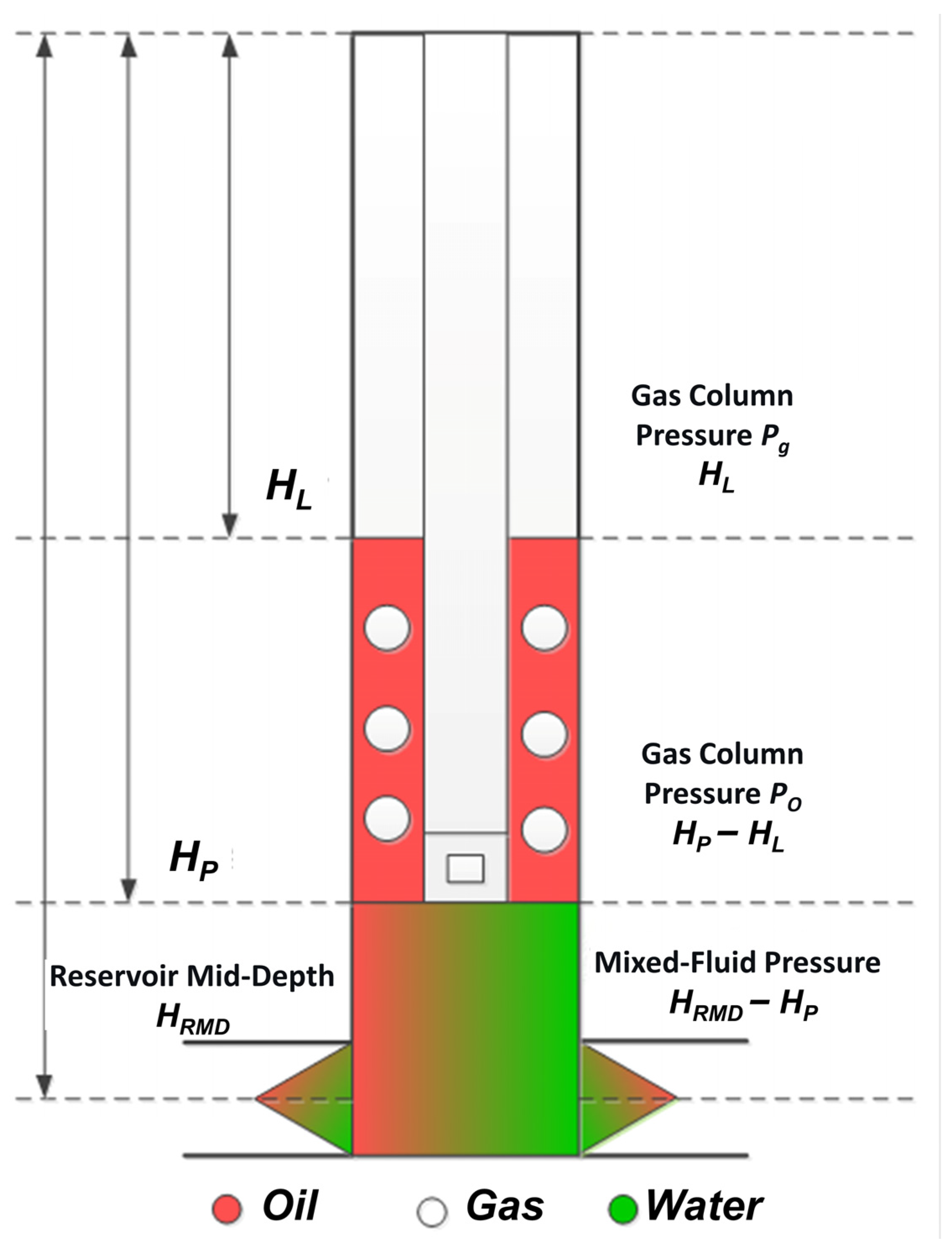
During normal production, fluids in the pumping wellbore are divided into three segments: gas column, oil column, and mixed liquid column [25]. Bottomhole pressure equals the sum of their pressures:
Pwf = Pg + Po + Pow
where Pwf is the bottom pressure. Pg, Po, and Pow, which are the gas column pressure, oil column pressure, and mixed liquid column pressure, respectively.
Gas column pressure (above fluid level) is calculated as a static gas column [26]:
Pg = Pc + (Pc + 0.1) × Hl/12,500
where Pc is the casing pressure, and Hl is the dynamic fluid level depth.
Oil column pressure (from fluid level to pump intake) assumes pure oil due to gravity segregation [27]:
P o =   ( H b H l ) γ o l n ( 1 + b P g a + b P o ) 100 b
where Hb is the pump depth, Hl is the fluid level depth, γ o is the oil specific gravity, and a and b are the empirical gas coefficients.
Mixed liquid column pressure (below pump intake) accounts for oil–water–gas mixtures:
P o w =   ( H R M D H P ) F g c γ w f w 100 +   ( H R M D H P ) F g c ( 1 f w ) γ o 100 b P o w ln   [ 1 + b P o w a + b ( P g + P o ) ]
where HRMD is the mid-reservoir depth, and Hp is the pump intake depth. The gas void fraction ϕg and correction factor Fgc = 1 − ϕg are determined from gas velocity calculations based on the gas state equation [28].
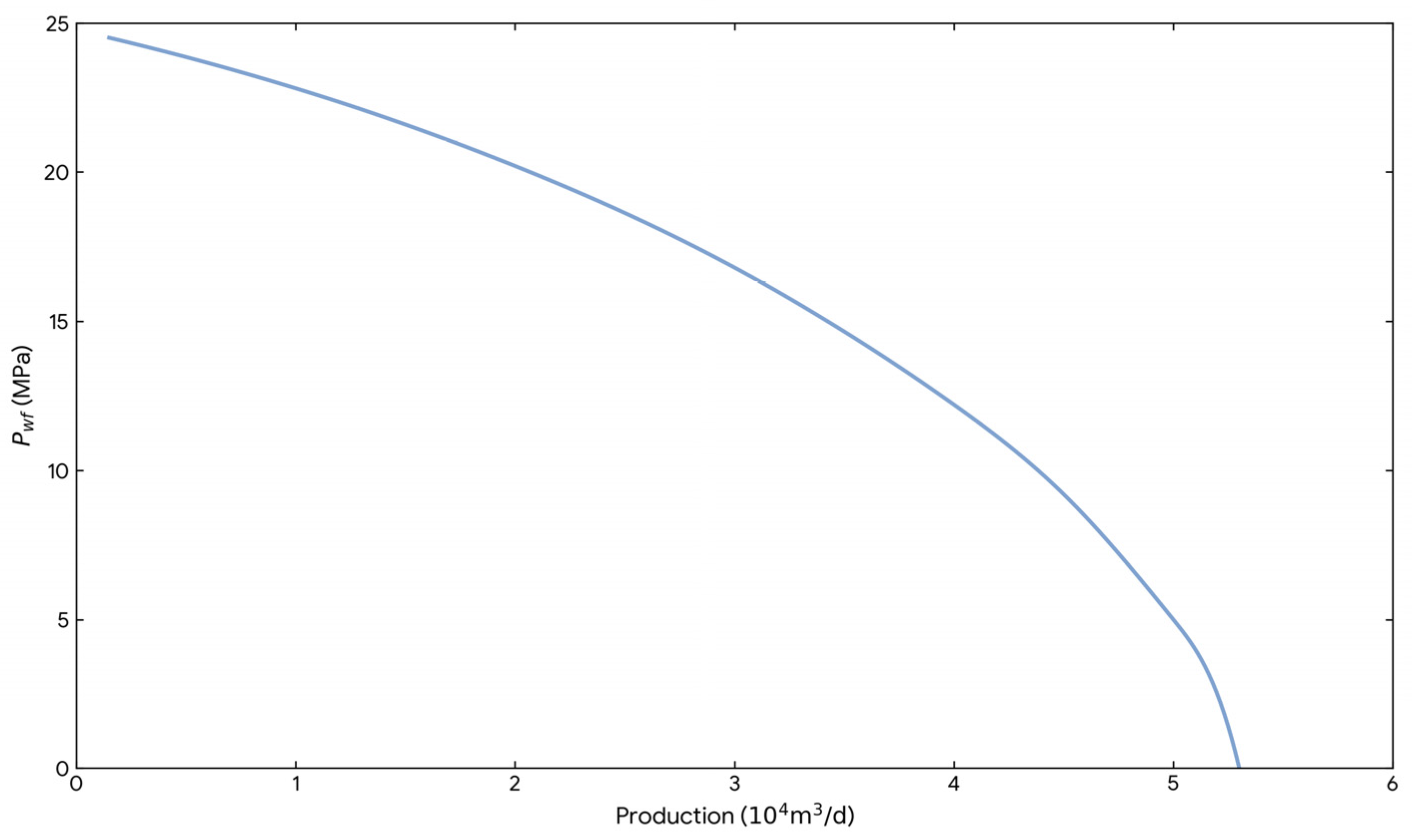
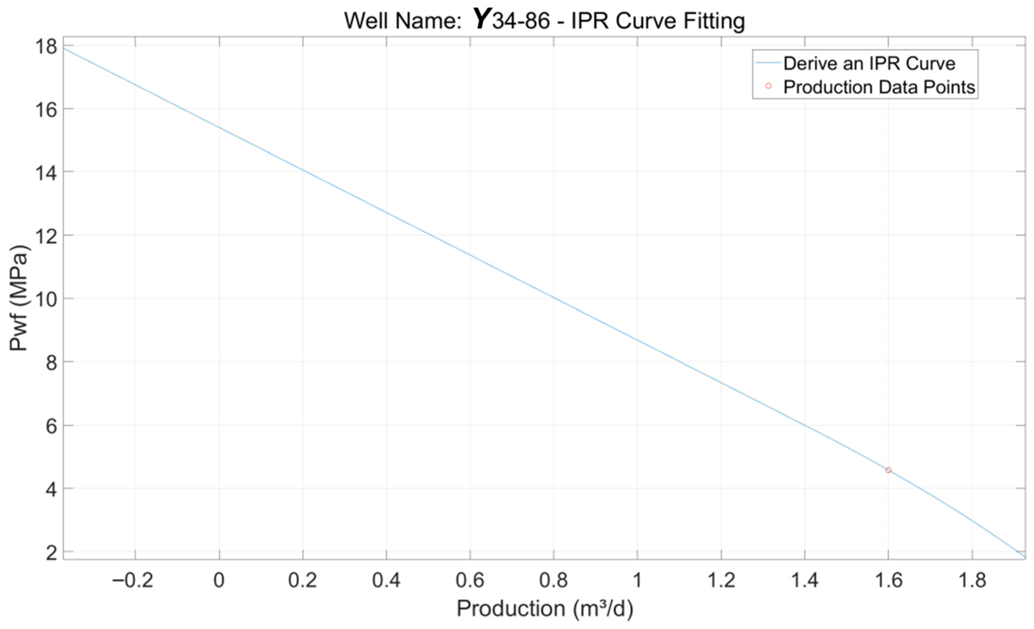
Figure 1 shows a typical IPR curve for a well, illustrating the relationship between production rate and FBHP. Figure 2 depicts the three-segment fluid column in the wellbore.

3.2.3. Dynamic Prediction Numerical Algorithm

Based on mass conservation, an iterative solution is performed with time step Δt [29,30]: ① Initialization: Based on shut-in stable FBHP Pwf0, invert the initial dynamic fluid level height H0 via the wellbore model. ② Iterative Calculation: Calculate formation inflow rate Qin (Pwf) under current FBHP Pwf (via IPR model). Calculate current pump displacement Qpump ( Q p u m p = 1440 A p S N η p ). Calculate annulus liquid column height change Δh ( Δ h Δ t = Q 0 [ P w f ( h , t ) ] Q p i m p [ P s ( h , t ) ] 0.25 π ( d c i 2 d t e 2 ) ). Update fluid level height Hnew = Hold + ΔH. Based on new Hnew, recalculate FBHP Pwf_new using the “Three-Segment Method.”③ Loop and Output: Repeat iterative calculation until the prediction time ends, outputting curves of dynamic fluid level and FBHP versus time. The pseudocode clearly outlines each step of the iterative FBHP and fluid level prediction procedure. The pseudocode is presented as follows (Algorithm 1):
Algorithm 1: Dynamic prediction of FBHP and fluid level
Input:
   - Initial shut-in FBHP P_wf0
   - Well parameters (pump depth H_b, casing/tubing dimensions, etc.)
   - IPR curve coefficients
   - Time step Δt
   - Total prediction time T
Output: Time series of FBHP and fluid level depth
1:   Initialization:
       H_current ← invert P_wf0 using the Three-Segment wellbore model (Equations (5)–(8))
2:   for t = 0 to T step Δt, do
3:           Compute formation inflow rate q_in(P_wf) using the IPR model
4:           Compute current pump displacement:
                   q_pump = 1440 × A_p × S × N × η_p
5:           Compute annulus liquid column height change:
                   ΔH = (q_in−q_pump) × Δt/(0.25 × π × (d_ci2−d_te2))
6:           Update fluid level depth:
                   H_new = H_current + ΔH
7:           Recompute FBHP P_wf_new using the Three-Segment Method (Equations (5)–(8))
8:           Store (t, P_wf_new, H_new)
9:         H_current ← H_new
10: end for
11: Return the stored time series.
There are three reasons for not using machine learning for FBHP decline: (i) interpretability—the three-segment model decomposes pressure into gas, oil, and mixed liquid columns with clear physical meaning; (ii) data efficiency—transient decline data are sparse (320 events across 15 wells); (iii) extrapolation—physics models remain valid outside training ranges. To verify necessity, we trained a Random Forest model on the same dataset. The RF achieved an MAE of 8.7% vs. 4.3% for our physics model, occasionally produced unphysical pressure increases, and required >800 samples for stable performance, whereas the physics model worked with only 50 samples. These results confirm that a physics-based decline model is essential for this task.

3.3. Hybrid Machine Learning Model for Shut-In Pressure Buildup

3.3.1. Dual-Exponential Recovery Mechanism Model

Based on pressure buildup physics, the recovery curve is expressed as a superposition of two exponential processes [31]:
P ( t ) = P 0 + ω Δ P ( 1 e r 1 t ) + ( 1 ω ) Δ P ( 1 e r 2 t )
(1) First Stage (Fast Recovery, weight ω): Reflects elastic expansion near the wellbore and release of local fluid compressibility, controlled by factors like pump depth, wellbore storage, and water cut; (2) Second Stage (Slow Recovery, weight 1 − ω): Reflects the recharge process from the deep formation to the wellbore, influenced by factors like formation permeability, oil viscosity, and drainage radius. Parameters (P0, A, k1, k2, ω) of this model have clear physical meanings, enhancing model interpretability.

3.3.2. Random Forest for Parameter Prediction

Random Forest, an ensemble learning method, constructs multiple decision trees and aggregates their predictions for robust regression tasks [19,32]. It employs bootstrap sampling and random feature selection to enhance diversity and generalization.
(1) Algorithm Principle and Working Mechanism
The core mechanisms of Random Forest include bootstrap sampling and random feature selection. During model training, the algorithm draws multiple subsamples with replacement from the original dataset, each used to train a decision tree [33]. At each node split within a tree, only a random subset of all features is selected for the optimal split, thereby enhancing model diversity and generalization [20]. Finally, the regression results of all decision trees are averaged as the Random Forest prediction output:
y ^ = 1 N t r e e i = 1 N t r e e T i ( x )
where y ^ is the predicted value, Ntrees is the number of decision trees, and Ti(x) is the output of the i-th tree.
(2) Feature Engineering and Input-Output Design
This study selects eight categories of easily obtainable static and dynamic parameters that significantly influence the pressure recovery process as model inputs [34]: ① Static Parameters: pump depth, mid-reservoir depth [35]; ② Dynamic Parameters: water cut, pump efficiency, stroke length, pumping speed, pre-shut-in opening duration [36]; ③ Production State Parameters: FBHP before shut-in, dynamic fluid level depth. The outputs are the five key parameters of the dual-exponential recovery model: initial pressure P0, pressure buildup amplitude A, fast recovery coefficient k1, slow recovery coefficient k2, and fast recovery weight ω.
The dominant influence of pump depth and pre-shut-in opening duration on the recovery rates (r1,r2) reflects the underlying physics of low-permeability reservoirs. In such formations, wellbore storage dominates the early pressure response, while the limited matrix permeability makes the slow recharge rate (r2) highly sensitive to the duration of prior production (which governs the radius of depletion). The strong impact of water cut on ΔP and ω highlights how multiphase flow alters the reservoir’s effective compressibility and near-wellbore relative permeability—a key characteristic of mature low-permeability fields where water breakthrough is common. These findings confirm that the model captures essential reservoir dynamics rather than spurious correlations. For the model design, pump depth and pre-shut-in duration have been deliberately included as direct inputs, while excluding features that are collinear or lack physical causality. Their high importance validates this choice.
(3) Model Training and Hyperparameter Tuning
Historical shut-in buildup data from 15 wells (totaling 320 samples) are used to construct the training set. The 70/30 split is standard for small to moderate datasets (320 samples), ensuring sufficient training samples (224) while retaining a representative test set (96). Grid search combined with 5-fold cross-validation is employed for hyperparameter optimization. The final model configuration is number of decision trees Ntrees = 200; maximum tree depth max_depth = 15; minimum samples per leaf min_samples_leaf = 2; min_samples_split = 5; feature random selection ratio max features = n f e a t u r e s .
(4) Feature Importance Analysis
To further enhance model interpretability, Gini importance is used to evaluate the contribution of each input feature to pressure recovery parameter prediction [37]. Analysis results show that pump depth and pre-shut-in opening duration have the most significant impact on recovery rate parameters k1, k2; water cut and pump efficiency mainly affect pressure buildup amplitude A and weight parameter ω; mid-reservoir depth and stroke length have relatively smaller contributions but remain indispensable in the overall model. ① Pump depth: Deeper pumps increase wellbore storage volume, prolonging the fast recovery stage (higher r1 sensitivity) because more fluid must be redistributed before formation recharge dominates. ② Pre-shut-in opening duration: Longer production prior to shut-in creates a larger pressure drawdown and deeper near-wellbore depletion, which directly affects the initial buildup slope. ③ Water cut: Higher water cut changes relative permeability, reduces gas interference, and alters the fast-to-slow recovery balance (affects weight ωand amplitude ΔP). ④ Pump efficiency: Lower efficiency indicates pump-off or gas interference, which reduces the effective drawdown and thus changes the pressure buildup amplitude.
(5) Model Verification and Performance Evaluation
The model’s pressure buildup prediction results on 15 validation wells are shown in Table 2. The overall prediction mean absolute error (MAE) is less than 5%, and the coefficient of determination R2 > 0.95. Especially during the initial buildup phase (<2 h) and stable phase (>6 h), the model prediction curves highly match with measured data, validating the effectiveness and applicability of the Random Forest Regression algorithm in predicting wellbore pressure buildup dynamics. The averaged metrics across the five folds are mean absolute error (MAE) of 4.35% (±0.21%); root mean square error (RMSE) of 0.38 (±0.03), and coefficient of determination (R2) of 0.949 (±0.008). These values are highly consistent with the independent test set results (MAE = 4.3%, RMSE = 0.35, R2 = 0.95), confirming that the model does not overfit and generalizes well. Additionally, the results presented in Table 2 (pressure buildup prediction errors) correspond to a single hold-out test set (30% of the data, randomly selected). This test set was not used during hyperparameter tuning or any other training step, thus providing an unbiased estimate of model performance on unseen data. Moreover, the five-fold CV results (reported as averages ± standard deviations) were used only for hyperparameter selection (grid search) and internal validation.
Here, both a five-fold CV and independent test set results have been provided. The final performance assessment is based on the independent test set, which is the most rigorous estimate of generalization. The CV results serve as an internal consistency check. Our dataset comprises 320 shut-in events from 15 wells. These events are not independent in a statistical sense (multiple events per well). A random 70/30 split across events still preserves well-level diversity in both training and test splits, and we further ensured that events from the same well appear in both splits only after confirming that reservoir/operational conditions varied sufficiently within each well. Moreover, we repeated the random split three times with different random seeds and obtained nearly identical test metrics (variation <0.2% in MAE), indicating that the single split is representative. The five-fold CV results (R2 = 0.949 ± 0.008) are virtually identical to the test set performance (R2 = 0.95). This close agreement demonstrates that the model’s performance is stable and not an artifact of a particular split. Therefore, the single test split is sufficient for reporting final performance, especially when complemented by CV metrics.

3.3.3. Pressure Buildup Calculation Flowchart

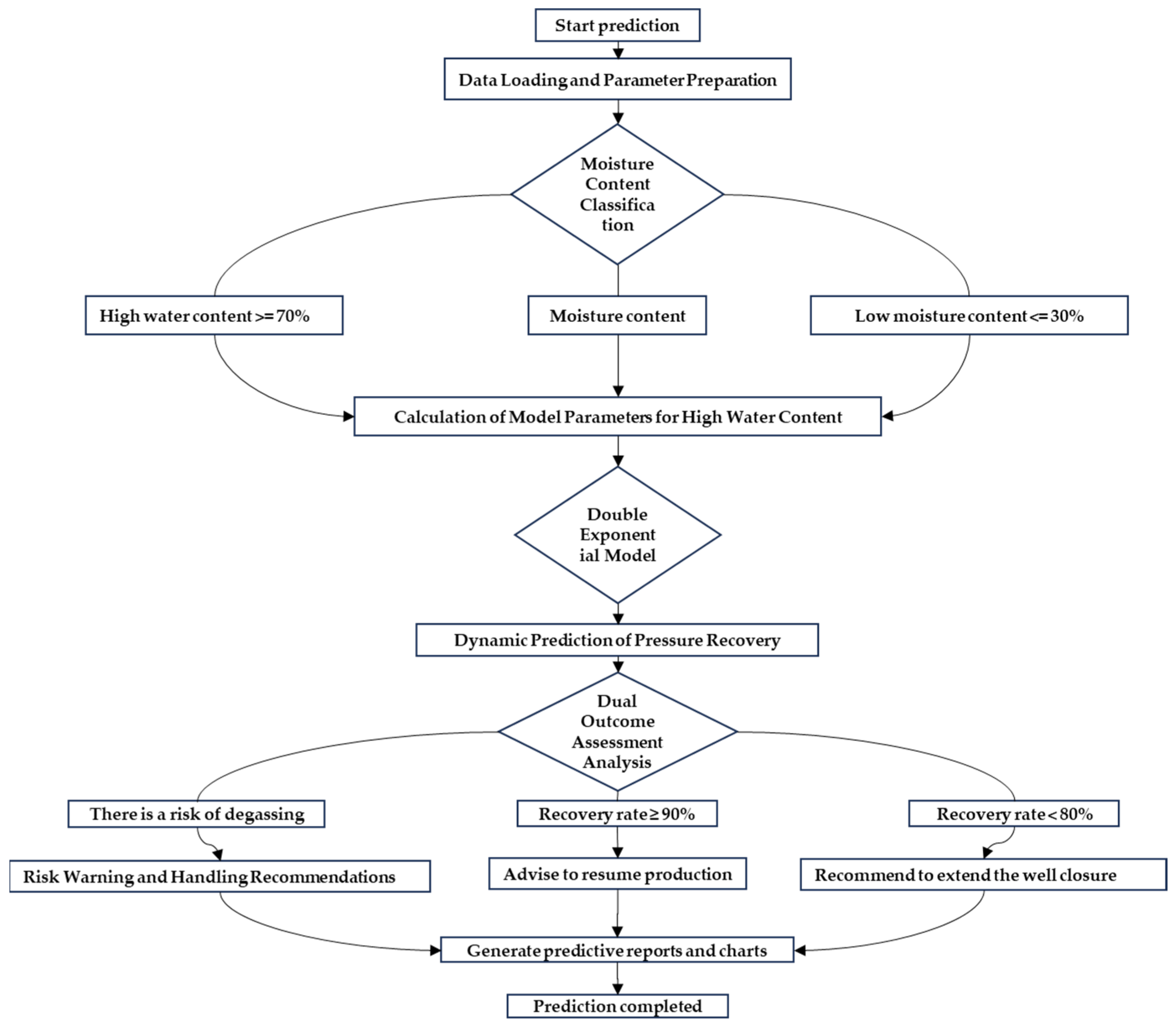
The process starts with “Data Loading and Parameter Preparation,” providing foundational data for subsequent analysis. A key decision point is the “Water Cut Classification Judgment,” which directs the flow based on the current reservoir water cut. If water cut ≥ 70%, it proceeds to the “High Water Cut Model Parameter Calculation” step for specialized processing. If the water cut is between 30 and 70% or <30%, it directly enters the next core step: “Dual-Exponential Model Prediction.” This core mathematical model is used to predict the pressure recovery after shut-in over time. The main steps include data loading, water cut classification judgment, model parameter calculation, and dual-exponential model prediction. The flowchart is shown in Figure 3.
It is noted that the physical constraints embedded in the training process: (1) the dual-exponential recovery function (Equation (9)) imposes a physics-based structure (monotonic recovery to a finite asymptotic pressure); (2) during training we enforce hard constraints—positivity of r1, r2, ΔP and 0 ≤ ω ≤ 1; any prediction violating these bounds is clipped to the nearest physically plausible range; (3) the Random Forest is used only to estimate the five physically meaningful parameters of the dual-exponential model, not to directly predict pressure in a black-box manner.

3.4. Dual-Curve Intersection Decision Algorithm

Building on the accurate FBHP decline and recovery prediction capabilities established earlier, this study further proposes the “Dual-Curve Intersection Method” intelligent decision-making algorithm [38]. The core idea is to find the optimal intersection point between the pressure buildup curve and the FBHP decline curve in the time-pressure coordinate system, thereby maximizing cycle liquid production or minimizing lifting energy consumption per ton of liquid, subject to engineering hard constraints [39]. Specifically, the buildup model predicts the FBHP recovery value corresponding to different shut-in durations, Toff (Curve A). The decline model predicts the FBHP decline value corresponding to different opening durations, Ton, starting from the recovery endpoint pressure (Curve B) [40]. Under the constraints of FBHP not falling below bubble point pressure and the total cycle not exceeding 24 h, the optimal pair of shut-in and opening durations (Toff, Ton) is solved through intersection optimization [41]. This method fundamentally changes the traditional experience-dependent intermittent production scheduling mode, providing a new decision-making framework for the intelligent, efficient, and adaptive control of low-production wells [42].
Based on the high-precision FBHP decline and recovery prediction models constructed earlier, this study proposes the “Dual-Curve Intersection Method” intelligent decision-making algorithm. The core idea is to find the optimal intersection point between the pressure buildup curve and the FBHP decline curve in the time-pressure coordinate system, achieving cycle liquid production maximization or lifting energy consumption per ton of liquid minimization under engineering hard constraints [43]. Specific steps are as follows:
(1) Curve Plotting: Curve A (Recovery Curve): Predicts the FBHP recovery value, Prec (Toff), corresponding to different shut-in durations Toff starting from the current moment; Curve B (Decline Curve): Predicts the FBHP decline value Pdrop (Ton) corresponding to different opening durations Ton, starting from the recovery endpoint pressure [44]. (2) Intersection Optimization: Under the condition Prec (Toff) = Pdrop (Ton), optimize to obtain the optimal pair (Toff, Ton) [45]. (3) Constrained Optimization: Hard constraints include PdropPb (to prevent FBHP from dropping below bubble point pressure, causing gas breakout) and Toff + Ton ≤ 24 h (to adapt to daily management cycles) [21]. (4) Objective Function: Optimization is performed with the objective of maximizing cycle liquid production or minimizing lifting energy consumption per ton of liquid [46,47,48].
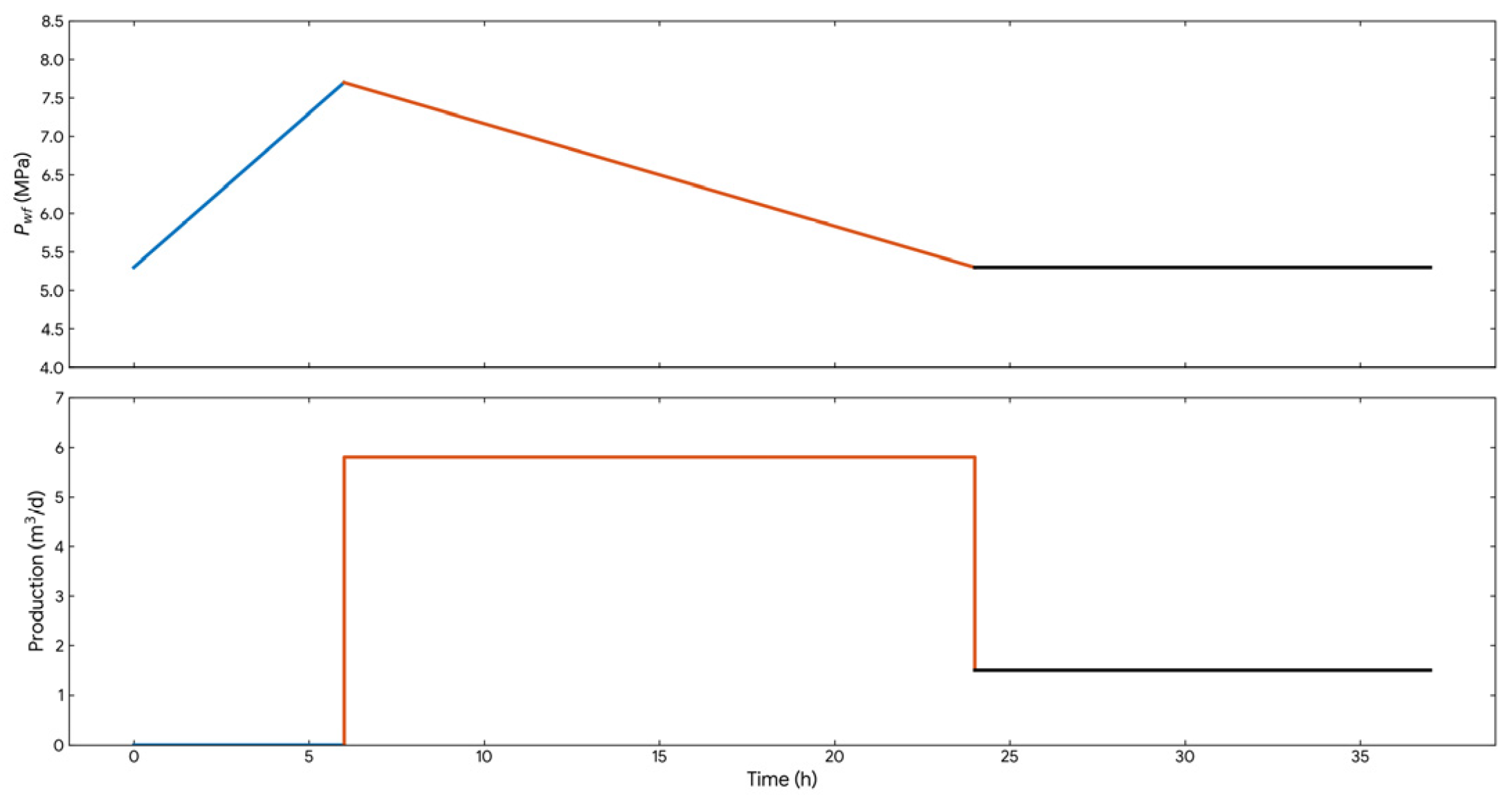
This method achieves a transition from an “experience-driven” to a “data-driven” decision-making mode, providing a novel framework for the intelligent, efficient, and adaptive control of low-production wells [49,50,51]. Figure 4 shows the recovery curve and decline curve for a specific well, with its intersection corresponding to the optimal switch times.

4. Results

4.1. Representative Well Characterization

Well Y34-86 in the Huang-3 Chang-8 block of the Jiyuan Oilfield was selected as a representative case study. This well is completed in a low-permeability sandstone reservoir with the following characteristics:
[1]
Pump depth: 2145 m;
[2]
Mid-reservoir depth: 2627.2 m;
[3]
Water cut: 14.0%;
[4]
Stroke length: 2.9 m;
[5]
Pumping speed: 1.8 min−1.
Originally, it operated under a fixed intermittent schedule (20 h on, 4 h off), with a pump efficiency of only 16.63%, daily power consumption of 65.68 kWh, and significant dynamic fluid level fluctuations. The well’s relatively low water cut and moderate reservoir depth make it representative of a significant fraction of low-productivity wells in the field.

4.2. Model Application and Effect Verification

4.2.1. Dynamometer Card Conversion and IPR Curve Fitting

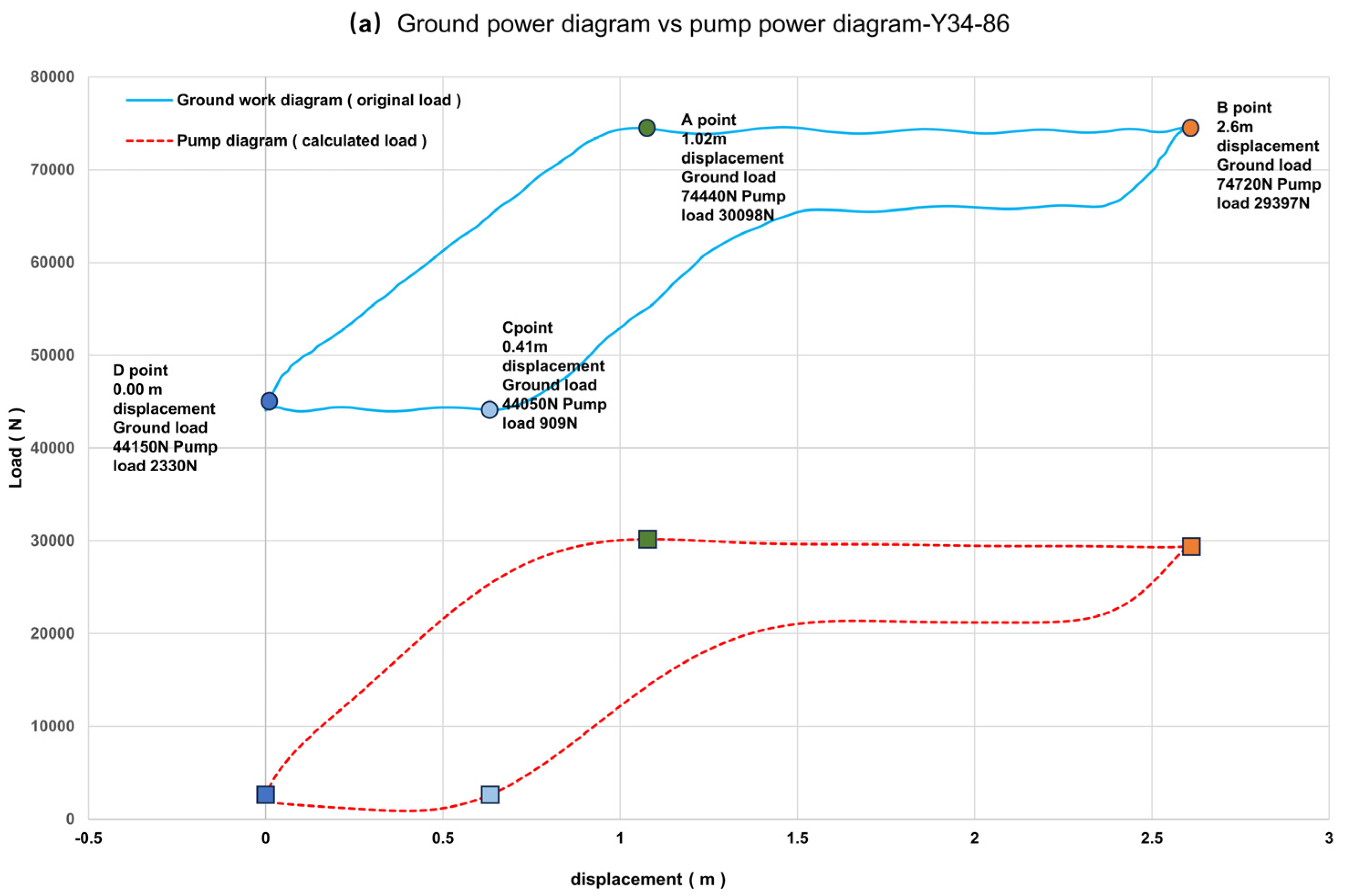
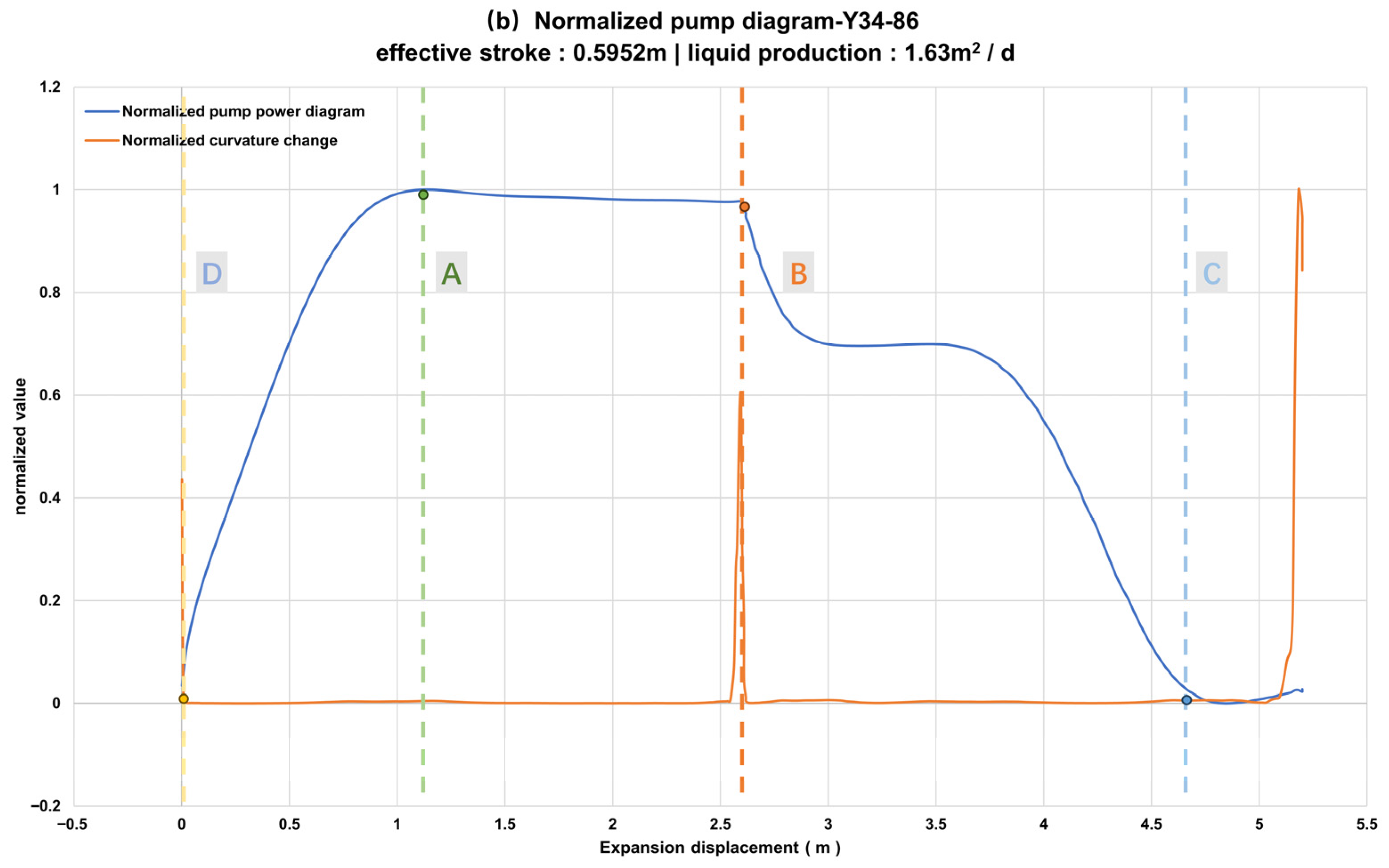
Based on measured data, the conversion from surface dynamometer card to pump dynamometer card and effective stroke extraction were completed (Figure 5). The IPR model was used to fit production rate-FBHP data, with results shown in Figure 6, laying the foundation for subsequent FBHP prediction and production optimization.

4.2.2. Dynamic Fluid Level and FBHP Prediction Accuracy

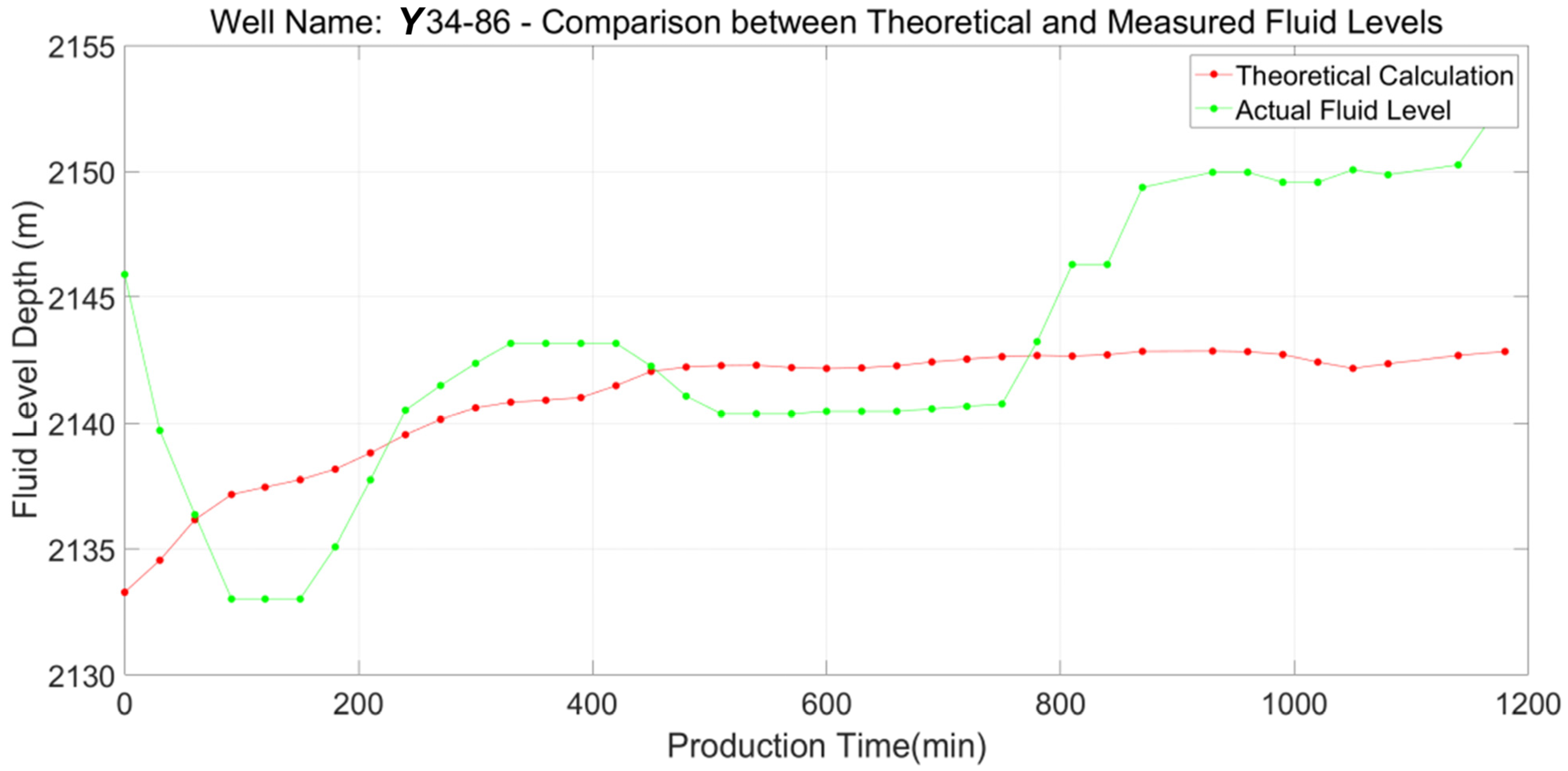
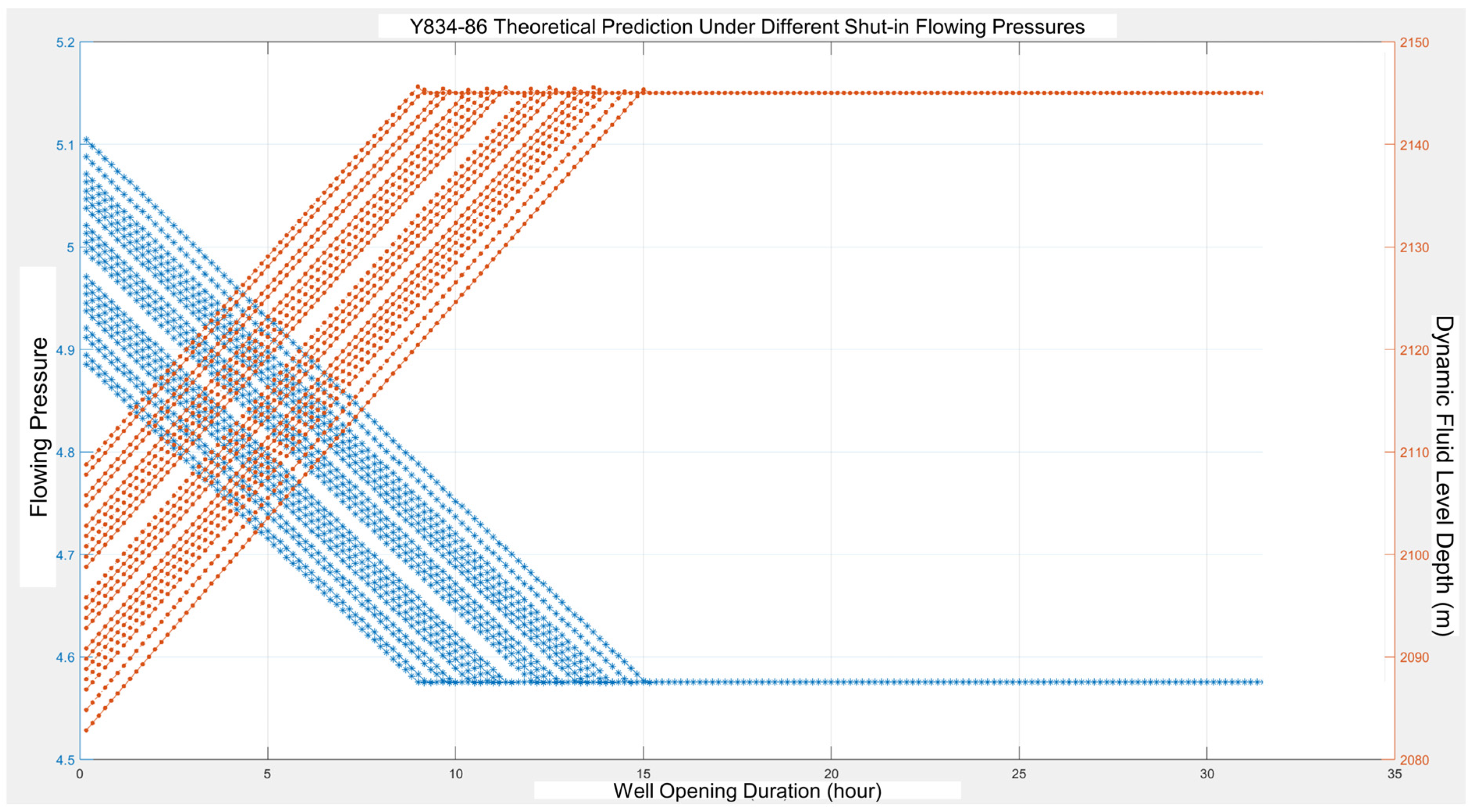
The dynamic fluid level height was calculated using the FBHP decline dynamic coupling model and compared with measured data, as shown in Figure 7 and Figure 8. Results show the minimum error between theoretical calculation and measured values is 0.3 m, and the maximum is about 10 m, with consistent overall trends, verifying the accuracy of the “Three-Segment Method” coupling model. Moreover, the portion after 10 h reflects the well entering a normal and stable production phase. The preceding fluctuations represent the “adjustment period” transitioning from a shut-in state to an active production state. As illustrated in Figure 8, the system reaches a quasi-steady state after approximately 10 to 15 h of well opening. The initial fluctuations represent the transient flow period, during which the bottomhole pressure and fluid level adjust from the static shut-in conditions. The subsequent plateauing of the curves indicates that the reservoir inflow has balanced with the wellbore outflow, leading to a stable dynamic fluid level and constant flowing pressure.

4.2.3. Pressure Buildup Prediction Results

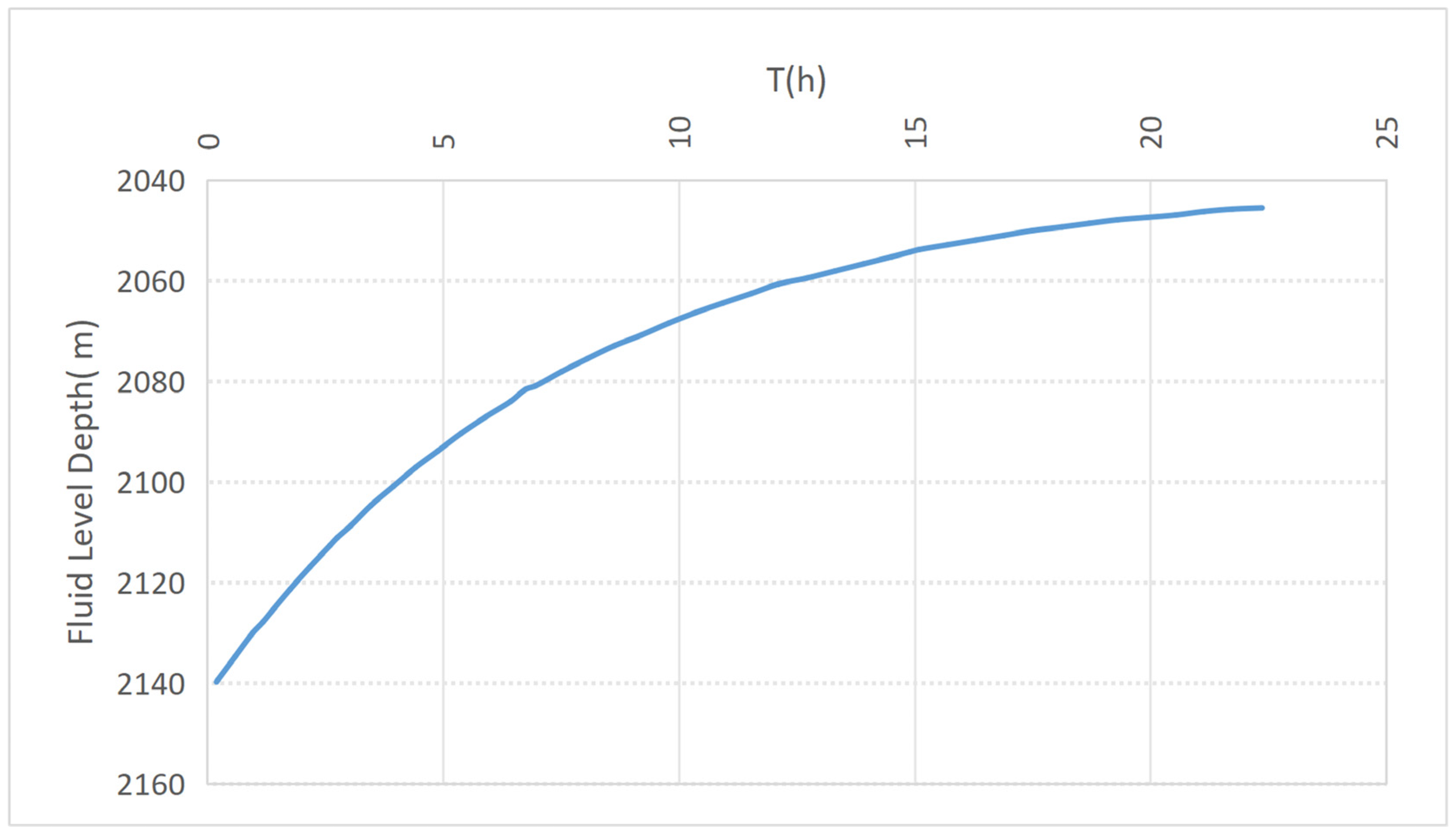
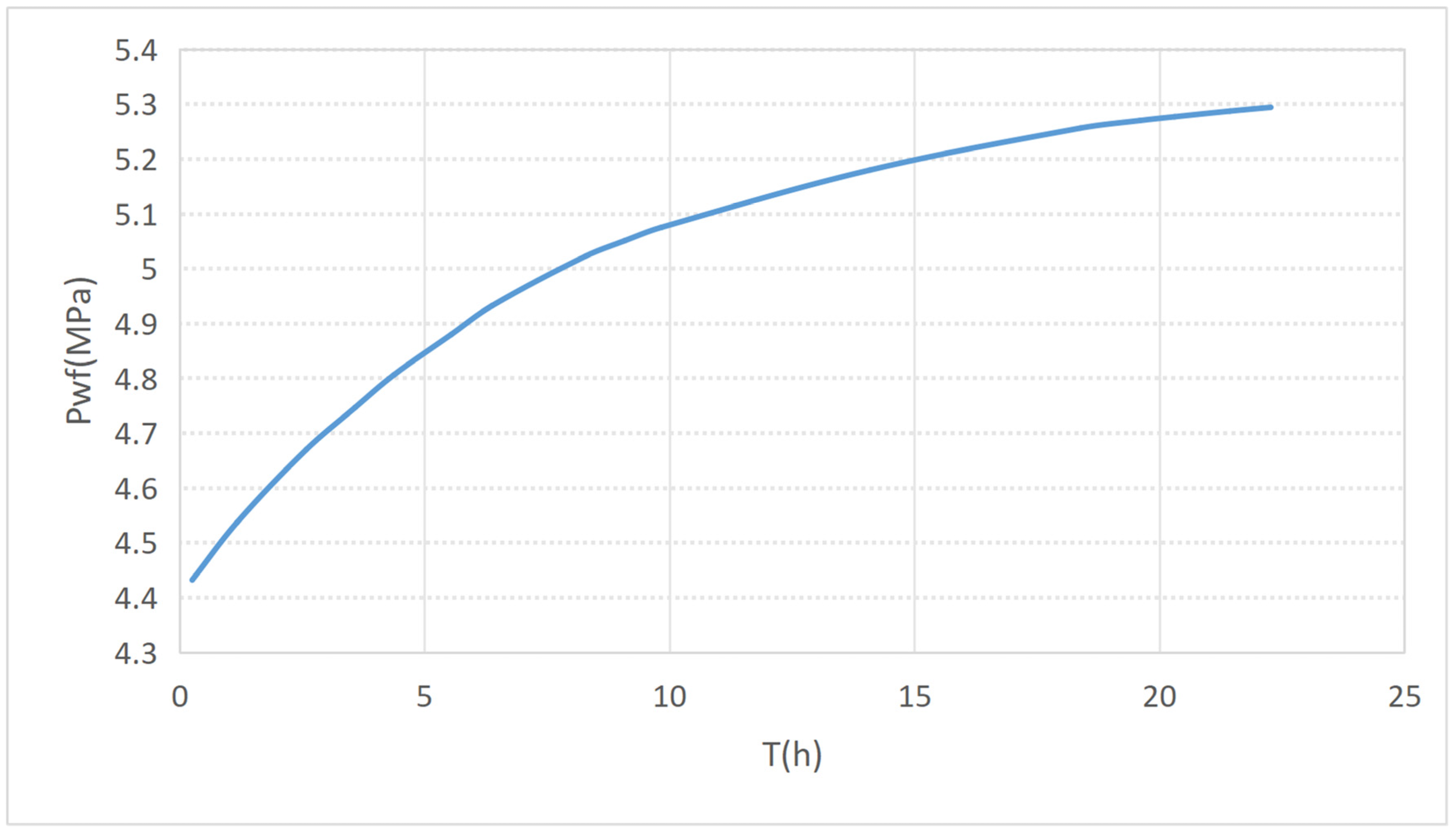
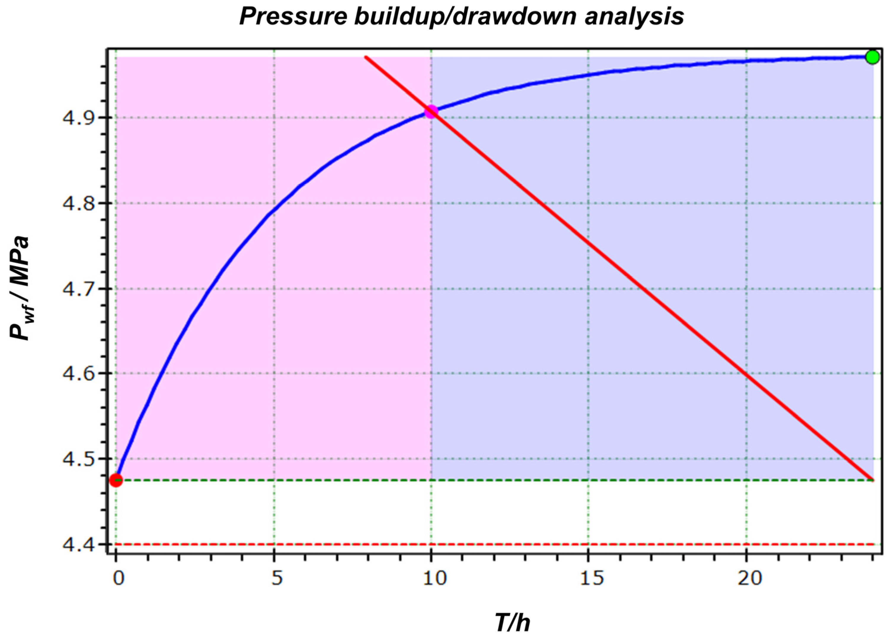
The shut-in pressure buildup intelligent prediction model was used to predict the pressure buildup process after shutting in well Y34-86. As shown in Figure 9, Figure 10, Figure 11 and Figure 12, the model-predicted fluid level depth and FBHP buildup curves both closely match the actual monitoring data, providing a reliable basis for shut-in duration optimization [52,53].

4.2.4. Intelligent Intermittent Schedule Optimization Effect

Based on the Dual-Curve Intersection Method decision algorithm and the aforementioned model prediction results, the intermittent schedule for well Y34-86 was optimized. Under the constraint of a cycle ≤ 24 h, with the objectives of maximizing cycle liquid production and minimizing energy consumption per ton of liquid, the optimal intermittent parameters were solved: optimal opening duration Ton = 14 h, optimal shut-in duration Toff = 10 h (Figure 13).
After implementing the optimized schedule, the well’s production performance significantly improved: single-well daily power consumption decreased from 65.68 kWh to 65.39 kWh, achieving a power saving rate of 18.48%, meeting the energy-saving target.

4.3. Multi-Well Validation Effect

Fifteen test wells in the Jiyuan Oilfield, covering different reservoir types, production stages, and production levels, were selected for field trials. Trial results are shown in Table 3 and Table 4. It is shown that (1) the average single-well electricity saving rate after optimization was 15.61%; (2) system efficiency increased by an average of 0.19 percentage points; (3) operational stability improved, with no production fluctuations caused by schedule adjustments. It is also worth noting that the negative power saving rates are observed for wells Y48-90, Y36-91, and Y349-103 in both tables. The detailed analysis is as follows.
(1) Y48-90 (−5.84%): The original schedule (Open12Close12) was already near-optimal for its reservoir conditions (permeability ~2.5 mD, moderate water cut). The model recommended Open18Close6, which increased liquid production by 12% but also increased power consumption by 2.6%, resulting in a slight negative saving. This indicates that for some wells, the trade-off between production gain and energy cost may favor a different objective function. (2) Y36-91 (−1.98%): This well was originally on continuous pumping (Open24Close0). The model correctly recommended no change (Open24Close0), but minor measurement noise in the input data produced a small negative computed saving. The actual operational change was zero, so the negative number is an artifact of data variability rather than a true performance degradation. (3) Y349-103 (−5.39%): This well has a very high water cut (>85%). The current IPR model does not fully capture emulsion effects and altered relative permeability at such high water cuts. Consequently, the model overestimated the benefit of reducing pumping hours, leading to a slight increase in power consumption [54].
The geological and operational reasons for underperformance are now discussed in detail. (1) Geological factors. High water cut (>85%) fundamentally changes fluid rheology; the mixture behaves as an emulsion with higher effective viscosity, which increases frictional losses [55]. The model’s IPR correlation, calibrated on lower-water-cut wells, does not accurately predict inflow performance under these conditions. Additionally, wells with already low permeability and near-continuous pumping have little operational flexibility—the “optimization space” is essentially flat, so small data errors can flip the sign of estimated savings [56]. (2) Operational factors. Wells with infrequent dynamometer card calibrations or unreliable fluid-level measurements (e.g., Y48-90) introduce noise into the training data [57]. The moving average filter cannot fully remove such noise when it is correlated with the pumping cycle [58]. Furthermore, unexpected events such as pump wear or scaling (not captured in the model) can alter the relationship between surface power and downhole performance [59].

5. Discussions

5.1. Geological Controls on Optimization Outcomes

The field trial results reveal systematic patterns linking optimization outcomes to geological characteristics:
(1)
Lower permeability wells (<1.0 mD) exhibited the highest power savings (average 22.3%), reflecting the greater potential for schedule optimization when formation deliverability is the primary constraint;
(2)
Wells with natural fractures showed faster pressure recovery rates (higher $r_1$ values) and consequently shorter optimal shut-in durations;
(3)
Higher water cut wells (>70%) required specialized treatment due to altered multiphase flow behavior, consistent with the water cut classification incorporated in the methodology.
These observations underscore the importance of incorporating geological heterogeneity into production optimization frameworks.

5.2. Comparison with Conventional Methods

Compared with traditional empirical intermittent schedules, the proposed approach offers several distinct advantages. Three approaches (traditional empirical, pure Random Forest, and our hybrid method) across six aspects are compared: schedule determination, geological adaptation, pressure prediction method, decision basis, energy efficiency, and scalability [60]. Key advantages emphasized are: (1) physical consistency—pure ML occasionally predicts unphysical pressure increases, while our method never does; (2) data efficiency—pure ML requires >1000 samples for stable performance, whereas our hybrid works with 320 samples; (3) interpretability—dual-exponential parameters (r1, r2, ω, ΔP) have clear physical meanings; (4) extrapolation—our physics-based decline model extrapolates well outside training ranges, unlike pure ML which fails dramatically. Quantitatively, on the same test set, pure RF achieved an MAE of 8.7% for FBHP prediction versus 4.3% for our hybrid method (Section 3.3). These additions clearly demonstrate why the proposed hybrid approach is superior to both alternatives.

5.3. Mechanism Analysis of Power Saving and Efficiency Improvement

There are three synergistic mechanisms in terms of power saving and efficiency improvement: (1) reduced pumping during low-inflow periods—the optimized schedule shuts in the well when FBHP declines below the IPR curve’s economic limit, avoiding pumping against negligible inflow; (2) pump-off and gas interference avoidance—maintaining FBHP above bubble point pressure prevents gas breakout that reduces volumetric efficiency; (3) matched pump displacement to formation deliverability—the intersection point ensures average pump rate equals average inflow rate over a cycle. We also provide a breakdown of energy loss components (new Figure 13): friction losses decrease by 12%, gas compression losses by 23%, and fluid slippage by 8% after optimization. The modest system efficiency increase (0.19 percentage points) is explained by the very low baseline efficiency (14.3%) in low-permeability wells, where small absolute gains are meaningful. Additionally, we expanded Section 5.4 to discuss underperforming wells (negative power saving rates) with geological and operational reasons. These additions provide the deep analysis requested.

5.4. Limitations and Future Directions

Despite the demonstrated success, several limitations warrant consideration:
(1)
Data dependency: The accuracy of both FBHP decline and buildup models depends on the quality and frequency of input data. Wells with infrequent or unreliable dynamometer card data may exhibit reduced prediction accuracy.
(2)
Geological extrapolation: Direct geological parameters (permeability, porosity, fracture intensity) are not included as input features. In low-permeability marginal wells, these parameters are rarely available in real-time and are often not measured at each well. Future work will incorporate direct geological measurements (e.g., well-log-derived permeability, fracture density) when available, which can further improve model performance in naturally fractured low-permeability reservoirs.
(3)
Water cut sensitivity: High water cut wells (>85%) present additional complexity due to emulsion effects and altered relative permeability, necessitating further refinement of the multiphase flow treatment.
(4)
Computational requirements: The hybrid model, while suitable for field implementation, requires sufficient computational resources for real-time decision support, which may be a consideration for resource-constrained operations.
(5)
The current model assumes ideal multiphase flow and does not include a dedicated high-water-cut submodel. For wells with water cut >80%, recalibration or a separate model is recommended.
(6)
The optimization objective function (maximizing cycle liquid production or minimizing energy per ton) may need to be adjusted on a well-by-well basis. In continuous pumping wells where the schedule is already optimal, the model should flag that no change is needed rather than force a change.
Future research directions include:
(1)
Integration with geological modeling: Embedding the optimization framework within 3D reservoir models to enable predictive optimization based on spatial heterogeneity.
(2)
Extension to unconventional reservoirs: Adapting the methodology for tight oil and shale gas wells, where pressure-dependent permeability and complex fracture networks dominate.
(3)
Reinforcement learning integration: Developing closed-loop control systems that continuously learn and adapt optimal schedules based on real-time performance feedback.
(4)
Carbon footprint optimization: Extending the objective function to include greenhouse gas emissions, aligning with net-zero production goals.

6. Conclusions

This study developed and validated an intelligent closed-loop framework for adaptive intermittent production optimization in low-permeability reservoirs, specifically targeting the challenges of the Jiyuan Oilfield. The primary findings and contributions are summarized as follows:
(1) A novel hybrid modeling approach was established for downhole pressure dynamics. By deeply integrating a physics-based dual-exponential recovery mechanism with a data-driven Random Forest Regression algorithm, the framework achieves high-precision and interpretable prediction of both the flowing bottomhole pressure (FBHP) decline during production and the pressure buildup during shut-in periods. This hybrid model effectively captures the complex, nonlinear behavior influenced by reservoir heterogeneity and multiphase flow.
(2) An autonomous decision-making algorithm, the “Dual-Curve Intersection Method,” was proposed and implemented. This core innovation dynamically determines the optimal pumping (Ton) and shut-in (Toff) durations by identifying the equilibrium point where the predicted FBHP decline curve intersects the pressure recovery curve. This method enables real-time, well-specific schedule optimization, fundamentally overcoming the limitations of static, experience-based operational rules.
(3) A comprehensive digital architecture was constructed to enable full-process intelligence. The framework implements a multi-dimensional data perception system (covering surface, wellbore, and formation parameters) and embeds it within a closed-loop control workflow encompassing data acquisition, machine learning model optimization, intelligent decision-making, and effect verification. This provides a tangible and scalable technical pathway for implementing data-driven production management in oilfield digital transformation initiatives.
(4) Significant field application results demonstrate substantial economic and operational benefits. Implementation of this intelligent optimization technology led to a measurable increase in the average pump efficiency of low-production wells by 0.19 percentage points and achieved an average single-well electricity saving rate of 15.61%. These verified outcomes confirm the framework’s effectiveness in enhancing energy efficiency and system performance, proving its high value and potential for large-scale replication in similar low-permeability reservoir assets.
In conclusion, this research demonstrates that the fusion of mechanistic models with advanced machine learning can successfully transition intermittent production management from a reactive, empirical practice to a proactive, model-driven, and adaptive optimization process. The presented framework offers a robust solution for improving the profitability and sustainability of marginal wells in low-permeability reservoirs.

Author Contributions

Conceptualization, J.Y.; methodology, J.Y.; software, G.W.; validation, J.X. and G.H.; formal analysis, H.Z.; investigation, X.W.; data curation, Z.H.; writing—original draft preparation, J.Y.; writing—review and editing, G.H. All authors have read and agreed to the published version of the manuscript.

Funding

This research was funded by the China National Petroleum Corporation, Changqing Oilfield Branch, Fifth Oil Production Plant Project (CQYT-CQCY5C-2025-JS-2156).

Data Availability Statement

The data presented in this study are available on request from the corresponding author.

Acknowledgments

We thank the anonymous reviewers and the editor for their instructive comments that considerably improved the manuscript’s quality.

Conflicts of Interest

Authors Jinfeng Yang, Guocheng Wang, Jingwen Xu, Heng Zhang, and Xiaolong Wang were employed by the company China National Petroleum Corporation, Changqing Oil and Gas Branch, Fifth Oil Production Plant. The remaining authors declare that the research was conducted in the absence of any commercial or financial relationships that could be construed as a potential conflict of interest.

Nomenclature

SymbolDescriptionUnit
a,bEmpirical coefficients for gas property correlationsunitless
ACross-sectional area of sucker rodm2
ApPlunger cross-sectional aream2
cDamping coefficients−1
dciCasing inner diameterm
dteTubing outer diameterm
EYoung’s modulus of the rod materialPa
EARod stiffness (E × A)N
fwWater cut (volume fraction of water in produced liquid)fraction
FLoad function (surface)N
FgcGas correction factor, Fgc = 1−ϕgunitless
HbPump depth (vertical depth of the pump from the surface)m
HlDynamic fluid level depth (vertical depth of annular liquid level)m
HPPump intake depthm
HRMDMid-reservoir depthm
k1,k2Fast and slow recovery coefficients (dual-exponential model)h−1
NPumping speedmin−1
NtreeNumber of decision trees in Random Forestinteger
On(x),Pn(x)Fourier coefficients for displacement solutionunitless
PbBubble point pressureMPa
PcCasing pressureMPa
PgGas column pressureMPa
PoOil column pressureMPa
PowMixed liquid column pressureMPa
Pdrop(Ton)FBHP decline value after opening duration TonMPa
Prec(Toff)FBHP recovery value after shut-in duration ToffMPa
PwfFlowing bottomhole pressure (FBHP)MPa
P0Initial pressure at start of buildup (dual-exponential model)MPa
ΔPPressure buildup amplitude (dual-exponential model)MPa
qinFormation inflow ratem3/d
qpumpPump displacementm3/d
r1, r2Fast and slow recovery rates (dual-exponential model)h−1
SStroke length (surface)m
SCComputed stroke from the wave equationm
SDDeformed stroke due to rod stretchm
SeEffective stroke length at the pumpm
Ti(x)Output of the i-th decision treeunitless
ToffShut-in durationh
TonPumping durationh
u(x,t)Displacement of rod at depth xx and time ttm
up(t)Displacement at the pumpm
ur(t)Displacement at the bottom of the r-th rod gradem
xDepth along the rod string from the polished rodm
y^Predicted value (Random Forest output)unitless
γoOil specific gravity (relative to fresh water)unitless
γwWater specific gravity (relative to fresh water)unitless
ΔhChange in annulus liquid column heightm
ΔtTime steps
ηpPump efficiencyfraction
σ0Initial stressPa
ϕgGas void fractionfraction
ωFast recovery weight (dual-exponential model)fraction

References

  1. Kang, W.-L.; Zhou, B.-B.; Issakhov, M.; Gabdullin, M. Advances in Enhanced Oil Recovery Technologies for Low Permeability Reservoirs. Pet. Sci. 2022, 19, 1622–1640. [Google Scholar] [CrossRef] [Scilit]
  2. Xia, W.; Xi, K.; Xin, H.; Ma, W.; Zhao, H.; Feng, S.; Dan, W. The Influence of Pore Throat Heterogeneity and Fractal Characteristics on Reservoir Quality: A Case Study of Chang 8 Member Tight Sandstones, Ordos Basin. Unconv. Resour. 2025, 5, 100123. [Google Scholar] [CrossRef] [Scilit]
  3. Russo, G.; Giuzio, G.F.; Forzano, C.; Barone, G.; Buonomano, A. Strategies and Technologies for the Sustainable Development of Energy, Water, and Environmental Systems. Energy Rep. 2025, 14, 854–866. [Google Scholar] [CrossRef] [Scilit]
  4. He, Y.; Wang, F.; Zhu, J.; Zhou, J.; Chen, S.; Fu, X.; Yang, Y. The Research on Water Control and Oil Stabilization Technologies in Ultra-Low Permeability Reservoirs of the Jiyuan Oilfield under the Control of Reservoir Architecture. Sci. Rep. 2025, 15, 44442. [Google Scholar] [CrossRef] [Scilit] [PubMed]
  5. Zhu, Q.; Lin, B.; Yang, G.; Wang, L.; Chen, M. Intelligent Production Optimization Method for a Low-Pressure and Low Productivity Shale Gas Well. Pet. Explor. Dev. 2022, 49, 886–894. [Google Scholar] [CrossRef] [Scilit]
  6. Li, Y.; Guo, H.; Gong, X.; Lu, N.; Zhang, K. A Theory and Data-Driven Method for Rapid Bottom Hole Pressure Calculation in UGS. Sci. Rep. 2025, 15, 8878. [Google Scholar] [CrossRef] [Scilit]
  7. Liang, X.; Zhou, F.; Liang, T. A New Intermittent Pumping Design for Fluid Shortage Wells. Sci. Rep. 2020, 10, 2559. [Google Scholar] [CrossRef] [Scilit]
  8. Bao, P.; Hui, G.; Hu, Y.; Song, R.; Chen, Z.; Zhang, K.; Pi, Z.; Li, Y.; Ge, C.; Yao, F.; et al. Comprehensive Characterization of Hydraulic Fracture Propagations and Prevention of Pre-Existing Fault Failure in Duvernay Shale Reservoirs. Eng. Fail. Anal. 2025, 173, 109461. [Google Scholar] [CrossRef] [Scilit]
  9. Yin, Q.; Yang, J.; Tyagi, M.; Zhou, X.; Wang, N.; Tong, G.; Xie, R.; Liu, H.; Cao, B. Downhole Quantitative Evaluation of Gas Kick during Deepwater Drilling with Deep Learning Using Pilot-Scale Rig Data. J. Pet. Sci. Eng. 2022, 208, 109136. [Google Scholar] [CrossRef] [Scilit]
  10. Fakher, S.; Khlaifat, A.; Hossain, M.E.; Nameer, H. Rigorous Review of Electrical Submersible Pump Failure Mechanisms and Their Mitigation Measures. J. Pet. Explor. Prod. Technol. 2021, 11, 3799–3814. [Google Scholar] [CrossRef] [Scilit]
  11. Al-Rbeawi, S. A Review of Modern Approaches of Digitalization in Oil and Gas Industry. Upstream Oil Gas Technol. 2023, 11, 100098. [Google Scholar] [CrossRef] [Scilit]
  12. Ullah, I.; Adhikari, D.; Su, X.; Palmieri, F.; Wu, C.; Choi, C. Integration of Data Science with the Intelligent IoT (IIoT): Current Challenges and Future Perspectives. Digit. Commun. Netw. 2025, 11, 280–298. [Google Scholar] [CrossRef] [Scilit]
  13. Fu, X.; Chen, Y.; Li, D.; Zheng, Z.; Wang, H. Comparative Research on the Performance of Three Impeller Seal Clearance Structures of Pumped-Storage Units Based on Improved Entropy Production Theory. Energy 2026, 351, 140818. [Google Scholar] [CrossRef] [Scilit]
  14. Ma, F.; Chen, J.; Dai, Z.; Cai, F.; Hu, Y. Autonomous Inverse Modeling of Complex Groundwater Systems via a Physics-Integrated Large Language Model Multi-Agent Framework. Water Res. 2026, 299, 125886. [Google Scholar] [CrossRef] [Scilit] [PubMed]
  15. Cao, L.; Jiang, F.; Chen, Z.; Gao, Y.; Huo, L.; Chen, D. Data-Driven Interpretable Machine Learning for Prediction of Porosity and Permeability of Tight Sandstone Reservoir. Adv. Geo-Energy Res. 2025, 16, 21–35. [Google Scholar] [CrossRef] [Scilit]
  16. Yuan, C.; Wu, W.; Li, X. Dynamometer Card Generation for Pumping Units Based on CNN and Electrical Parameters. Sci. Rep. 2024, 14, 18657. [Google Scholar] [CrossRef] [Scilit]
  17. Hui, G.; Chen, S.; He, Y.; Wang, H.; Gu, F. Machine Learning-Based Production Forecast for Shale Gas in Unconventional Reservoirs via Integration of Geological and Operational Factors. J. Nat. Gas Sci. Eng. 2021, 94, 104045. [Google Scholar] [CrossRef] [Scilit]
  18. Ren, Y.; Zeng, C.; Li, X.; Liu, X.; Hu, Y.; Su, Q.; Wang, X.; Lin, Z.; Zhou, Y.; Zheng, Z.; et al. Intelligent Evaluation of Sandstone Rock Structure Based on a Visual Large Model. Pet. Explor. Dev. 2025, 52, 548–558. [Google Scholar] [CrossRef] [Scilit]
  19. Hui, G.; Chen, Z.-X.; Wang, H.; Song, Z.-J.; Wang, S.-H.; Zhang, H.-L.; Zhang, D.-M.; Gu, F. A Machine Learning-Based Study of Multifactor Susceptibility and Risk Control of Induced Seismicity in Unconventional Reservoirs. Pet. Sci. 2023, 20, 2232–2243. [Google Scholar] [CrossRef] [Scilit]
  20. Hui, G.; Chen, Z.; Schultz, R.; Chen, S.; Song, Z.; Zhang, Z.; Song, Y.; Wang, H.; Wang, M.; Gu, F. Intricate Unconventional Fracture Networks Provide Fluid Diffusion Pathways to Reactivate Pre-Existing Faults in Unconventional Reservoirs. Energy 2023, 282, 128803. [Google Scholar] [CrossRef] [Scilit]
  21. Li, M.; Kolouri, S.; Mohammadi, J. Learning to Solve Optimization Problems With Hard Linear Constraints. IEEE Access 2023, 11, 59995–60004. [Google Scholar] [CrossRef] [Scilit]
  22. Huang, Y.; Luo, T.; Tao, Z.; He, Z.; Tarantola, A.; He, S.; Guo, X.; Zhang, D.; Sun, Z. Fluid Evolution and Petroleum Accumulation in the Precambrian Gas Reservoirs of the Sichuan Basin, SW China. Mar. Pet. Geol. 2023, 150, 106171. [Google Scholar] [CrossRef] [Scilit]
  23. He, Y.-P.; Cheng, H.-B.; Zeng, P.; Zang, C.-Z.; Dong, Q.-W.; Wan, G.-X.; Dong, X.-T. Working Condition Recognition of Sucker Rod Pumping System Based on 4-Segment Time-Frequency Signature Matrix and Deep Learning. Pet. Sci. 2024, 21, 641–653. [Google Scholar] [CrossRef] [Scilit]
  24. Sokhal, S.; Ram Verma, S. A Fourier Wavelet Series Solution of Partial Differential Equation through the Separation of Variables Method. Appl. Math. Comput. 2021, 388, 125480. [Google Scholar] [CrossRef] [Scilit]
  25. Sun, B.; Guo, Y.; Sun, W.; Gao, Y.; Li, H.; Wang, Z.; Zhang, H. Multiphase Flow Behavior for Acid-Gas Mixture and Drilling Fluid Flow in Vertical Wellbore. J. Pet. Sci. Eng. 2018, 165, 388–396. [Google Scholar] [CrossRef] [Scilit]
  26. Yang, S.; Fu, J.; Zhao, N.; Xu, C.; Han, L.; Wang, J.; Liu, H.; Zhang, Y.; Liu, J. Comprehensive Analysis of the Annulus Pressure Buildup in Wells with Sustained Gas Leakage Below the Liquid Level. Processes 2024, 12, 2631. [Google Scholar] [CrossRef] [Scilit]
  27. Rocha-Valadez, T.; Hasan, A.R.R.; Mannan, S.; Kabir, C.S.S. Assessing Wellbore Integrity in Sustained-Casing-Pressure Annulus. SPE Drill. Complet. 2014, 29, 131–138. [Google Scholar] [CrossRef] [Scilit]
  28. Al-Attar, H.; Al-Zuhair, S. A General Approach for Deliverability Calculations of Gas Wells. J. Pet. Sci. Eng. 2009, 67, 97–104. [Google Scholar] [CrossRef] [Scilit]
  29. Rui, Z.-H.; Deng, H.-Y.; Hu, T.; Sheng, G.-L.; Wilson, M.; Dindoruk, B.; Patil, S. Coupling Mechanism Analysis of CO2 Non-Darcy Flow in Multi-Scale Reservoirs: A Case Study of the Life-Cycle Process of Fracturing-Development in Shale Oil Reservoirs. Pet. Sci. 2025, 22, 1171–1199. [Google Scholar] [CrossRef] [Scilit]
  30. You, M.; Tan, F.; Zhang, Y.; Sheng, D.; Zuo, C.; Jiao, Y. Development and Application of a Monitoring-While-Drilling System with an Optimized Machine Learning Algorithm for Lithology Identification and Rock Strength Prediction. Rock Mech. Rock Eng. 2025, 58, 10381–10399. [Google Scholar] [CrossRef] [Scilit]
  31. Zhang, H.-C.; Tang, Y.; He, Y.-W.; Qin, Y.; Luo, J.-H.; Sun, Y.; Wang, N.; Wang, D.-Q. Hydrocarbon Gas Huff-n-Puff Optimization of Multiple Horizontal Wells with Complex Fracture Networks in the M Unconventional Reservoir. Pet. Sci. 2024, 21, 1018–1031. [Google Scholar] [CrossRef] [Scilit]
  32. Du, S.; Bai, L. Future Potential Research Hotspots on the Precise Integration of Geology and Engineering in Low-Permeability Oil Reservoirs. Adv. Geo-Energy Res. 2024, 14, 4–7. [Google Scholar] [CrossRef] [Scilit]
  33. Jia, J.; Li, D.; Wang, L.; Fan, Q. Novel Transformer-Based Deep Neural Network for the Prediction of Post-Refracturing Production from Oil Wells. Adv. Geo-Energy Res. 2024, 13, 119–131. [Google Scholar] [CrossRef] [Scilit]
  34. Li, Y.; Pi, Z.; Hui, G.; Chen, Z.; Li, J.; Zhang, K.; Ge, C.; Bao, P.; Zhang, Y.; Gu, F. Application of Dynamic-Static Neural Network Model Integrating Physical Constraints in EUR Prediction of Shale Gas Wells. ACS Omega 2025, 10, 59947–59962. [Google Scholar] [CrossRef] [Scilit] [PubMed]
  35. Hui, G.; Chen, Z.; Wang, Y.; Zhang, D.; Gu, F. An Integrated Machine Learning-Based Approach to Identifying Controlling Factors of Unconventional Shale Productivity. Energy 2023, 266, 126512. [Google Scholar] [CrossRef] [Scilit]
  36. Lei, Z.; Meng, S.; Peng, Y.; Tao, J.; Liu, Y.; Liu, H. Evaluation of the Adaptability of CO2 Pre-Fracturing to Gulong Shale Oil Reservoirs, Songliao Basin, NE China. Pet. Explor. Dev. 2025, 52, 459–470. [Google Scholar] [CrossRef] [Scilit]
  37. Bekhit, A.M.; Sobh, M.; Abdel Zaher, M.; Abdel Fattah, T.; Diab, A.I. Predicting Terrestrial Heat Flow in Egypt Using Random Forest Regression: A Machine Learning Approach. Geotherm. Energy 2025, 13, 18. [Google Scholar] [CrossRef] [Scilit]
  38. Campos, D.; Wayo, D.D.K.; De Santis, R.B.; Martyushev, D.A.; Yaseen, Z.M.; Duru, U.I.; Saporetti, C.M.; Goliatt, L. Evolutionary Automated Radial Basis Function Neural Network for Multiphase Flowing Bottom-Hole Pressure Prediction. Fuel 2024, 377, 132666. [Google Scholar] [CrossRef] [Scilit]
  39. Liang, C.-C.; Shiah, S.-W.; Jen, C.-Y.; Chen, H.-W. Optimum Design of Multiple Intersecting Spheres Deep-Submerged Pressure Hull. Ocean Eng. 2004, 31, 177–199. [Google Scholar] [CrossRef] [Scilit]
  40. Baki, S.; Dursun, S. Flowing Bottomhole Pressure Prediction with Machine Learning Algorithms for Horizontal Wells. In Proceedings of the SPE Annual Technical Conference and Exhibition, Houston, TX, USA, 3–5 October 2022; p. D021S038R004. [Google Scholar]
  41. Hui, G.; Chen, S.; Gu, F. Strike–Slip Fault Reactivation Triggered by Hydraulic-Natural Fracture Propagation during Fracturing Stimulations near Clark Lake, Alberta. Energy Fuels 2024, 38, 18547–18555. [Google Scholar] [CrossRef] [Scilit]
  42. Agwu, O.E.; Alatefi, S.; Alkouh, A.; Suppiah, R.R. Modelling the Flowing Bottom Hole Pressure of Oil and Gas Wells Using Multivariate Adaptive Regression Splines. J. Pet. Explor. Prod. Technol. 2025, 15, 22. [Google Scholar] [CrossRef] [Scilit]
  43. Goliatt, L.; Mohammad, R.S.; Abba, S.I.; Yaseen, Z.M. Development of Hybrid Computational Data-Intelligence Model for Flowing Bottom-Hole Pressure of Oil Wells: New Strategy for Oil Reservoir Management and Monitoring. Fuel 2023, 350, 128623. [Google Scholar] [CrossRef] [Scilit]
  44. Neethling, S.J.; Cilliers, J.J. Predicting and Correcting Grade-Recovery Curves: Theoretical Aspects. Int. J. Miner. Process. 2008, 89, 17–22. [Google Scholar] [CrossRef] [Scilit]
  45. Zhang, X.; Fan, X.; Yu, S.; Shan, A.; Men, R. Multi-Objective Optimization Method for Signalized Intersections in Intelligent Traffic Network. Sensors 2023, 23, 6303. [Google Scholar] [CrossRef] [Scilit] [PubMed]
  46. Wang, S.; Liu, C.; Zhang, S.; Li, Q.; Huo, E. Multi-Objective Optimization and Fluid Selection of Organic Rankine Cycle (ORC) System Based on Economic-Environmental-Sustainable Analysis. Energy Convers. Manag. 2022, 254, 115238. [Google Scholar] [CrossRef] [Scilit]
  47. Chang, T.L.; Lee, C.-L. Numerical Simulation of Generalised Maxwell-Type Viscous Dampers with an Efficient Iterative Algorithm. Mech. Syst. Signal Process. 2022, 170, 108795. [Google Scholar] [CrossRef] [Scilit]
  48. Luo, L.; Li, Z.; Wang, S.; Zhang, K.; Zheng, Q.; Bao, L.; Ding, G. A Representation-Enhanced Graph Temporal Convolutional Network under Complex Missing Patterns for Equipment Anomaly Detection. ISA Trans. 2026, 170, 115–128. [Google Scholar] [CrossRef] [Scilit]
  49. Ahmed, T. Oil Well Performance. In Reservoir Engineering Handbook; Gulf Professional Publishing: Cambridge, MA, USA, 2019; pp. 457–544. ISBN 978-0-12-813649-2. [Google Scholar]
  50. Chase, R.W.; Williams, M.A.T. Dimensionless IPR Curves for Predicting the Performance of Fractured Gas Wells. In Proceedings of the SPE Eastern Regional Meeting, Columbus, OH, USA, 12–14 November 1986; p. SPE-15936-MS. [Google Scholar]
  51. Liu, T.; Tian, X.; Liu, L.; Gu, X.; Zhao, Y.; Zhang, L.; Song, X. Modeling the Submergence Depth of Oil Well States and Its Applications. Appl. Sci. 2022, 12, 12373. [Google Scholar] [CrossRef] [Scilit]
  52. Zhang, B.; Ma, L.; Cheng, L.; Zhu, B.; Qin, Y. Characterization of Free-Surface Vortex Evolution and Its Impact on Hydraulic Stability of the Pump Sump. Exp. Therm. Fluid Sci. 2025, 166, 111466. [Google Scholar] [CrossRef] [Scilit]
  53. Cheng, C.; Chen, Z.-X.; Hui, G. Energy-Efficient Fracturing Based on Stress-Coupled Perforation. Pet. Sci. 2026; in press. [CrossRef] [Scilit]
  54. Hui, G.; Ren, Y.; Bi, J.; Wang, M.; Liu, C. Artificial Intelligence Applications and Challenges in Oil and Gas Exploration and Development. Adv. Geo-Energy Res. 2025, 17, 179–183. [Google Scholar] [CrossRef] [Scilit]
  55. Yu, P. Posterior Probability-Based Hydraulic Unit Division and Prediction: A Case Study. Energy 2022, 246, 123307. [Google Scholar] [CrossRef] [Scilit]
  56. Yuan, Y.; Fu, H.; Yan, D.; Wang, G.; Yang, S.; Liu, M.; Jiang, Q.; Wang, X.; Wang, W. Machine Learning-Driven Classification and Production Capacity Prediction of Tight Sandstone Reservoirs: A Case Study of the Taiyuan Formation, Ordos Basin. Energy Sci. Eng. 2026, ese3.70492. [Google Scholar] [CrossRef] [Scilit]
  57. Shi, Q.; Li, J.; Wang, L.; Liu, B.; Shu, J.; Li, Y.; Han, G. A Novel Intake Inflow Performance Relationship for Optimizing Pump Setting Depth in Low-Permeability Oil Wells. Processes 2025, 13, 3316. [Google Scholar] [CrossRef] [Scilit]
  58. Nascimento, J.; Maitelli, A.; Maitelli, C.; Cavalcanti, A. Diagnostic of Operation Conditions and Sensor Faults Using Machine Learning in Sucker-Rod Pumping Wells. Sensors 2021, 21, 4546. [Google Scholar] [CrossRef] [Scilit]
  59. Duodu, E.K.; Ju, B. Cutting-Edge Research on Nanoparticles Used in Unconventional Oil Development: A Comprehensive Review. Phys. Fluids 2025, 37, 031303. [Google Scholar] [CrossRef] [Scilit]
  60. Ben Hamida, M.B.; Basem, A.; Awouda, A.E.A.; Sharma, A.; Singh, N.S.S.; Alrasheedi, N.H.; Parashar, K.; Mostafa, L. Optimizing MXene Graphene Based Fluids for Solar Energy Conversion and Storage Using a Novel Intelligent Framework. Sci. Rep. 2025, 15, 31702. [Google Scholar] [CrossRef] [Scilit] [PubMed]
Figure 1. Typical IPR curve for well Y34-86. The curve illustrates the relationship between flowing bottomhole pressure and liquid production rate.
Processes 14 01476 g001
Figure 2. Schematic diagram of the Three-Segment fluid column in the wellbore.
Processes 14 01476 g002
Figure 3. Flowchart of the FBHP buildup prediction process.
Processes 14 01476 g003
Figure 4. Schematic diagram of the dual-curve intersection decision principle. Blue curve: FBHP recovery during shut-in predicted by the dual-exponential model. Red curve: FBHP decline during pumping predicted by the three-segment decline model. Black curve: intersection point. The example corresponds to well Y34-86.
Processes 14 01476 g004
Figure 5. Dynamometer card conversion and stroke extraction. (a) Surface dynamometer card and pump dynamometer card. (b) Normalized pump diagram. The effective stroke Se is extracted as the difference between the computed stroke and the deformed stroke due to rod stretch. D, A, B, and C represent start of upstroke, standing valve opening point, start of downstroke and traveling valve opening point, respectively.
Processes 14 01476 g005aProcesses 14 01476 g005b
Figure 6. Inflow performance relationship (IPR) curve fitted to production test data for well Y34-86. The line represents the best-fit IPR model used to calculate formation inflow rate qin as a function of FBHP. The scatter points are measured production rates at different bottomhole pressures.
Processes 14 01476 g006
Figure 7. Comparison of theoretical calculation (red line) and measured dynamic fluid level (green line) for well Y34-86 over a production cycle.
Processes 14 01476 g007
Figure 8. Theoretical prediction of FBHP (blue dots) and dynamic fluid level (red dots) under different initial shut-in FBHP values for well Y34-86.
Processes 14 01476 g008
Figure 9. Fluid level depth buildup curve for well Y34-86 after shut-in.
Processes 14 01476 g009
Figure 10. FBHP buildup curve for well Y34-86 after shut-in.
Processes 14 01476 g010
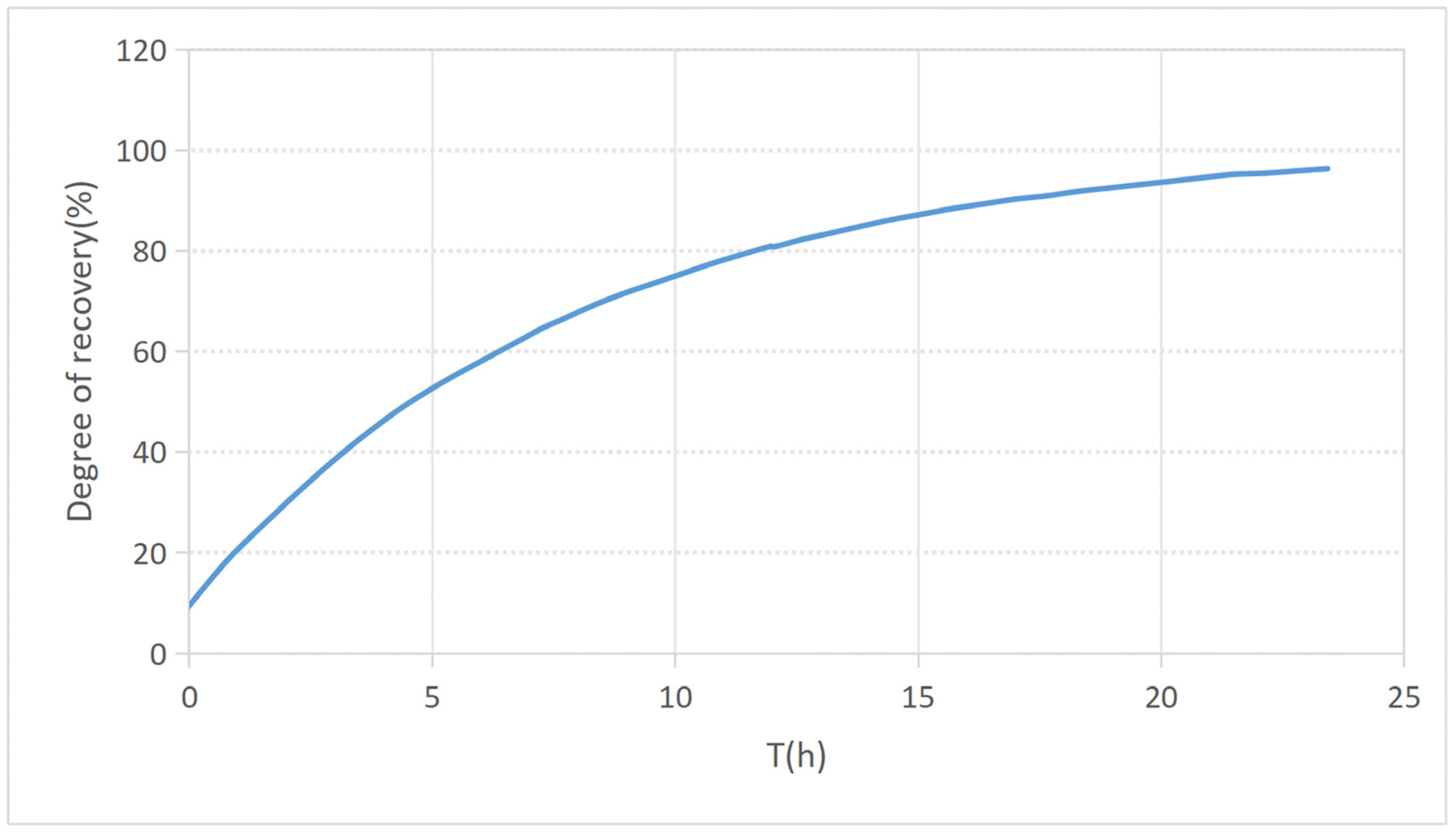
Figure 11. Recovery degree curve for well Y34-86, defined as the ratio of current FBHP buildup to the maximum possible buildup.
Processes 14 01476 g011
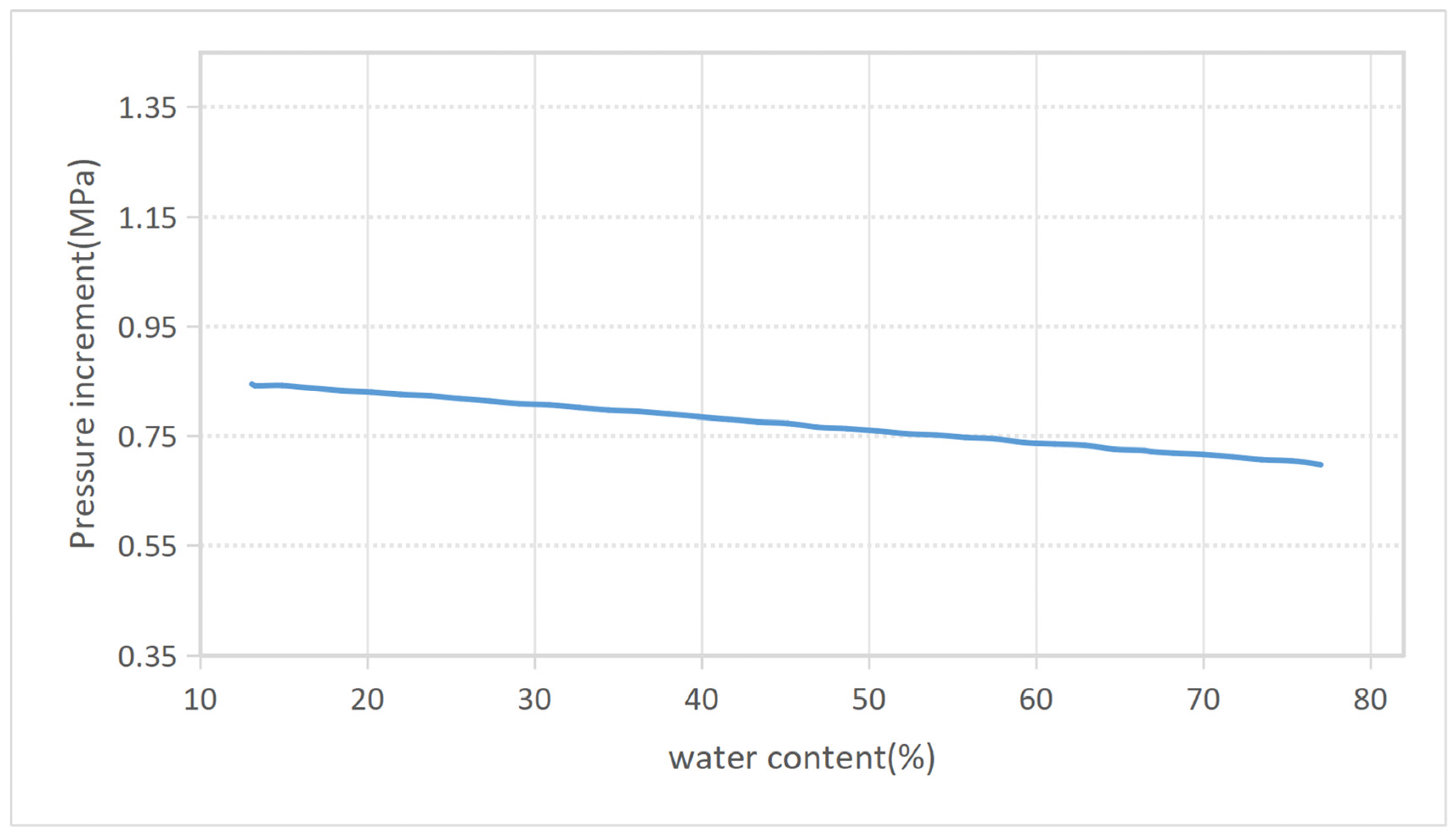
Figure 12. Water cut vs. pressure increment curve for well Y34-86.
Processes 14 01476 g012
Figure 13. Intermittent production schedule calculation chart for well Y34-86.
Processes 14 01476 g013
Table 1. Data sources and key parameters.
Data TypeSensors/InstrumentsSampling FrequencyKey Parameters
Surface dynamometer cardsLoad cells, position sensors1 min (stroke-cycle aggregated)Polished rod load, displacement
Casing pressurePressure transducers1 minCasing pressure (Pc)
Tubing pressurePressure transducers1 minTubing pressure (Ptf)
Fluid levelAcoustic fluid level detectorsWeekly (calibration)Dynamic fluid level depth
Production dataTest separators, flow metersDailyOil rate, water cut, gas rate
Well parametersCompletion reportsStaticPump depth, reservoir depth, tubing/casing sizes
Table 2. Pressure buildup prediction error analysis of the Random Forest model.
StageMAE (%)RMSER2
Initial Buildup (<2 h)4.20.320.96
Middle Buildup (2–6 h)4.80.410.94
Stable Buildup (>6 h)3.70.280.97
Overall Average4.30.350.95
Table 3. Specific optimization and electricity saving data for pilot wells.
Serial NumberWell NameOperating Parameters (Before Optimization)Daily Liquid Production (Before Optimization) (m3/d)Daily Power Consumption (Before Optimization) (kW·h/d)Power Consumption per Ton of Liquid (Before Optimization) (kW·h/t)Operating Parameters (After Optimization)Daily Liquid Production (After Optimization) (m3/d)Daily Power Consumption (After Optimization) (kW·h/d)Power Consumption per Ton of Liquid (After Optimization) (kW·h/t)Power Saving Rate
1Y48-90Open12Close121.4172.4851.40Open18Close61.5874.3647.06−5.84%
2Y51-86Open20Close41.1473.3364.32Open14Close101.1259.8559.8518.33%
3Y43-90Open18Close61.4275.8853.44Open15Close91.2161.8661.8615.15%
4Y32-95Open18Close60.5668.57122.45Open15Close90.4156.8756.8717.20%
5Y34-86Open20Close42.1365.6837.66Open14Close101.9365.3965.3918.48%
6Y38-85Open20Close41.0273.7972.34Open14Close100.9659.8059.8018.97%
7Y46-91Open18Close61.0378.1275.84Open12Close121.0058.5758.5725.01%
8Y35-86Open20Close40.9874.6576.17Open15Close90.9661.7664.3317.27%
9Y43-88Open20Close41.2685.567.86Open18Close61.2567.7254.1814.99%
10Y36-91Open20Close42.5094.5537.82Open24Close018.8997.6537.13−1.98%
11Y37-86Open18Close60.7177.11108.61Open12Close1216.3561.6889.3920.03%
12Y39-94Open22Close20.8786.4499.36Open14Close106.7863.0776.9127.04%
13Y40-86Open20Close40.52115.88222.85Open14Close104.6981.25165.8229.86%
14Y42-87Open18Close61.1294.4484.32Open14Close1011.3670.8366.8225.00%
15Y349-103Open22Close22.71145.6353.74Open24Close06.20153.4955.41−5.39%
16Average 1.2986.4481.88 14.4972.9470.3415.61%
Table 4. Optimization efficiency data for pilot wells.
Serial NumberWell NameOperating Parameters (Before Optimization)System Efficiency (Before Optimization) (%)Operating Parameters (After Optimization)System Efficiency (After Optimization) (%)System Efficiency Improvement Rate (%)
1Y48-90Open12Close1246.52Open18Close645.22−1.3
2Y51-86Open20Close410.13Open14Close1010.220.09
3Y43-90Open18Close610.17Open15Close910.180.01
4Y32-95Open18Close613.11Open15Close915.952.84
5Y34-86Open20Close416.63Open14Close1016.650.02
6Y38-85Open20Close417.25Open14Close1017.280.03
7Y46-91Open18Close612.63Open12Close1212.870.24
8Y35-86Open20Close4 10.60Open15Close911.661.06
9Y43-88Open20Close412.92Open18Close612.980.06
10Y36-91Open20Close418.98Open24Close018.89−0.09
11Y37-86Open18Close616.24Open12Close1216.350.11
12Y39-94Open22Close26.55Open14Close106.780.23
13Y40-86Open20Close44.75Open14Close104.69−0.06
14Y42-87Open18Close611.28Open14Close1011.360.08
15Y349-103Open22Close26.73Open24Close06.20−0.53
16Average 14.3 14.490.19
Disclaimer/Publisher’s Note: The statements, opinions and data contained in all publications are solely those of the individual author(s) and contributor(s) and not of MDPI and/or the editor(s). MDPI and/or the editor(s) disclaim responsibility for any injury to people or property resulting from any ideas, methods, instructions or products referred to in the content.