Hydrogen Production from Agro-Industrial Residues of the Wine Industry: A Techno-Economic Analysis

Abstract

The growing global energy demand and the urgent need to decarbonize the energy sector are driving the search for renewable and low-impact energy sources. Within this context, the conversion of biomass into hydrogen represents a viable pathway to sustainable energy, enabling both carbon mitigation and circular use of agricultural residues. This research focuses on the simulation of an integrated system that converts viticulture residues, vine prunings and grape stalks into biogenic hydrogen through a combination of pretreatment, gasification, and upgrading stages. The analysis of four different supply scenarios shows that the integration of prunings and stalks ensures the highest hydrogen yield (6.61 × 10⁵ Nm³/year of H₂) and the highest energy self-sufficiency, with 25% of produced syngas used to partially cover internal energy demand. Gasification enables the process to be carbon-negative, saving 1.18 kgCO₂eq for Nm³ of H₂ produced, and economically competitive, with a break-even price of 3.81 €/kg and a return on investment of ten years. The study aligns with the decarbonization goals of the European energy transition, promoting local and circular valorization of agro-industrial waste.

1. Introduction

In the global energy landscape, the continuous growth in energy demand and the urgent need to mitigate greenhouse gas emissions have focused significant attention over recent decades on the development of renewable energy solutions. Despite this trend, fossil fuels still account for most of global energy consumption and remain the primary drivers of carbon dioxide emissions. Consequently, energy transition strategies are increasingly promoting the adoption of solutions capable of integrating security of supply, reduced environmental impact, and the efficient use of available resources [1].

Biomass, particularly that of agricultural and forestry origin, represents a locally available renewable resource that can concretely contribute to the reduction of net CO₂ emissions [2].

In the viticulture sector, one of the most significant agro-industrial compartments in Europe, in which Italy plays a prominent role (approximately 20% of the European vineyard area is Italian [3]), large quantities of residues are generated annually, such as pruning canes (sarments), grape stalks, grape pomace, and marc. Often, the valorization of waste from such processes entails high costs and environmental impacts, undermining the very concept of value recovery. For instance, pruning sarments, composed of residual wood from the vineyard pruning process, are traditionally managed in two alternative ways: through mulching and direct return to the vineyards, allowing nutrient recycling but potentially contributing to the spread of pathogens and pests, or through open-field burning, which releases pollutants into the atmosphere, degrading air quality [4].

An alternative to these options is the energy recovery of these biomass residues. Pruning canes and stalks, if properly collected and pretreated, can serve as feedstock for gasification processes.

Specifically, this article examines the biomass waste obtained from six winery facilities and the vineyards of a single winery (Carpi) of the Cantine Riunite & CIV group for the validation of the developed simulation models.

Biomass gasification appears to be the optimal pathway for treating lignocellulosic biomass. It consists of a set of thermochemical reactions in which biomass is converted into a combustible gaseous mixture (syngas, primarily composed of hydrogen, carbon monoxide, and methane), tars, and solid carbonaceous products (biochar). In the present study, a fixed-bed downdraft gasifier was selected as the most appropriate reactor configuration for the intended application. In this type of reactor, four main zones can be identified along the reactor axis: a drying zone in the upper section, followed by pyrolysis, combustion, and reduction zones. Owing to the complexity of the underlying physical and chemical phenomena, the definition of operating conditions and process parameters is of crucial importance. It should be noted that each type of biomass, possessing distinct physical, mechanical and chemical characteristics, requires highly diversified gasification processes; simultaneously, the gasification products are highly variable based on the specific boundary conditions, such as reactor pressure and gasifying-agent composition [5].

Hydrogen produced through gasification and subsequent syngas upgrading represents a strategic energy carrier within the European decarbonization framework [6]. It can be utilized in stationery and mobility applications, contributing to emission reductions in hard-to-abate sectors [6]. The production of biogenic hydrogen (i.e., hydrogen produced from residual biomass) offers the advantage of reconciling energy needs with the waste management requirements [7,8].

This work fits into this scenario by proposing the simulation of an integrated system for the conversion of viticultural residues into biogenic hydrogen. The system, described in detail in Fantasia et al. [9], encompasses phases of biomass pretreatment, gasification, and subsequent upgrading of the produced gas. In this work, the system is applied to four different supply scenarios, distinguished by the type of biomass utilized:

• Scenario A: Valorization of vineyard pruning canes produced annually by the vineyards related to the Carpi winery of the Riunite & CIV group.
• Scenario B: Valorization of grape stalks produced annually by the Carpi winery of the Riunite & CIV group.
• Scenario C (A + B): Valorization of both pruning canes and grape stalks produced annually by the Carpi winery of the Riunite & CIV group.
• Scenario D: Valorization of grape stalks produced annually by the six wineries of the Riunite & CIV group.

This study, therefore, aims to validate a simulation system for the gasification of viticultural by-products and to compare the four scenarios, analyzing their feasibility from both environmental and economic perspectives.

2. Materials and Methods

The complete considered conversion system from biomass to hydrogen is depicted in Figure 1. In the first part (Figure 1a), the prunings are collected in the field and shredded in a specific machine. Then, a dryer reduces biomass moisture to about 10%. The following phase is pelletization, a process aimed at transforming dried and milled lignocellulosic material into a densified and standardized stable solid fuel [10]. Then, pellets are gasified and converted into syngas in the second part (Figure 1b). The gasification of pellets in a commercial small-scale gasification system was previously tested by the authors in an earlier experimental campaign and proved to be a suitable solution for handling such a heterogeneous fuel in gasification reactors [10]. Then, syngas is upgraded to biogenic hydrogen through a specific upgrading sub-system (Figure 1c) composed of the following:

• A first scrubber for cooling down and cleaning up the syngas after the gasifier;
• A first compressor that increases the syngas pressure to about 5 bar;
• A first Pressure-Swing-Adsorber (PSA) for the separation of the N₂ from the gas mixture;
• A Water–Gas Shift (WGS) reactor, where the CO content of the syngas is converted into CO₂ and H₂ through H₂O addition at about 300 °C within a selected catalyzer.
• A second scrubber for cooling down the gas mixture after the WGS stage;
• A second compressor that increases the syngas pressure to about 5 bar;
• A first PSA for the separation of the CO₂ from the gas mixture of H₂ and CO₂.

The following subsections describe the methodology followed for the simulation of the biogenic hydrogen production system starting from viticultural residues. The primary objective is to describe the model for analyzing the operational phases of pruning cane and stalk treatment, from biomass preparation to the purification of the produced gas.

2.1. Biomass Characteristics

The considered biomasses consist of residues generated by the viticultural supply chain: pruning canes and grape stalks. These are lignocellulosic materials particularly widespread in Italian viticultural areas, although their availability is highly variable [4].

The quantity of available grape stalks depends on the number of grapes processed in the wineries, which is influenced by management decisions as well as external factors beyond the growers’ control, such as plant health, meteorological phenomena (extreme events, climate change, etc.), or simply the age of the vines. Conversely, the quantity of pruning canes produced annually undergoes significantly smaller fluctuations and is nearly constant. The only dominant factors affecting the volume of generated sarments are the agronomic practices employed and the vineyard surface area subject to pruning [4].

Recent estimations report that the production of one liter of wine generates up to 3.85 kg of grape stalks [4]. From this data and considering recent figures on Italian wine production (which stood at 38.3 million hectoliters in 2023), it can be inferred that up to 147,500 tons of grape stalks can be obtained annually across the national territory.

The computational model was designed to be applicable based solely on the knowledge of the elemental analysis of the biomasses and the available quantities of pruning canes and grape stalks, while the validation was carried out on literature data. In particular, the following inputs were considered:

• Ultimate analyses performed on both by-products.
• Ash analyses carried out on grape stalks and pelletized pruning canes.
• The moisture content of pruning canes was assumed to be equal to 40%, as reported in [10].
• Due to the lack of direct measurements, the moisture content of grape stalks was assumed to be equal to the value reported by García-Pérez et al. [11], namely 73% on a wet basis.
• The usable mass of pruning canes was estimated by multiplying the total vineyard area managed by the Carpi site of the Riunite & CIV group, as reported in the 2020 census, by an average pruning cane productivity of 2.9 t/ha, according to Puglia et al. [3].
• The recoverable mass of grape stalks was determined from direct measurements of the quantities processed at the Carpi winery (MO) and delivered to the C.A.T. biogas production plant in Correggio. The reported value corresponds to the average over three grape harvests, from 2022 to 2024.

2.2. Biomass Pretreatments

Freshly collected pruning canes typically exhibit high moisture content and low energy density [3]. Consequently, a series of pretreatment operations is required to ensure proper material storage and effective subsequent gasification. The selection of the most suitable machinery depends on the intended final use of the shredded material (e.g., required degree of homogeneity and cleanliness), as well as on vineyard spacing. The model was developed to process both types of residues, enabling the user to select whether to process only grape stalks, only pruning canes, or a combination of both. Size reduction was modeled through the simulation of mass and energy flows.

The input parameters include machine rotational speed (rpm), biomass mass (kg), moisture content (% WB), and the average hourly capacity of the wet biomass processing machine (kg/h). The model outputs the processing time (h), the mass of wood chips produced (kg), the power demand corresponding to the selected average hourly capacity (kW), the minimum machine size required to process the given biomass (kg/h), and the corresponding power demand for such a minimum size (kW). The power required for the shredding process was estimated using a parametric model proposed by Yiğit et al. [12], originally developed for olive pruning residues. Finally, the MATLAB–Simulink (R2025b) model developed to simulate the size reduction process allows the user to choose between simulations involving only pruning canes, only grape stalks, or a mixture of both. In the latter case, the physical and mechanical properties of the mixture are calculated as a mass-weighted average of the properties of pruning canes and grape stalks.

The subsequent phase consists of biomass drying. The process aims at the controlled removal of moisture from the biomass, essential for the proper functioning of the downstream machinery and for the optimization of calorific value, storability (considering microbial degradation), storage and transport. The drying kinetics depend both on the material properties (structure, composition, initial moisture content, particle size, etc.) and on the process parameters (temperature, velocity and relative humidity of the drying air, etc.) [11].

Therefore, there is no single model in the literature for the analysis of biomass drying. In this study, a simplified model was considered, which follows the theoretical fundamentals of the process and is based on the identification of the mass and energy balances that characterize it. The drying model is based on the following inputs: wet mass of wood chips (kg); initial moisture content UM_i [kg_H2O/kg_chip-WB], approximated as the moisture content of the biomass prior to chipping; final moisture content UM_f [kg_H2O/kg_chip-WB], a value defined at the design stage according to the specifications of the pelletizing machine; and the dryer capacity (kg/h). The outputs are the following: the mass of wood chips at the target moisture content (kg); the thermal energy to be supplied to the machine (kWh); the minimum size required to dry the entire incoming wet chip mass within the number of operating hours of the plant; and the average thermal power required by the dryer, calculated as the ratio between the required thermal energy and the operating hours. The model neglects the electrical energy absorbed by the auxiliary components of the dryer.

The subsequent phase is represented by biomass pelletization. The effectiveness of the process strongly depends on parameters related to both the material and the process itself. The relative moisture content must fall within optimal ranges, since excessively low values (<8–10%) would produce brittle and poorly durable pellets, whereas high values (>20%) would hinder agglomeration, increase energy consumption and generate pellets with poor mechanical quality. In addition, pellet particle size is of particular importance (it must be reduced and uniform to ensure homogeneous pelletization and proper filling of the die). Finally, it is necessary that the biomass composition be controlled, particularly the lignin content, which acts as a natural binder. The pelletization process is multistage and includes, in addition to the pretreatments discussed so far, biomass conditioning phases assisted by hot air and water vapor in order to minimize the energy consumption of the pelletizer [13,14]. The core of the process is biomass extrusion, carried out by forcing the woody residues through a rotating perforated cylinder by means of ring-die presses. The high pressures and temperatures during this phase induce the material to deform and redistribute the lignin structures that compose it, creating new bonds that enhance the mechanical strength of the pellet [11]. The development of a computational pelletization model is hindered by the interaction of multiple complex phenomena related to the properties of the material and the process. In particular, machine productivity and pellet quality depend not only on the operating conditions of the pelletizer and the initial conditions of the material but also on several other factors. These include the geometric characteristics of the die and extrusion press, heat generation and dissipation, elastoplastic deformation under compression, stress relaxation kinetics in the compacted material, and the phase transitions of the polymers constituting the biomass [14]. For this reason, a simplified modeling approach was adopted, aimed at evaluating the main mass and energy balances and consistent with a system-level simulation. The pelletization model uses as inputs the mass of dried biomass from the previous phase (kg), the nominal productivity of the pelletizer (kg of pellets produced/h), and the average electrical power absorbed by the pelletizer (kW). The outputs of the model are the mass of pellets obtainable (kg), the estimated operating time required to process the entire biomass quantity (h), and the total electrical energy consumption of the pelletization phase (kWh).

2.3. The Gasification Process

The core of the valorization supply chain consists of the gasification phase, followed by syngas upgrading processes, to obtain biogenic hydrogen.

To define a model for the valorization of vine prunings and grape stalks, a thermodynamic-equilibrium-based modeling approach was adopted [15]. Specifically, a hybrid approach was considered [9]. It is inspired by the model of Jarungthammachote and Dutta [16] in its structure and main equilibrium equations, integrating them with advanced concepts proposed by Barman et al. [17] for a more realistic handling of some reaction products. Finally, the model was validated against the studies of Cvetinović et al. [18], and experimental results were obtained using a commercial All Power Labs gasifier [19].

The model of Barman et al. [17] operates based on a series of assumptions, the restrictiveness of which will be discussed shortly. In particular, the general assumptions present in the model are: the reactions reach complete thermodynamic equilibrium; the gases involved obey Boyle–Mariotte’s law, behaving as ideal gases; the pressure in the reactor is assumed to be comparable to atmospheric pressure (typically observed for small-scale reactors); the ashes are assumed to be inert and therefore non-participating in the chemical reaction. Accordingly, the boundary conditions of the gasification model are defined by near-atmospheric reactor pressure, ideal-gas behavior, inert ash, thermodynamic equilibrium, and by the selected operating parameters of the gasifying agent, namely AFR, SFR, and O_2,fract. The overall reduction reaction is described by the following equation [17]:

$$C{H}_x{O}_y{N}_z+w\cdot H_{2}O+m\cdot \left(O_2+3.76N_2\right)\to n_{H_2}+ n_{CO}+n_{C{O}_2}+n_{H_{2}O}+n_{C{H}_4}+\left({\displaystyle \frac{z}{2}}+3.76m\right)\cdot N_2+n_{C{H}_p{O}_q}$$

(1)

The model, available in the Supplementary Material, was developed in the Matlab environment, based on a previous model developed by the authors [20]. The present model, however, aims to extend its simulation capabilities by introducing parameters that allow the use of gasifying agents alternative to atmospheric air like oxygen and steam.

Air under normal conditions has an oxygen content of 21% (volume basis). Its enrichment is possible using appropriate enrichment membranes. Based on the model of Cvetinović et al. [18], two user-definable input parameters were added to the MATLAB code during compilation: the volumetric fraction of oxygen in the incoming gasifying agent O_2,fract and the Air-to-Fuel Ratio (AFR), defined as the ratio between the air flow rate and the biomass flow rate.

Specifically, the code takes the AFR input value and redefines the parameter m as follows:

$$m=AFR\cdot 0.21$$

(2)

The parameter m defined in this way still refers to standard air; therefore, it still follows the definition it had in the native code. To include the use of enriched air, the moles of oxygen and nitrogen in the gasifying agent are defined as follows:

$$n_{O_2,gasif}=m\cdot {\displaystyle \frac{O_{2,fract}}{0.21}}$$

(3)

$$n_{N_2,gasif}=3.76\cdot m\cdot {\displaystyle \frac{1-O_{2,fract}}{0.79}}$$

(4)

These two quantities are then used in the mass balances of the model. In the Python model from which the current model was derived, the moles of oxygen actually available in the reaction were calculated from a parameter provided as user input, namely the Equivalence Ratio (ER). It should be recalled that ER is defined as the ratio between the stoichiometric AFR and the actual AFR.

The use of water vapor as a gasifying agent allows modulation of the syngas composition, enabling an increase in hydrogen content. In the Matlab code, the Steam-to-Fuel Ratio (SFR) was therefore introduced, defined as the ratio between the steam flow rate and the fuel flow rate fed to the gasifier [18].

The SFR, given as a user input, is treated by the code as an addition of fictitious moisture; consequently, the parameters of the original code are scaled to account for this additional amount of water that the code considers introduced into the reactor. The new moisture content of the biomass thus becomes

$$W_{mbio}={\displaystyle \frac{M{C}_o+SFR\cdot 100}{y_{sum\_o}+SFR\cdot 100}}$$

(5)

where MC_o is the original pellet moisture, while y_{sum_o} is the sum of the mass percentage of the biomass components. This increase in effective moisture affects the calculation of the parameter w.

The inclusion of the SFR parameter thus expands the descriptive capabilities of the model, making it suitable for analyzing the influence of the gasifying agent composition on the quality of the syngas produced and the overall energy performance of the process. These aspects are particularly relevant in the context of optimizing hydrogen production. The validity of the implemented approach is assessed through a comparison between the results provided by the developed code and those reported in the literature by Cvetinović et al. [18], highlighting satisfactory convergence between the two datasets. However, it is necessary to report the main limitations of the equilibrium models used:

• In real processes, chemical reactions rarely reach thermodynamic equilibrium due to temperature heterogeneity inside the gasifiers and reaction kinetics constraints.
• Although the model of Barman et al. [17] includes tar among the reaction products, its formation and conversion are very complex phenomena; therefore, the model cannot capture its nature nor the phenomena leading to its formation.
• Kinetics and transport phenomena, neglected in the equilibrium-based model, can have a significant impact on the actual composition of the syngas produced and on the temperature profiles of the gasifier.
• The considered approach does not account for reactor geometry and fluid dynamics. However, these aspects are critical for process performance.
• The assumption of adiabaticity is too restrictive: thermal losses are often not negligible and can affect the operating temperature.
• The model does not consider fluctuations in fuel properties.
• The accuracy of the approach depends on the quality of the input data.

2.4. Syngas Upgrading

In order to obtain biogenic hydrogen at high purity levels, it is necessary to include a syngas upgrading chain downstream of the gasification process. The possible configurations of processes composing these system stages are numerous and dependent on the characteristics of the produced gas and plant requirements. In the case of gasification with air or air and steam, a “cold gas conditioning” chain is usually employed, including preliminary cooling of the raw syngas to remove the high quantities of nitrogen. This paragraph analyzes the stages of this final part of the valorization system.

The raw syngas, typically at a temperature of 900 °C and a pressure of 1 bar [5], is cooled through heat exchangers and wet scrubbers (superficially treated with metal esters, usually RME), also removing impurities and tar. The gas, at temperatures around 100 °C, is compressed up to 5–10 bar to enter the first stage of PSA. This stage aims at the selective adsorption of nitrogen to reduce the total volume of gas to be treated and increase the partial pressures of the gases that will react in the subsequent upgrading stages. Adsorption is performed using materials such as zeolites (e.g., 5A, 13X), activated molecular carbons, or, more recently, Metal-Organic Frameworks [21]. The PSA modeling is based on a simplified thermodynamic equilibrium approach, which neglects transport phenomena and adsorption dynamics, focusing instead on the overall mass balance [22]. It employs adsorption isotherms, i.e., relationships representing the capacity of the adsorbent to capture molecules of a specific component, quantifying the concentration of the adsorbate as a function of its partial pressure in the treated gas phase. In this simplified approach, the extended Langmuir isotherm for multicomponent systems is used [21]. The model performs a sizing calculation based on adsorption equilibrium: it estimates the mass of adsorbent material necessary to achieve a nitrogen removal efficiency of 98%. The molecular similarity of the gaseous substances causes the adsorption process to be non-ideal and involve a fraction of the other syngas components. To solve this issue, multicomponent isotherms are used to take into account the competition between gases in the phenomenon [21].

Subsequently, the gas without N₂ is introduced into the Water–Gas Shift (WGS) stage to convert CO and H₂O into H₂ and CO₂. Generally, WGS involves a first high-temperature step (350–550 °C, with pressures of 6–10 bar) using catalysts based on iron and chromium oxides, followed by a second low-temperature step (200–250 °C), which uses copper, zinc, and aluminum oxides to achieve very high CO conversions [23]. The two WGS stages are simulated as a single unit operating under intermediate conditions, i.e., at a temperature of 360 °C and a pressure of 6 bar, with a steam-to-carbon ratio of 3 as described in [24], where a Pd-Cu catalytic membrane reactor (CMR) is adopted.

The gas exiting the WGS has become humid during the previous reactions, so it is cooled again to condense the residual water vapor. Finally, the gas, rich in H₂ and CO₂ with low amounts of CO and CH₄, passes through another compressor and a second PSA stage for the selective removal of CO₂. Hydrogen with a purity greater than 90% is thus obtained. If the gas were to enter this stage still humid, the water molecules would immediately saturate the cavities of the adsorbent material in the bed, preventing the capture of carbon dioxide.

The implemented model, entirely analogous to that used for nitrogen removal, solves the extended Langmuir equation considering parameters that are different and specific for the adsorption of a stream mainly composed of CO₂ and H₂ [21]. Operating conditions are set at 10 bar for adsorption pressure and 6 bar for desorption pressure, in accordance with industrial practice, while the removal efficiency is set by choosing plausible values reported in the literature [21].

The syngas upgrading stages described have been implemented in the MATLAB-Simulink environment. Among all auxiliary components, the only ones modeled computationally are the compression units, as they are present at multiple points in the system. The power required by these units has been estimated under the assumption of isentropic behavior.

3. Results

3.1. Biomass Characterization

The results obtained from the biomass characterization, together with the characteristics of biomass used for the validation, are reported in

Table 1. Biomass characteristics.

Variable	Reference Model [18]	Vine Canes	Grape Stalks
Carbon (%mass)	45.5	44.66	47.78
Hydrogen (%mass)	7	5.85	5.77
Nitrogen (%mass)	0.1	0.62	0.94
Oxygen (%mass)	47.3	48.87	45.81
Sulfur (%mass)	0.1	0	0
Ashes (%mass)	4.36	8.9	7.81
Moisture (%mass–WB–AR)	-	40.3	72.75 [11]
Moisture (%mass–WB–dried)	8.38	8	8

.

3.2. Gasification Model Validation and Optimization

To validate the model presented in the previous paragraphs, it was chosen to compare it with the results obtained by Cvetinović et al. [18], as this approach was used as a reference for the modifications made to the original application. The scenario considered was air–steam mixed gasification, with an SFR value of 0.5, characteristic of common and well-documented operating conditions. The introduction of higher amounts of water vapor into the mixture acting as the gasifying agent has a beneficial effect on the produced syngas: it reduces the amount of air, and consequently also the amount of nitrogen. This will favor the subsequent PSA stage. Another experimental reference of steam–oxygen gasification in an All Power Labs (Berkeley, CA, USA) Char Pallet system will be used for the comparison [19].

The comparison with the model of Cvetinović et al. was carried out at the equilibrium temperature T ≈ 572 °C, calculated by the model corresponding to ER = 0.27 and O_2,fract = 21%, as in the reference study [18]. The authors of that analysis do not report the AFR value used in the various simulations, indicating only its range of variation. For this comparison, AFR = 1.3 was chosen, which typically corresponds to ER = 0.27. As can be seen in

Table 2. Gasification model validation results.

Parameter/Variable	Model	Reference [18]	APL [19]
Input
AFR	1.30	Not specified	1.3
SFR	0.50	0.50	0.5
O2,fract (% vol)	21	21	21
Output composition (N2, H2O and tar free)
Teq (°C)	572	575	Not specified
H2 (% vol)	51.29	49	>35
CO (% vol)	14.65	13	19
CO2 (% vol)	27.98	26	30
CH4 (% vol)	6.09	12	6

, the models provide similar estimates.

It can be noted that the deviation for CO (12.70%) is limited: it can be deduced that the reactions involving this species are modeled similarly in the two models. In contrast, H₂ (+4.67%) and CH₄ (−49.25%) exhibit significantly larger deviations. This can be explained considering that Cvetinović et al. did not report the value of AFR used in their experiments, and it also assumed no tar formation by operating the minimization of Gibbs’ free energy over the entire system.

The comparison with the All Power Lab experimental gasification tests [19] shows a good agreement with the CO (−22.89%), CO₂ (−7.73%) and CH₄ (+1.50%) gas content. It is not possible to fully assess the H₂ deviation because of the detection limit of the system gas analyzer (35%). However, since the comparison of the equilibrium temperature is not possible in this case, an acceptable validation of the gasification model results was done within the comparison of the All Power Labs experimental data on the syngas composition [19].

Once the process was validated, the focus shifted to finding the optimal combination of operating parameters in terms of biogenic hydrogen production within the syngas. A sensitivity analysis was therefore carried out on the three input parameters (AFR, SFR, and O_2,fract). With the aim of simulating realistic and commonly encountered industrial conditions, ER values in the range 0.2–0.4 (considered optimal for achieving stable processes) and equilibrium temperatures between 650 and 1000 °C were considered. A similarity in trends between vine prunings and grape stalks was observed. Therefore, the graphs reported below consider only vine prunings. The optimal input-parameter configuration found is: AFR = 1.3; SFR = 0.5; and O_2,fract = 31.5% vol.

3.3. Scenarios: Mass and Flow Simulations

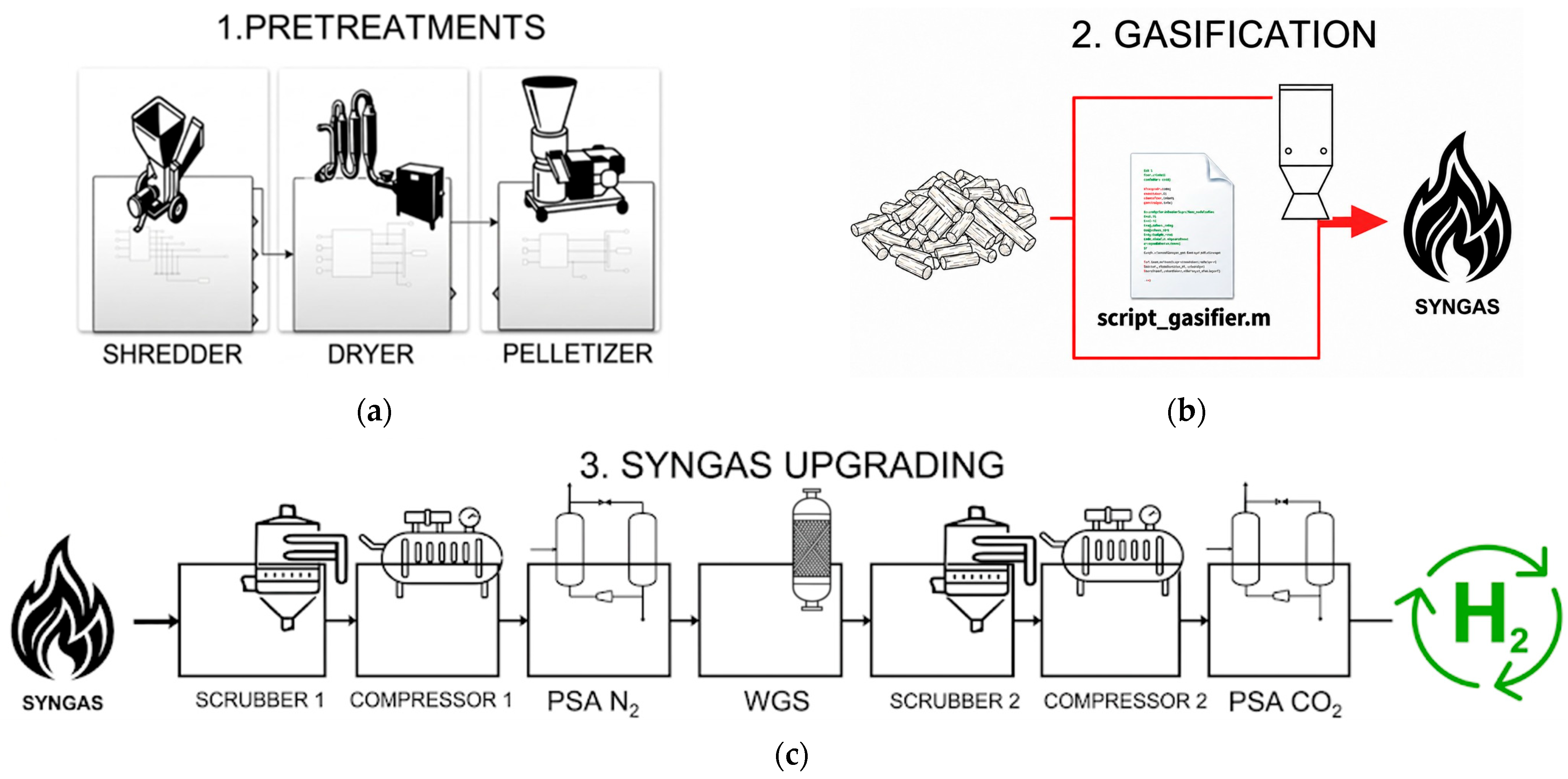
In the following section, the complete model will be used in order to simulate each process of the valorization chain. In particular, the different results obtained using the four different feedstock scenarios discussed in the introduction will be shown: scenario A (only vine prunings); scenario B (only grape stalks from a winery in Carpi); scenario C (a mix of prunings and grape stalks from the Carpi winery); and scenario D (only grape stalks from six wineries). First, it is useful to quantify the differences among the various scenarios listed. It can be observed that the mass of grape stalks in case B (159.29 ton/year) is approximately one-third of that in case D (492.73 ton/year); since in scenario C the model calculates the properties of the incoming biomass as a weighted average of the properties of grape stalks and prunings, the limited quantity of the former (the mass increase is 4.7%) suggests that they produce negligible differences in the results with respect to scenario A.

In

Table 3. Proposed model input parameters.

Model Input Data	Scenario A	Scenario B	Scenario C	Scenario D
Wood chipper fixed size (kg/h)	500	50	500	100
Wood chipper operating speed (rpm)	2500	2500	2500	2500
Dryer fixed size (kg/h)	350	50	350	50
Pellet mill nominal power (kW)	7.5	2.5	7.5	2.5
Gasifier size (input pellets) (kg/h)	200	25	200	25
Gasifier operating period (h)	7500	7500	7500	7500
Gasifier throat diameter (cm)	20	20	20	20
AFR (air/biomass) (-)	1.3	1.3	1.3	1.3
SFR (steam/biomass) (-)	0.5	0.5	0.5	0.5
O2 content in the introduced air % (vol)	31.5	31.5	31.5	31.5

, input parameters for the Fantasia model are shown.

Regarding equipment sizing, an iterative procedure is employed that accounts for the possibility of diverting part of the produced syngas to meet the system’s self-consumption. An initial simulation, based on estimated input parameters, provides the minimum required sizes of the devices and a preliminary assessment of the energy flows. From these results, a first self-consumption percentage is defined according to the syngas production and the hydrogen demand. A second value, representing the percentage required for the system to be energetically autonomous, is then calculated. If the two values differ, a new simulation is performed using the updated self-consumption percentage, and the procedure is repeated until convergence is reached.

This estimate is essential because the most energy-demanding components are the syngas compressors used in the PSA units, whose power consumption depends on the processed molar flow; higher syngas extraction thus increases energy demand. After determining the self-consumption associated with the minimum-size configuration, commercially available machines with comparable capacities are selected, and the iterative process is repeated to determine the real self-consumption percentage. Comparing the ideal and real values allows assessment of how the choice of equipment influences overall energy consumption.

In

Table 4. Results of sizing procedure.

Variable	A	B	C	D
Annual producible wood chips quantity (ton/year)	2372.4	111.5	2483.9	344.9
Annual pellets yield at 8%wt of moisture (ton/year)	1240	30	1270	80
Annual biomass availability (ton/year)	3390	160	3550	495
Min. size of chipper (kg/h)	451.89	21.24	473.13	65.69
Min. size of dryer (kg/h)	316.33	14.87	331.19	45.99
Min. size of gasifier (kg/h)	165.24	3.54	168.79	10.96
Power required for grinding at min. size (kW)	3.69	0.22	3.91	0.69
Power required for drying at min. size (kW)	71.99	8.79	80.78	27.19
Power required for pelletizing at fixed size (kW)	6.2	0.35	6.33	1.1

, the results of the first iteration of said sizing procedure are shown.

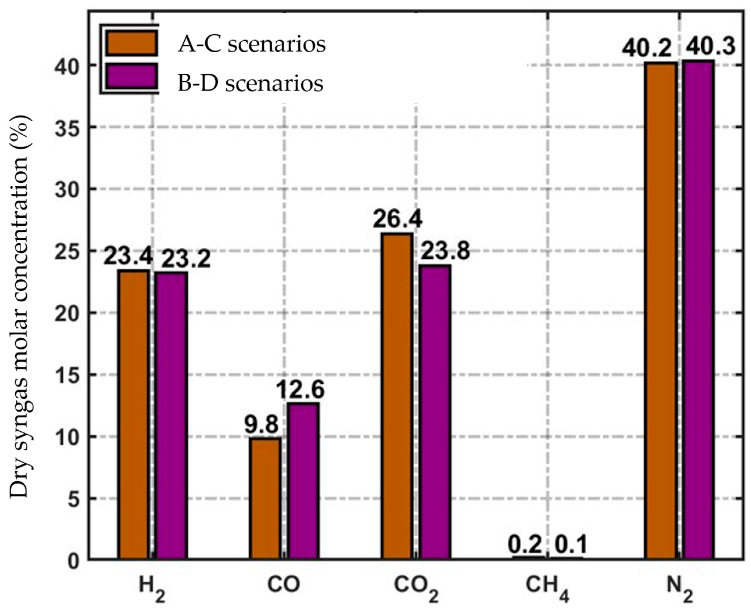
The composition of the produced syngas depends on the process variables and on the composition of the biomass but not on the size of the machinery, their nominal power, or the operating regime of the shredder. For this reason, it is also possible to evaluate the gas composition at this stage of the discussion. It was decided to group the four scenarios listed above into pairs, since scenarios A and C have a negligible difference in mass and lead to the same results, as happens for scenarios B and D. Figure 2 shows the molar concentrations of the main components of syngas in scenarios A–C and B–D.

It can be observed that the two pairs of scenarios produce syngas with almost the same concentration of H₂, CH₄ and N₂. The main differences lie in the concentration of CO and CO₂. In the case of carbon monoxide, grape stalks alone produce higher concentrations: this can be explained by the fact that they possess a higher carbon fraction and therefore favor the Boudouard reaction, which converts CO₂ into CO, leading to a greater production of carbon monoxide compared to the case of prunings alone. The opposite can be said for carbon dioxide, which is produced in greater amounts in the scenario with prunings only: these, in fact, are characterized by a higher oxygen content compared to stalks, thus leading to more extensive oxidations and consequently to a greater generation of CO₂. Clearly, the identified composition influences the performance of the subsequent processes and, consequently, the energy potential of the gas.

Once all the input parameters have been set as described so far and the sizing procedure is repeated until convergence is reached, results are obtained for the four scenarios A, B, C and D, which can be summarized as shown in

Table 5. Summary of the results obtained in each scenario.

Variable	A	B	C	D
Dry syngas higher heating value (MJ/Nm3)	4.29	4.59	4.3	4.59
Total syngas volume producible (Nm3)	1.56 × 106	2.10 × 105	1.56 × 106	4.20 × 105
Volume of bled syngas (Nm3)	3.81 × 105	1.05 × 105	3.82 × 105	1.32 × 105
Percentage of syngas volume used for balancing the system energy consumption (%)	24.44	49.9	24.45	31.25
Total Hydrogen yield (Nm3)	6.57 × 105	6.24 × 104	6.61 × 105	1.71 × 105
Estimated purity for the produced Hydrogen (%)	93.6	93.8	93.6	93.8
Specific Hydrogen production (Nm3/kgpellet)	0.53	2.35	0.52	2.08
Hypothetical syngas bleed fraction (%)	24.44	49.90	24.45	31.35
Compressor electric power consumption (kW)	22.22	2.01	22.32	5.51
Total thermal power required (kW)	4.59	11.83	4.91	11.83
Total electric power required (kW)	32.16	4.65	32.22	8.29
Useful recoverable thermal power (kW)	4.55	11.83	4.88	11.83
Useful recoverable electric power (through an ORC cycle) (kW)	17.07	0.22	17.06	2.70
Electric power obtained from the self-consumed syngas (kW)	15.13	4.45	15.24	5.59
Total power deficit (kW)	0.0041	−0.0091	−0.033	0.014
Syngas volume to be bled to balance consumption (Nm3)	3.81 × 105	1.05 × 105	3.82 × 105	1.32 × 105
Syngas bleed fraction required to balance consumption (%)	24.44	49.89	24.44	31.35

. In the considered model, convergence was achieved in three iterations.

The total hydrogen yield in scenarios A and C exceeds that of B by an order of magnitude, despite allocating 25% of the syngas to internal energy needs. While cases B and D exhibit specific production rates (H₂ per kg of pellets) 4–5 times higher than A and C, the latter produce more in absolute terms due to the significantly higher mass of biomass processed. Furthermore, the advantage of a centralized collection strategy is evident: scenario D (multiple wineries) produces nearly triple the hydrogen of scenario B (single winery).

Scenario B presents the highest energy criticality, requiring nearly double the syngas for self-consumption compared to A and C. This necessitates a critical review of energy balance assumptions to identify the factors limiting efficiency in this configuration.

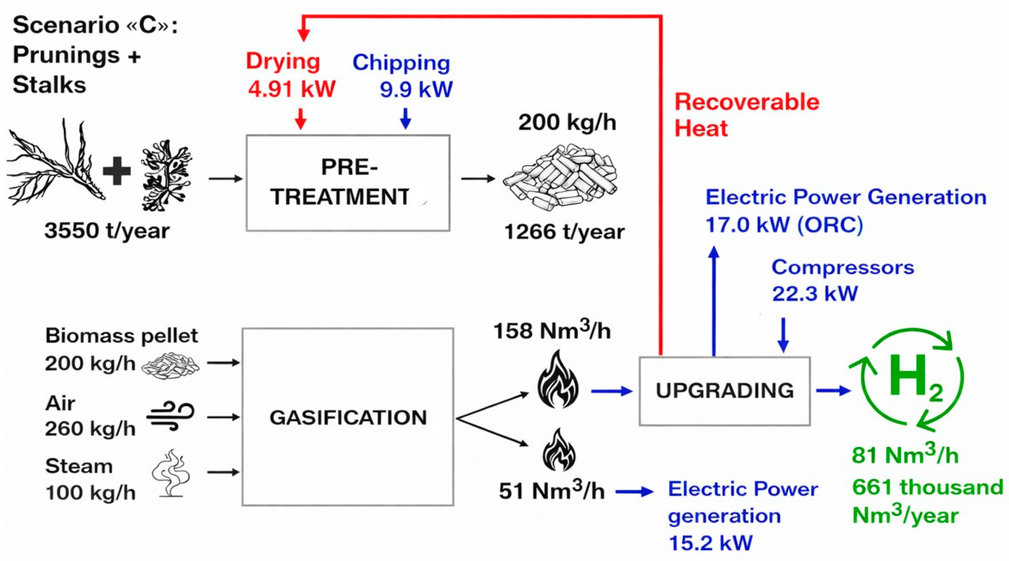
Syngas leaving the reactor undergoes cooling via a heat exchanger and scrubber. This recovered heat supports biomass drying, and any excess can power a 20 kW Organic Rankine Cycle (ORC) system for electric energy generation. However, ORC generation typically falls short of the plant’s total electrical demand, largely due to high-consumption compressors. Consequently, a portion of the extracted syngas must be diverted for power generation to ensure the plant’s energy self-supply, as summarized in Table 3.

Figure 3 shows the flow of energy and resources associated with scenario C.

Hypotheses A and C are the only ones that allow the extraction of syngas while still enabling the production of significant quantities of hydrogen. More demanding, but nevertheless potentially profitable, is the supply chain of case D, which, however, requires more than 30% of the syngas to be extracted. Scenario B is apparently unsustainable, in which half of the gas is extracted. Clearly, practical feasibility in these latter two scenarios requires a careful economic analysis, also taking into account the possibility of energy compensation through external sources.

Finally, an evaluation of the environmental sustainability of the supply chain is proposed through the quantification of greenhouse gas (GHG) emissions in comparison with traditional methods of hydrogen production, first and foremost, the SR of methane. This process involves the use of energy obtained through the combustion of part of the natural gas utilized, thus producing CO₂. In the case of gasification, on the contrary, various studies describe biomass-derived gasification as part of a carbon-neutral pathway, since the CO₂ released into the atmosphere was previously absorbed by plants during their lifetime [6]. Moreover, the remaining portion of the carbon contained in the biomass is sequestered in the form of biochar and therefore is not released into the atmosphere. The CO₂ emission balance was calculated by considering two contributions. The first corresponds to the emissions avoided with respect to the standard SR process of methane: these are quantified as 10 kg of CO_2,eq for every kg of H₂ produced [25]. The second considers the amount of CO₂ sequestered in the biochar. This can be quantified as follows:

$${\mathit{C}\mathit{O}}_{\mathbf{2},\mathit{e}\mathit{q}}=[\mathit{S}\mathit{p}\mathit{e}\mathit{c}\mathit{i}\mathit{f}\mathit{i}\mathit{c} \mathit{c}\mathit{h}\mathit{a}\mathit{r} \mathit{p}\mathit{r}\mathit{o}\mathit{d}\mathit{u}\mathit{c}\mathit{t}\mathit{i}\mathit{o}\mathit{n}]\cdot \mathbf{0.8}\cdot {\displaystyle \frac{\mathbf{44.01}}{\mathbf{12.01}}}$$

(6)

where the specific production of char quantifies the kg of char normalized with respect to the Nm³ of hydrogen produced, 0.8 is an estimate of the amount of carbon (in kg) contained in 1 kg of biochar, and finally, the ratio “44.01/12.01” is the stoichiometric ratio between the molar masses of CO₂ and C. The results of this analysis are reported in

Table 6. Third part of the simulated scenario results.

Variable	A	B	C	D
Avoided CO2 eq. Emissions (ton/year)	590.7	56.1	594.5	153.8
CO2 eq. sequestered in char (ton/year)	181.65	3.90	185.55	12.05
Total avoided/sequestered CO2 eq. (ton/year)	772.4	60.0	780.1	165.8
Total specific saving (kg/Nm3)	−1.18	−0.96	−1.18	−0.97

.

Scenario C offers the highest amount of CO₂ avoided in the atmosphere. In all the other cases, as well, there appears to be a saving of carbon dioxide. This result has one fundamental implication: gasification processes, if rightly designed, can be carbon-negative, since part of the carbon is segregated in the biochar and does not enter the carbon cycle in the atmosphere again. Clearly, this analysis only gives a first estimate of the ecological advantage of gasification with respect to traditional hydrogen production techniques. A cradle-to-gate LCA would be required to accurately quantify the carbon footprint of the process and to evaluate whether the system can legitimately be considered carbon-neutral or carbon-negative. In particular, such an assessment should also account for the CO₂ emissions associated with logistic operations and with the production of the equipment used in the overall chain, and assess with certainty the stability of the carbon stored in the biochar.

However, the results can be compared with those reported in the literature. The report “Biomass Gasification for Hydrogen Production” [26] indicates, for a supply chain comparable to the one considered in Fantasia’s analysis, a benefit in the range of 1.4–2 kg CO_2,eq/Nm³ of H₂. According to the proposed model, the highest specific CO_2,eq saving is achieved in scenario A, with a value of 1.18 kgCO_2,eq/Nm³ of H₂. This result is slightly below the range reported by [26]. Nevertheless, the assessment was based on largely conservative assumptions, which reasonably explain the lower values obtained.

3.4. Scenarios: Economic Analysis

Although the complexity of the overall system would require a comprehensive and detailed economic assessment, it is possible to estimate the investment and operating costs of the supply chain through an approximate approach. The methodology adopted in this study is based on the “scaling” technique, a well-established tool in process engineering economic analysis. Scaling consists of identifying reference processes available in the literature with known costs and comparable characteristics in terms of size, capacity, and productivity, and estimating the costs of the process under investigation as a function of those reference values through a power-law relationship. Using reference processes with dimensions too different from those of the proposed gasification process generally leads to unreliable estimates.

A reference was found in the study of Lv et al. [27], which considers a system capable of producing 240 Nm³/h of H₂ with a capacity of 200 kg/h of biomass. In scenarios A and C, it has been observed that the proposed gasification process can generate nearly 88 Nm³/h of H₂ by treating 200 kg/h of biomass. The size and process parameters are therefore similar and, as a first approximation, suitable for scaling. Nonetheless, the correlation between the proposed process and the reference one has clear limitations: first, Lv et al. [27] do not specify what pretreatment was considered and consequently which machines were used; second, Lv et al. [27] do not consider the PSA and SR units for syngas upgrading, restricting their analysis to the WGS post-treatment process. To address these two differences and balance the resulting error in the calculation, an additional percentage of the system costs is considered.

To start, the capital expenses (CAPEX) are computed. The process under analysis is correlated with that studied by Lv et al. [27] through the “six-tenths rule”, which is a power-law relationship with an exponent of 0.6. Lv et al. [27] estimate a CAPEX for the reference system of 2.55 million RMB (Chinese Renminbi) for the year 2007, when the analysis was carried out [27]. Through the six-tenths rule, the estimate for the process becomes 2.148 million RMB (at 2007 pricing). To update the costs of electrochemical conversion plants, the Chemical Engineering Plant Cost Index (CEPCI) is typically used. Finally, to convert into European currency, an exchange rate of 7.59 RMB/EUR is considered [28]. Finally, an additional 50% of the total cost was considered to compensate for the cost of components missing from the reference analysis. Moreover, the study by Lv et al. [27] considers the price of a PSA plant for oxygen production; this cost was considered to emulate the expense of the nitrogen removal unit. Overall, the estimated CAPEX amounts to 647 thousand euros.

Regarding the Operational Expenses (OPEX), that is, the costs necessary for the management and maintenance of the plant, the study by Lv et al. [27] considers labor costs, expenses for the purchase of biomass and energy, costs of consumable materials (catalysts), maintenance, and general expenses [27]. If the OPEX of the reference process were to be used for the proposed case as well, one would obtain an expenditure equal to one-third of the initial investment cost. This result appears unrealistic, considering that most estimates in the literature range between 3 and 6% of CAPEX [29]. It is therefore evident that, for the plant under consideration, the estimate by Lv et al. [27] cannot be regarded as applicable.

A simplified model was preferred, assuming only labor costs (including plant management, spare parts and maintenance) and costs related to catalysts. In the present study, an OPEX due to labor costs equal to 10% of CAPEX was adopted in order to remain conservative. Subsequently, an additional contribution to OPEX due to catalysts, equal to a further 10% of CAPEX, was considered. It should be noted that this value is also precautionary, since it has been shown that catalyst costs are around 7% of the initial investment costs. A total OPEX equal to 20% of the investment cost is thus obtained. This value still deviates from the typical range found in the literature; this can be justified by the conservative intent of the assumptions adopted. This results in OPEX amounting to 130 thousand euros per year.

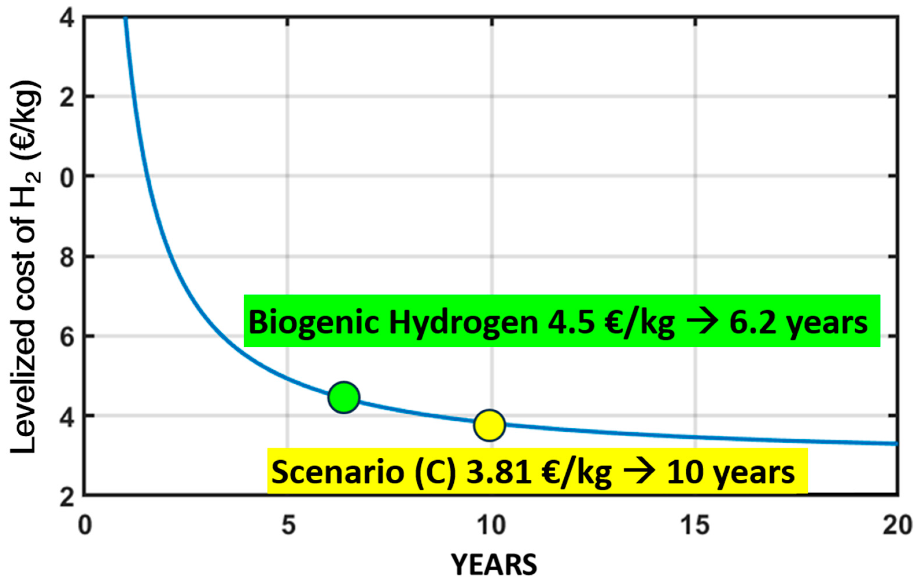
Once investment and operating costs have been calculated, it is possible to determine the price that must be assigned to hydrogen in order to repay the investment, defined as the breakeven price, considering a payback time of ten years. Through the calculation of the Net Present Value (NPV), considering a discount rate equal to 8% [30], it is possible to obtain the trend of the breakeven price as a function of time. The graph in Figure 3 summarizes the results obtained. It is found that, for a payback time of ten years, the breakeven price must be 3.81 €/kg. In the literature, it is reported that biogenic hydrogen from biomass reaches minimum prices between 2.48 and 2.70 €/kg [31] and a maximum threshold of 4.50 €/kg [32]; therefore, the breakeven price of the considered plant represents an economically advantageous solution.

A price of around 4.4 €/kg is a solution within the acceptable range and allows a payback period of less than seven years. In the case of a breakeven price of 4.5 €/kg, it can be calculated that the investment return time would be 6.2 years. A payback period of four years, on the other hand, proves to be too ambitious, since it would require prices higher than 5 €/kg. These results were calculated considering scenario C, that is, a plant fed by a mix of vine prunings and grape stalks.

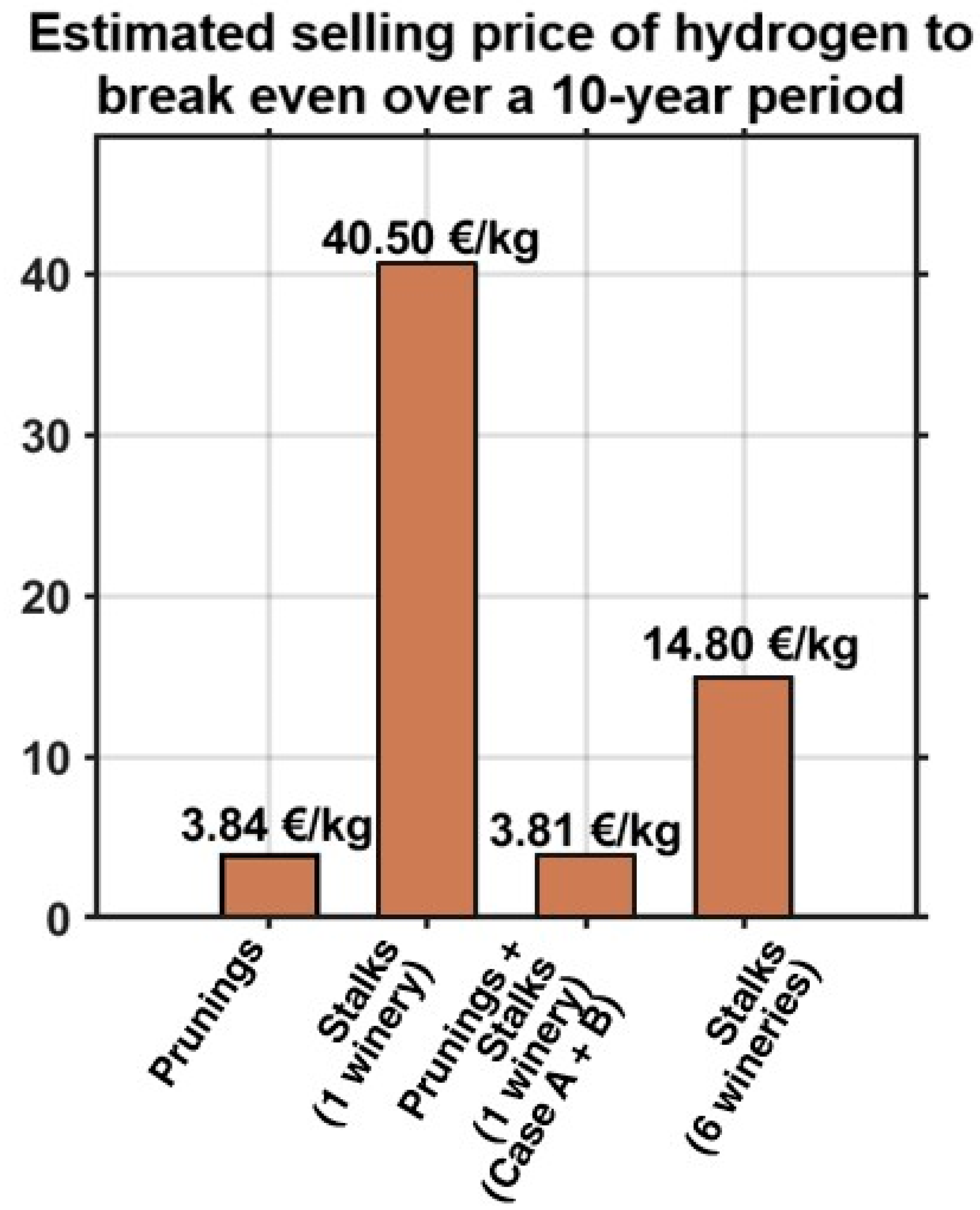
In Figure 4, the hydrogen prices required to achieve a system payback period of ten years are presented. These results highlight the importance of utilizing pruning residues as a feedstock in order for the process to become economically viable. Figure 5 shows the relationship between the selling price of the produced biogenic hydrogen and the payback period.

4. Conclusions

This study investigates an integrated system for converting viticulture residues, such as vine prunings and grape stalks, into biogenic hydrogen through gasification and advanced syngas upgrading stages. Using MATLAB-Simulink models, the research evaluates four different feedstock scenarios, namely scenario A (only vine prunings), scenario B (only grape stalks from the Carpi winery), scenario C (vine prunings + grape stalks from the Carpi winery), and scenario D (only grape stalks from six wineries), to analyze their technical efficiency, carbon-negative environmental impact, and economic profitability.

The results obtained show a satisfactory technical validity, ecological sustainability, and economic reliability of the valorization chain of agro-industrial residues of the wine industry. The comparative analysis of the process in the various feedstock scenarios shows how the use of vine prunings, with or without the addition of stalks, offers an excellent compromise between plant self-sufficiency and renewable hydrogen yield. Among the investigated cases, scenario C is the most advantageous overall, although its performance is very close to scenario A because the addition of stalks increases the annual feedstock mass by only 4.7%. Scenario C provides the highest hydrogen production (6.61 × 10⁵ Nm³/year), followed by scenarios A, D and B.

In particular, the valorization of biomass for the production of biogenic hydrogen has a dual advantage:

• The process is carbon-negative, as it is capable of producing a net reduction of CO₂, whose magnitude depends strongly on the selected scenario. The total avoided/sequestered CO₂ is 772.4 t/year in scenario A, 60 t/year in scenario B, 780 t/year in scenario C and 165.8 t/year in scenario D.
• The process is economically competitive in the pruning-based scenarios. For a payback time of ten years, the hydrogen selling price is 3.84 €/kg in scenario A and 3.81 €/kg in scenario C, while it rises to 14.8 €/kg in scenario D and 40.5 €/kg in scenario B. In addition, in scenario C, a selling price of 4.5 €/kg reduces the payback time to 6.2 years. These results indicate that scenarios A and C are the only clearly competitive configurations under the adopted assumptions, whereas the stalk-based cases are significantly less favorable.

Moreover, the developed MATLAB-Simulink model proved to be capable of predicting the behavior of the system with a degree of accuracy comparable to that of other models reported in the literature. At the same time, the main shortcomings of the adopted approach should also be acknowledged, since the model is based on equilibrium assumptions and does not fully account for reaction kinetics, tar evolution, reactor hydrodynamics, thermal losses, or fluctuations in fuel properties. These simplifications make the economic results subject to uncertainty. To improve the accuracy of the competitiveness assessment, future work should include a Monte Carlo analysis aimed at obtaining the probability distribution of the economic performance of the different scenarios.

Transition to renewable hydrogen in Europe will require the rapid expansion of electrolysis capacity, hydrogen transport and storage infrastructure, as well as additional renewable electricity generation; in this context, biomass-based pathways may represent a complementary option where local residual feedstocks are available [33].