Article

Interpretable Data-Driven Crystal Diameter Prediction in CZ Silicon Single-Crystal Growth via MIC-Guided and GWO-Optimized TCN–LSTM


1
E2 Growing Technology Department, Xi’an XINSEMI Material Technology Co., Ltd., Xi’an 710065, China
2
Growing Factory, Xi’an ESWIN Material Technology Co., Ltd., Xi’an 710114, China
3
School of Automation and Information Engineering, Xi’an University of Technology, No. 5 Jinhua South Road, Beilin District, Xi’an 710048, China
*
Author to whom correspondence should be addressed.
Processes 2026, 14(7), 1153; https://doi.org/10.3390/pr14071153
Submission received: 6 March 2026 / Revised: 21 March 2026 / Accepted: 1 April 2026 / Published: 3 April 2026
(This article belongs to the Section AI-Enabled Process Engineering)

Abstract

This study proposes a data-driven framework with post hoc interpretability analysis for one-step-ahead crystal diameter prediction in the Czochralski (CZ) silicon single-crystal growth process. To address the strong multivariable coupling, nonlinear dynamics, variable-specific delays, and difficulty of online measurement in CZ growth, the maximal information coefficient (MIC) was first used to screen key auxiliary variables from industrial process data. The Grey Wolf Optimizer (GWO) was then employed for multi-variable delay estimation and feature alignment, and a hybrid temporal convolutional network (TCN)–long short-term memory (LSTM) model was constructed to combine local temporal feature extraction with long-term dependency learning. Four input configurations were designed according to whether lag alignment and diameter history were included, and the proposed TCN-LSTM was systematically compared with standalone TCN and LSTM models. The results show that both diameter history and delay alignment improve prediction performance. Under the current single-run evaluation protocol, the TCN-LSTM configurations yielded lower prediction errors than the corresponding TCN and LSTM models under the same input settings. Under the withlag-withY configuration, the TCN-LSTM model achieved MSE = 0.00259, RMSE = 0.05087, MAE = 0.03949, and R2 = 0.96982. After GWO-based hyperparameter optimization, the best TCN-LSTM configuration further improved to MSE = 0.00239, RMSE = 0.04894, MAE = 0.03651, and R2 = 0.97207. SHAP-based analysis was further used to provide a post hoc interpretation of the relative contributions of key process variables to diameter variation. Overall, the proposed framework provides a data-driven prediction approach and may support subsequent process analysis and optimization in industrial CZ growth.

1. Introduction

Semiconductor-grade silicon single crystals are the core basic materials for the manufacture of integrated circuits and power devices. Large-size, high-quality silicon wafers are almost entirely obtained by processing single-crystal silicon ingots grown by the Czochralski (CZ) method. Feigelson et al. systematically reviewed the development of the CZ method in the semiconductor field based on the history of crystal growth and the theory of melt growth [1]. Vanhellemont reexamined the applicability of the v/G criterion in the defect control of large diameter silicon single crystals, pointing out that reasonable control of v/G is the key to obtaining defect-free crystals [2]. In actual production, the crystal diameter directly determines the number of silicon wafers that can be cut and the material utilization rate, and is also closely related to key quality indicators such as v/G value and oxygen content. During industrial CZ growth, the ingot diameter may fluctuate because of coupled thermal-field variation, melt convection, pulling-speed adjustment, and delayed process responses. Such diameter fluctuations directly affect downstream wafer slicing, material utilization, and dimensional consistency, and therefore have practical consequences for product quality and production stability. For the 12-inch CZ silicon ingot considered in this study, the target diameter is 304.8 mm, and the engineering objective is to keep the crystal diameter as stable as possible around this target and within a narrow control band during the steady-growth stage. This practical requirement motivates the development of data-driven prediction and control-support methods for CZ growth. Therefore, establishing a high-precision, online diameter prediction model around the industrial CZ single-crystal furnace is of great engineering significance for ensuring the quality, stability, and cost control of semiconductor silicon single crystal production [3].
The CZ silicon single-crystal growth process is essentially a dynamic system with multi-physics coupling, strong nonlinearity, and long time delays. Ren et al. pointed out that melt flow, electromagnetic stirring, and radiation convection conduction combined heat transfer work together at the solid–liquid interface, making the effects of heating power, pulling speed, and crystal/crucible rotation speed on diameter exhibit significant time-varying and multi-scale characteristics [4]. Wan et al. constructed a data-driven model predictive control framework based on the v/G quality index, showing that hybrid modeling in complex CZ processes helps improve quality control performance [5]. However, such work still mainly focuses on quality indices such as v/G, and the systematic prediction and analysis of crystal diameter, a key geometric variable, is relatively limited.
In terms of process monitoring and anomaly detection, Jiang et al. [6] proposed a node loss detection method and an anomaly identification framework using multi-modal data fusion, which significantly improved the fault detection capability of the CZ silicon single crystal growth process [7]. Liu et al. combined fuzzy C-means clustering with deep belief networks to propose a clustering learning modeling method for silicon single crystal growth, which was used for modeling and analyzing diameter and melt temperature under complex working conditions [8]. These studies show that multi-source data fusion and deep representation learning are helpful in characterizing the complex behavior of the CZ process, but they mainly focus on working condition identification or quality status classification, and still pay insufficient attention to multi-step prediction and interpretable modeling of continuous diameter time series.
In the broader field of process industries, deep learning-driven soft measurement methods have become a research hotspot. Sun and Ge conducted a systematic review of deep learning-based soft measurement, pointing out that deep networks have significant advantages over traditional machine learning methods in dealing with nonlinear, time-varying, and multi-condition problems [9]. Yuan et al. proposed a nonlinear dynamic soft measurement method based on supervised LSTM, which explicitly embeds time-series dependencies into the quality prediction model [10]. Zheng et al. further fused one-dimensional convolutional networks with LSTM to form a CNN-LSTM hybrid structure to improve the feature representation ability of industrial process soft measurement [11]. In another work, Yuan et al. designed an LSTM framework with a spatiotemporal attention mechanism for modeling soft measurement of complex industrial processes, which significantly improved prediction accuracy and robustness [12]. Regarding convolutional structures, Zhang et al. proposed a spatial-temporal attention-based TCN (STA-TCN) soft measurement model for predicting the quality of complex processes [13], while Zhou et al. embedded domain knowledge into a spatiotemporal deep LSTM framework to achieve soft measurement modeling under mechanistic constraints [14]. These results show that hybrid deep networks with convolutional and recurrent structures have good application prospects in modeling complex industrial processes.
On the other hand, variable selection and time delay estimation are equally important for multivariate time delay modeling problems. The Maximum Information Coefficient (MIC) proposed by Reshef et al. provides a unified measure for nonlinear correlation analysis of large-scale datasets and has been used in various fields to screen features that are highly correlated with the target variable from a large number of candidate variables [15]. The Grey Wolf Optimizer (GWO) proposed by Mirjalili et al. has been widely used in parameter optimization and multivariate time delay combination search due to its simple structure and strong global search capability [16]. Combining MIC and GWO to construct multiple time delay features suitable for CZ processes is expected to improve the discrimination ability of input features while ensuring physical rationality; however, there is currently a lack of systematic research on crystal diameter prediction.
With the widespread application of complex deep models in industrial scenarios, their “black box” problem has gradually become prominent, and Explainable AI (XAI) has therefore attracted attention. SHAP (SHapley Additive Explanations), proposed by Lundberg and Lee, unifies multiple feature importance measures based on cooperative game theory, and can quantify the contribution of each input variable to the model’s prediction results at both global and single-sample levels [17]. In sequence modeling, Bai et al. compared the performance of convolutional networks and recurrent networks in a series of sequence modeling tasks through a large number of experiments, pointing out that TCN has advantages in terms of effective memory length, training stability, and computational efficiency [18], while the LSTM model proposed by Hochreiter and Schmidhuber laid the foundation for various subsequent time series deep networks [19]. These studies show that structurally fusing TCN and LSTM [20], and supplementing them with interpretability tools such as SHAP, is expected to improve model transparency while maintaining high prediction accuracy. These works indicate that hybrid deep models and interpretability analysis have become an important research direction in Measurement and Control. However, for the growth process of semiconductor CZ silicon single crystals, especially for the key geometric variable of crystal diameter, there is still a lack of systematic research that integrates multivariable delay alignment, hybrid deep prediction, and interpretable analysis within a unified industrial data-driven framework.
  • It should be emphasized that the originality of this work does not lie in proposing new standalone algorithms for MIC, GWO, TCN-LSTM, or SHAP. Rather, it lies in developing a CZ-specific integrated framework that combines feature screening, variable-specific delay optimization, hybrid prediction, and post hoc interpretability for crystal diameter prediction using real industrial process data. The main contributions of this paper are summarized as follows: CZ-oriented delay-aligned input construction:
    To address the heterogeneous and variable-specific response delays in the CZ process, this study develops a delay-aligned input construction strategy that combines MIC-based feature screening with GWO-based multivariable lag optimization. The resulting inputs are more compact, physically interpretable, and better matched to the delayed influence of process variables on crystal diameter.
  • Unified comparative evaluation of prediction configurations:
    Based on the industrial CZ growth dataset, four input configurations were designed according to whether delay alignment and crystal diameter history were included. Under this unified setting, TCN-LSTM was systematically compared with standalone TCN and LSTM models, allowing the effects of delay alignment, diameter history, and hybrid architecture to be evaluated in a controlled manner.
  • Interpretable analysis of the best-performing model:
    SHAP was applied to the best-performing model to analyze the contribution and influence direction of key process variables on crystal diameter prediction. This provides an interpretable view of model behavior in the industrial CZ process and supports subsequent process analysis and optimization.

2. Process Description and Data Sets

2.1. CZ Silicon Single-Crystal Growth Process and Diameter Control

The Czochralski (CZ) silicon single-crystal growth process generally comprises melting the polycrystalline feedstock, thermal-field adjustment, seeding and necking, shoulder formation, constant-diameter growth, and tail-off. In practice, polycrystal-line silicon is melted in a quartz crucible to form the melt, and a quasi-steady thermal and flow field is established through external heating and, when applicable, magnetic confinement. During growth, the crystal is continuously withdrawn from the melt at a prescribed pulling rate, while the crystal and crucible rotate at different speeds to promote melt convection and homogenize the temperature distribution at the solid–liquid interface. In Figure 1, the target diameter serves as the setpoint for the outer diameter-control loop. The actual crystal diameter is the controlled output and is also fed back as a measured variable. The thermocouple signal is a measured variable used in the inner temperature-control loop. Pulling speed and heating power are manipulated variables generated by the control system. Disturbances are not explicitly shown in this simplified schematic; they mainly denote unmeasured thermal–fluid perturbations in the furnace, such as melt-convection fluctuations, thermal-field variations, and melt-level/interface changes.
Although the full CZ process includes all of the above stages, the modeling dataset used in this study does not cover the entire growth cycle; instead, it focuses on the post-shoulder steady growth interval, corresponding to the constant-diameter growth stage relevant to diameter prediction. These thermal–fluid mechanisms are not directly measured as standalone state variables in the industrial dataset; instead, they are indirectly represented by measurable process variables that influence the interfacial thermal and flow conditions, such as main heater power, crystal pull rate, crystal rotation speed, and crucible lift rate. A similar limitation applies to the melt-solid interface shape: although it is physically important for CZ growth, it is difficult to measure and register reliably in real time in the industrial environment, and was therefore not included as a directly observed variable in the present dataset.

2.2. Experimental Platform and Measurement Variables

The industrial dataset used in this study was collected from a large-diameter Czochralski (CZ) silicon single-crystal growth platform instrumented with multisource sensors, enabling real-time acquisition of thermal, mechanical, and electrical process variables. Accordingly, the proposed network was trained and evaluated using data acquired from real industrial Si single-crystal growth processes. However, the present validation was conducted offline on recorded industrial process data under a chronological train/validation/test protocol, rather than through online closed-loop deployment on the growth furnace.
After excluding non-informative signals, 15 effective auxiliary process variables were retained for subsequent correlation analysis. Table 1 summarizes the measured variables in the raw dataset (d22).
To further mitigate redundant inputs, we applied an MIC-based mRMR (maximum relevance–minimum redundancy) strategy. As a result, five variables were selected to form the optimal input set for the prediction model: crystal diameter history, crucible lifting rate, crystal pulling rate, crystal rotation speed, and main heater power.
These variables retain strong predictive power while maintaining low redundancy among themselves.
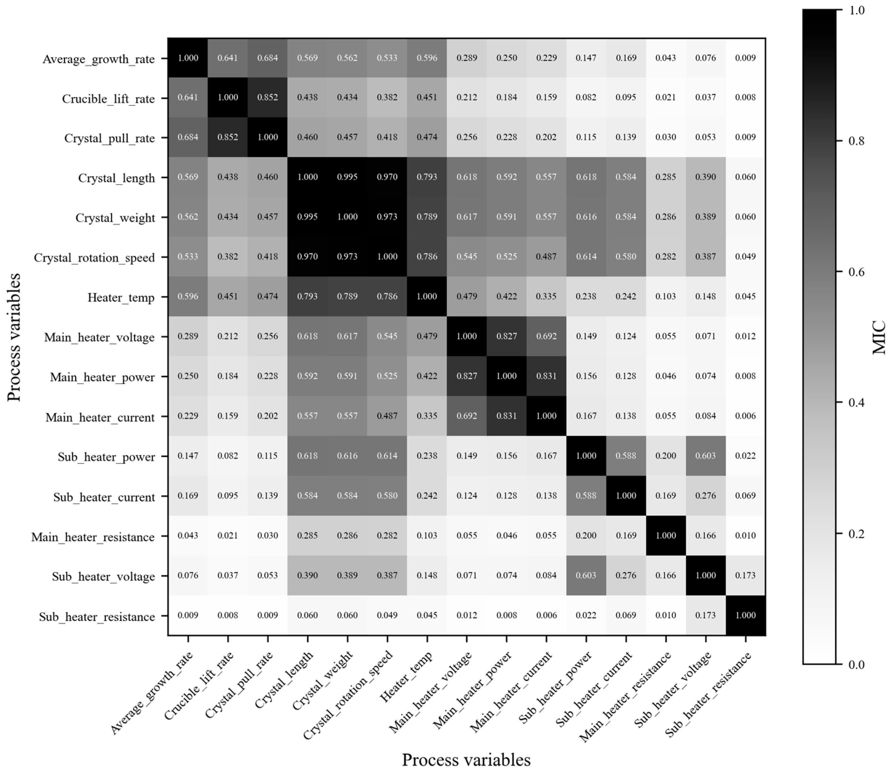
These selected variables also have clear physical relevance to the interfacial thermal–fluid behavior. Specifically, main heater power reflects the external thermal input and thus the overall thermal-field intensity; crystal rotation speed affects melt stirring and temperature homogenization near the solid–liquid interface; crystal pull rate influences the solidification rate and local heat-balance condition at the interface; crucible lift rate changes the melt level and the heater–melt–crystal geometric relationship, thereby affecting the thermal environment experienced by the interface. In addition, crystal diameter history captures the delayed integrated response of the interface evolution to these coupled thermal and flow mechanisms. Because these effects are not instantaneous, the subsequent lag-alignment step is used to represent their variable-specific delayed influence on crystal diameter (Figure 2).

2.3. Data Acquisition and Preprocessing

The raw dataset d22 was obtained from industrial crystal-pulling experiments. To reduce the influence of severe transients during the early and late stages of growth, the modeling dataset was restricted to the post-shoulder steady growth interval, i.e., the constant-diameter (equal-diameter) growth stage after shoulder completion and before the final tail-off stage. Therefore, stages such as melting, thermal-field adjustment, seeding and necking, shoulder formation, and tail-off were not included in the modeling dataset. During the retained interval, the crystal diameter remained within a controllable range, which improved the comparability and reliability of subsequent modeling and evaluation. To ensure the comparability and reliability of subsequent analyses, all signals were subjected to a consistent data-cleaning and preprocessing pipeline. In total, this study used one raw industrial dataset, denoted as d22. From d22, two derived modeling datasets were further constructed: d5, containing the selected key input variables, and d5_lag, containing the lag-aligned version of these variables for delay-aware prediction.
The raw industrial data used in this study were stored in the workbook 300mmData.xlsx, and the modeling data were extracted from Sheet2. The raw dataset contains 20,104 samples and 22 columns. The sampling interval is 2 s. The recorded variables include thermal, electrical, and mechanical process signals, together with the crystal diameter measurement. To improve modeling reliability, the data were first restricted to the post-shoulder steady growth interval, after which outlier removal was performed using the three-sigma rule, and all retained variables were normalized by min–max scaling.
For feature screening, the variables Time, Process, Argon flow setpoint, and Melt level were excluded from MIC analysis. MIC-based mRMR was then used to select five key auxiliary variables and construct the reduced dataset d5. Based on d5, variable-specific lag alignment was further applied to generate the delay-aligned dataset d5_lag for delay-aware modeling.
  • Outlier removal
Outlier removal was performed on the crystal diameter observation data using the three-standard-deviation principle. First, the mean and standard deviation μ of the crystal diameter data were calculated using the following formula:
μ = 1 n i = 1 n y i
σ = 1 n i = 1 n ( y i μ ) 2
where y i denotes i-th sample of the crystal diameter data, and n denotes the total number of samples.
The outlier threshold is determined using the three-sigma rule: the lower bound is set to a = μ 3 σ and the upper bound to b = μ + 3 σ . Any data points in the dataset that are smaller than a or greater than b are regarded as outliers and are removed from the dataset.
2.
Normalization
The collected auxiliary variables are normalized using the min–max scaling method. For the crystal diameter data, the maximum value y max and minimum value y min are first identified, and the original crystal diameter values are then linearly scaled to the interval [ 0 , 1 ] as follows:
y n o r = y y min y max y min + 10 12
where y n o r denotes the normalized data. The small constant 10−12 is introduced only for numerical stability, in order to avoid a zero denominator when y max = y min (or when the range becomes extremely small); its value is negligible relative to the scale of the measured variables and therefore does not affect the practical normalization results. The normalized data are subsequently used as the training data for the crystal diameter prediction model.
3.
Diameter prediction task and data partitioning
After preprocessing, the time series is reformulated as a supervised learning problem.
Let u t R p denote the vector of process variables at time t and let d t denote the corresponding crystal diameter. Given a historical window of length L and a prediction horizon H , the supervised learning task is formulated as a fixed-horizon direct forecasting problem. The input sample is constructed from the past L time steps of the selected process variables, while the prediction target is a single future diameter value:
x t = u t L + 1 , , u t
y t = d t + H
Under the withY configuration, the historical diameter sequence d t L + 1 : t is additionally included in the input; under the noY configuration, it is not included. In this study, H = 3 i.e., each sample predicts one future crystal-diameter value 3 sampling steps (6 s) ahead. By sliding the time window over the entire sequence, supervised sample pairs ( x t , y t ) are constructed.
To objectively evaluate model performance, the samples are partitioned in chronological order: the first 70% are used as the training set, the middle 10% as the validation set, and the final 20% as the test set. The training set is used for learning model parameters, the validation set for hyperparameter selection and early-stopping control, and the test set for the final performance evaluation, so that different models are compared under exactly the same data partition.

3. Methodology

To capture the nonlinear, multivariate, and strongly time-delayed characteristics of the CZ silicon single-crystal growth process, this study proposes a unified framework comprising multiple time-delay optimization, a TCN-LSTM hybrid model, and explainability analysis. The overall workflow can be summarized in four stages:
i.
Preprocessing of the raw industrial dataset d22 (300mmData.xlsx, Sheet2) and time-window reconstruction;
ii.
Variable screening to obtain the reduced input dataset d5 and multiple time-delay estimation and feature construction (MIC + GWO) to obtain the delay-aligned dataset d5_lag;
iii.
Training and evaluation of the TCN-LSTM model and comparative models based on d5 and d5_lag;
iv.
SHAP-based explainability analysis.

3.1. Multiple Time-Delay Estimation and Feature Construction

Because different process variables affect the crystal diameter with heterogeneous response delays, using the raw signals directly as model inputs can obscure these delay-dependent relationships. In this study, physically interpretable time-lagged features are constructed by combining correlation-based screening with multiple time-delay optimization.

3.1.1. MIC-Based Correlation Screening

Historical CZ single-crystal growth data are used to identify auxiliary variables that are most strongly associated with the crystal diameter using the maximal information coefficient (MIC).
The core idea of MIC is that, if two variables exhibit statistical dependence, then partitioning their scatter plot into a set of grids allows an empirical joint distribution to be approximated over the resulting bins, from which the mutual information can be computed. After normalization, the resulting score provides a quantitative measure of the association strength between the two variables.
MIC is built upon the concept of mutual information, which can be expressed as
I x , y = p x , y log 2 p x , y p ( x ) p ( y ) d x d y
where x and y denote the two variables, p ( x , y ) is their joint probability density function, p ( x ) and p ( y ) are the corresponding marginal probability density functions.
The MIC is then defined as
M I C ( x , y ) = max a b < B I ( x , y ) log 2 min ( a , b )
where a and b are the numbers of grid partitions along the x and y axes, respectively, and B is a user-specified upper bound, typically set to 0.6 power of the sample size. The value of MIC lies in [ 0 , 1 ] ; a larger MIC indicates a stronger dependence between the two variables.
The criteria for selecting key features based on MIC are as follows:
i.
Each selected feature should exhibit the strongest possible association with the crystal diameter; that is, its MIC with respect to the diameter should be maximized.
ii.
Meanwhile, redundancy among the selected features should be minimized; specifically, their pairwise MIC values should be as small as possible. Under these criteria, only auxiliary variables that are highly associated with the crystal diameter while exhibiting low inter-feature dependence are retained.
Based on the 22 collected process variables, including power, crucible lifting speed, crucible rotation speed, argon flow rate, crystal pulling speed, crystal rotation speed, thermal field temperature, main-chamber low vacuum, sub-chamber vacuum, main-heater voltage, main-heater current, main-heater resistance, crystal weight, crystal length, average growth rate, and crystal diameter, A Python program developed in Python 3.10.11 (Python Software Foundation, Wilmington, DE, USA) was used to compute the MIC between each of the first 15 variables and the diameter as well as the MIC among these 15 variables.

3.1.2. Multiple Time-Delay Optimization

According to the above MIC analysis, five features are selected; therefore, N = 5 in the following formulation. By sampling the time axis M is set to 6000, and the matrix is constructed as follows:
X = [ x 0 , x 1 , , x i , , x N ] = x 0 1 x 1 1 x i 1 x N 1 x 0 2 x 1 2 x i 2 x N 2 x 0 t x 1 t x i t x N t x 0 M x 1 M x i M x N M M × ( N + 1 )
Here, N = 5 denotes the five process variables, and M = 600 represents the 6000 sampling instants x 0 denotes the time series of the zero-delay reference variable, i.e., the target variable, and x i denotes the time series of the i-th process variable.
Assume that the multiple correlated time delays between the target variable and each process variable are represented by the delay vector.
Γ = [ τ 1 , τ 2 , , τ i , , τ N ]
where N = 5 .
In the original time-series data matrix, each process variable is sampled every 2 s, i.e., T = 2 . Thus, the time-delay parameters of the i-th process variable relative to the target variable must satisfy
Γ = D T = [ d 1 T , d 2 T , , d i T , , d N T ]
where T = 2 , D = [ d 1 , d 2 , , d N ] is the time-basis sequence, and d i is the time basis of the i-th process variable, which is a dimensionless integer. This formulation guarantees that the multiple correlated time-delay parameters of the process variables are integer multiples of the sampling period, thereby ensuring the feasibility of time-series reconstruction.
To estimate the multiple correlated time-delay parameters of different process variables, a temporal–spatial reconstruction of the time-series correlation matrix between each process variable and the target variable is performed under different time-basis sequences [20], so that the feedback information at different delays can be encoded by the time basis. The reconstruction procedure is as follows. First, a zero-delay reference variable x 0 is selected, and starting from time instant t , a sequence of F samples with sampling interval T is extracted to form the time series
x ˙ 0 = [ x ˜ 0 t , x ˜ 0 t + T , x ˜ 0 t + 2 T x ˜ 0 t , , x ˜ 0 t + ( F 1 ) T ] T
F T max τ 1 , τ 2 , , τ i , , τ N
so that the sequence contains at least one complete delay period and includes a transient state of the zero-delay reference variable.
According to the previously defined multiple correlated delay sequence, the delay coefficient of process variable x i with respect to the zero-delay reference variable is τ i ; thus, a new time series for x i is constructed by taking F samples starting from time t τ i i.e., from t d i T .
x ˙ i = x ˜ i t d i T , x ˜ i t + ( d i 1 ) T , x ˜ i t + ( d i 2 ) T , , x ˜ i t + ( d i ( F 1 ) ) T T
Because the new time series consists of F consecutive samples starting from t d i T and must cover at least one complete delay period, i.e., it must contain a transient state of the zero-delay reference (target) variable, F is set to 600 in this study.
Based on the time-delay parameters of each process variable, the spatiotemporal reconstruction yields the time-series correlation matrix X ˙ :
X ˙   = x ˜ 0 t x ˜ 1 t d 1 T x ˜ i t d i T x ˜ N t d N T x ˜ 0 t + T x ˜ 1 t ( d 1 1 ) T x ˜ i t ( d i 1 ) T x ˜ N t ( d N 1 ) T x ˜ 0 t + 2 T x ˜ 1 t ( d 1 2 ) T x ˜ i t ( d i 2 ) T x ˜ N t ( d N 2 ) T x ˜ 0 t + ( F 1 ) T x ˜ 1 t ( d 1 ( F 1 ) ) T x ˜ i t ( d i ( F 1 ) ) T x ˜ N t ( d N ( F 1 ) ) T F × ( N + 1 )
In the reconstructed time-series correlation matrix, the target variable is regarded as the parent sequence, and the multivariate process variables whose delay parameters are to be estimated are regarded as child sequences. The element-wise differences between the parent sequence and each child sequence are first computed and represented by matrix A :
A = a 01 a 0 i a 0 N a j 1 a j i a j N a ( F 1 ) 1 a ( F 1 ) i a ( F 1 ) N
where a j i = x ˜ 0 t + j T x ˜ i t ( d i j ) T ,   j = 0 , 1 , 2 , , 599 ,   i = 1 , 2 , , 5 .
Let a = min a j i and b = max a j i . The grey relational coefficient matrix is then denoted by γ :
γ = γ 01 γ 0 i γ 0 N γ j 1 γ j i γ j N γ ( F 1 ) 1 γ ( F 1 ) i γ ( F 1 ) N F × N
where γ j i = a + ρ b a j i + ρ b ,   j = 0 , 1 , 2 , , F 1 ,   i = 1 , 2 , , N . Here, ρ is the distinguishing coefficient; a smaller ρ implies stronger discriminating ability. When ρ = 0.5 , the grey relational coefficient matrix can better reflect the actual correlations among the multivariate variables; therefore, ρ = 0.5 is adopted in this study.
To describe the overall association between each child sequence and the parent sequence, the column-wise mean of the grey relational coefficient matrix is computed. The grey relational degree of the child sequences with respect to the parent sequence is defined as
r = [ r 1 , r 2 , , r i , , r N ] , r i = 1 F j = 0 F 1 γ j i
To quantitatively characterize the degree of multiple association between each process variable and the target variable in the reconstructed time-series correlation matrix, the overall correlation between the multivariate process variables and the target variable is described by the sum of the grey relational degrees, denoted by R , i.e.,
R = i = 1 N r i
The quantity provides a measure of the correlation among the multivariate time series in the time-series correlation matrix; a larger value indicates a stronger overall association. In this study, the GWO algorithm is employed to search for the maximum of R . When it reaches its maximum value, the corresponding set of multiple correlated time delays is regarded as the true multiple correlated delays of the CZ silicon single-crystal growth process.

3.2. TCN-LSTM-Based Crystal Diameter Prediction Model

Building on the historical data of silicon single-crystal growth, a crystal diameter prediction model denoted as TCN-LSTM is constructed by combining a temporal convolutional network (TCN) with a long short-term memory (LSTM) network [21]. The model hyperparameters are further optimized using the GWO algorithm. The TCN-LSTM model is employed to learn the nonlinear relationship between the auxiliary variables and the crystal diameter, which can be expressed as
d ^ t + H = f ( z t L + 1 : t )
where f(·) denotes the nonlinear mapping to be learned, Zt−L+1:t denotes the model input sequence constructed from the selected auxiliary variables, and, depending on the experimental configuration, may additionally include crystal-diameter history and/or lag-aligned variables. In this study, H = 3, i.e., the model predicts one future crystal-diameter value 3 sampling steps ahead, rather than a multi-output multi-step sequence.
The implemented TCN-LSTM model consisted of a TCN encoder, an LSTM predictor, and a linear output layer. Specifically, the TCN encoder contained two stacks of dilated residual blocks, with dilation factors (1, 2, 4, 8, 16) in each stack, kernel size 3, 128 channels per block, and dropout 0.05. The encoder output sequence was then fed into a two-layer LSTM with hidden size 128 and dropout 0.2, and the last hidden state was mapped to a scalar diameter prediction through a fully connected layer. Unless otherwise stated, the baseline TCN-LSTM was trained with a sequence length of 128, prediction horizon H = 3, batch size 64, AdamW optimizer, learning rate 5 × 10⁻⁴, weight decay 10−4, a maximum of 200 epochs, and early stopping patience of 15.
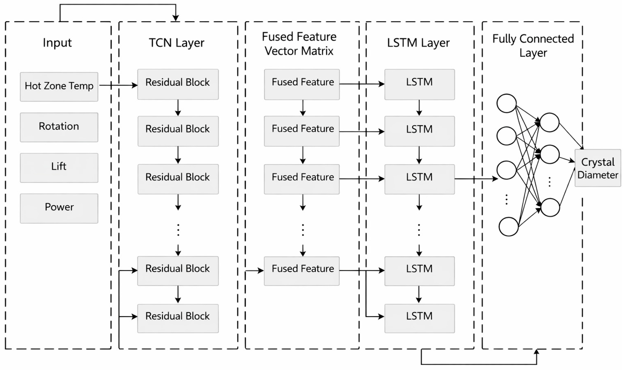
After obtaining the delay-aligned dataset d5_lag, it is necessary to construct a prediction model that can simultaneously characterize short-term temporal fluctuations and long-term dependencies. Leveraging the strength of TCNs in extracting multi-scale local features and the advantage of LSTMs in modeling long-range temporal dependencies, this study designs a serial TCN-LSTM hybrid architecture for crystal diameter prediction.

3.2.1. Overall Network Architecture

Let the input sequence be a delay-feature window of length L , denoted by X R L × d i n , where d i n is the input feature dimension. The overall architecture of the TCN-LSTM model consists of:
  • TCN feature-extraction module:
Composed of multiple one-dimensional dilated causal convolution layers with residual connections. It performs convolutions along the temporal dimension of the input sequence to extract multi-scale local temporal patterns and produces the feature sequence H T C N R L × d t c n .
ii.
LSTM temporal-modeling module:
Takes H T C N as input, and further model long-term dependencies via LSTM, yielding the hidden-state sequence H L S T M (or the last hidden state h t ).
iii.
Fully connected prediction layer:
Compresses the LSTM output into a vector and maps it through a fully connected layer to obtain the diameter prediction vector with horizon H , y ^ = d ^ t + 1 , , d ^ t + H During training, the mean squared error (MSE) is adopted as the loss function:
ι = 1 H i = 1 H d t + h d ^ t + h 2
The network parameters are optimized by backpropagation and gradient descent.

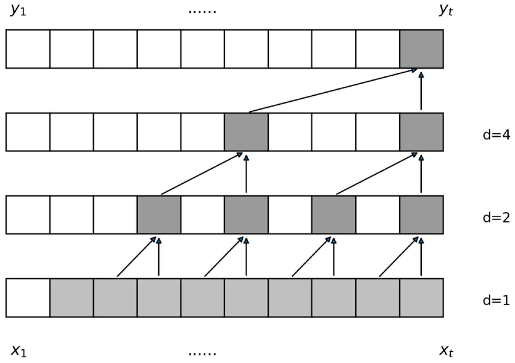
3.2.2. TCN Architecture: Residual Connections, Causal Convolutions, and Dilated Convolutions

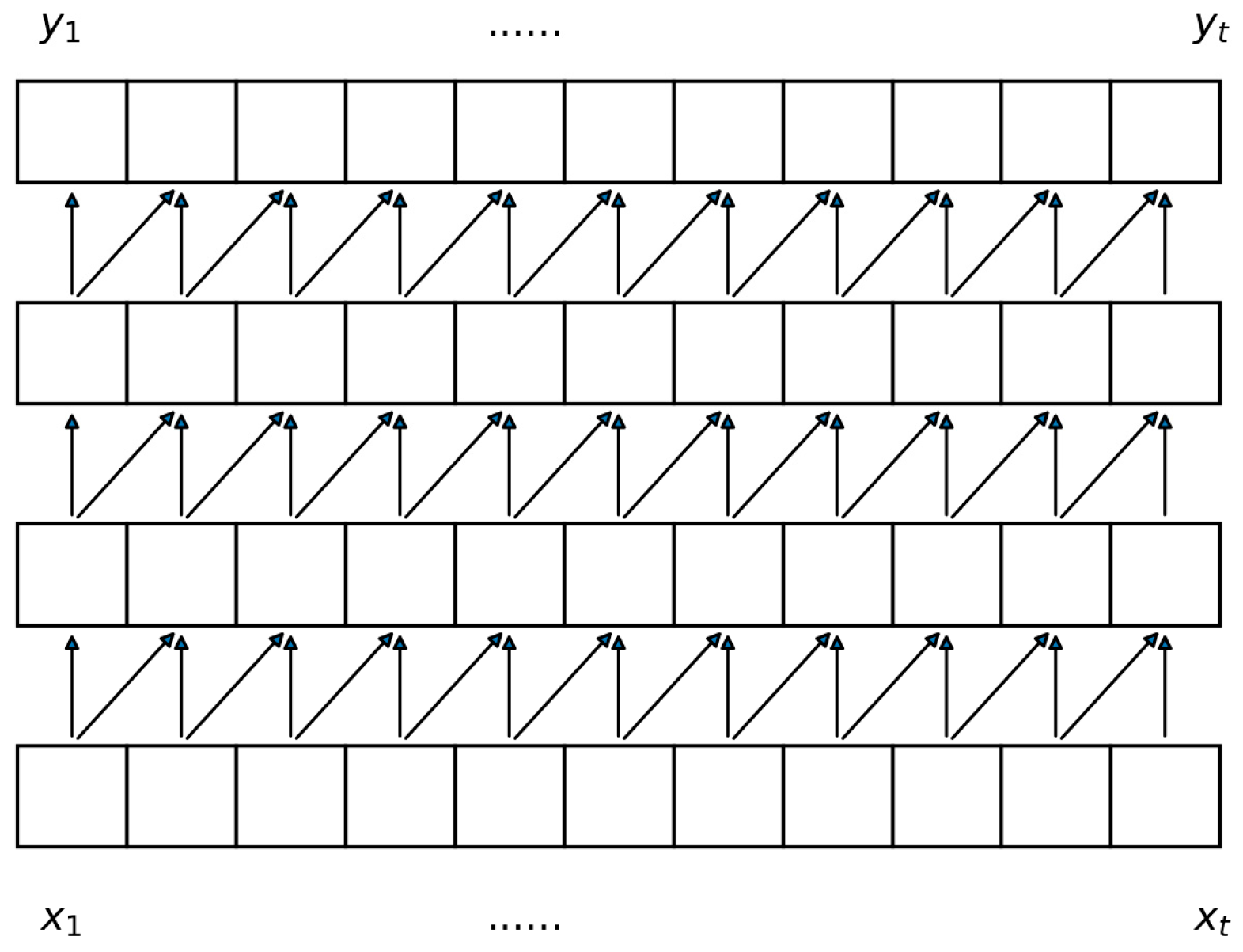
Causal convolution: at each layer, the value at time step t is determined only by the values at time steps t in the preceding layer (Figure 3, Figure 4 and Figure 5).
Causal convolution prevents information from future time steps from leaking into the present. The convolution kernel is defined over the current and past time steps of the sequence so that, for each time step, the output depends solely on the current and previous inputs.
Dilated convolution: the dilated convolution operation is defined as
F ( t ) = ( x f ) ( t ) = i = 0 k f ( i ) · x t d · i
where denotes the convolution operator, k is the kernel size, and a is the dilation factor. By inserting gaps between kernel elements, dilated convolution enlarges the receptive field with fewer layers in the network, thereby capturing long-range temporal dependencies.
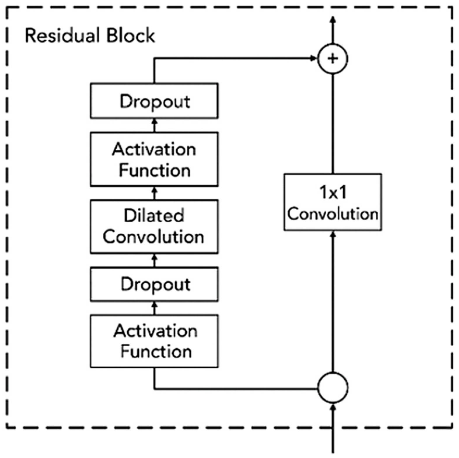
Residual connection: in each residual block, the input signal is passed through one or more convolutional layers and then added element-wise to the original input to form a residual connection. This residual connection helps alleviate the vanishing gradient problem and makes the training of deeper networks more efficient and stable. The computation can be written as
o = A c t i v a t i o n ( F ( x ) + x )
where F ( x ) denotes the output of the convolutional layers, x is the input, and A c t i c a t i o n ( ) is the activation function.

3.2.3. LSTM Sequence Modeling and Prediction Layer

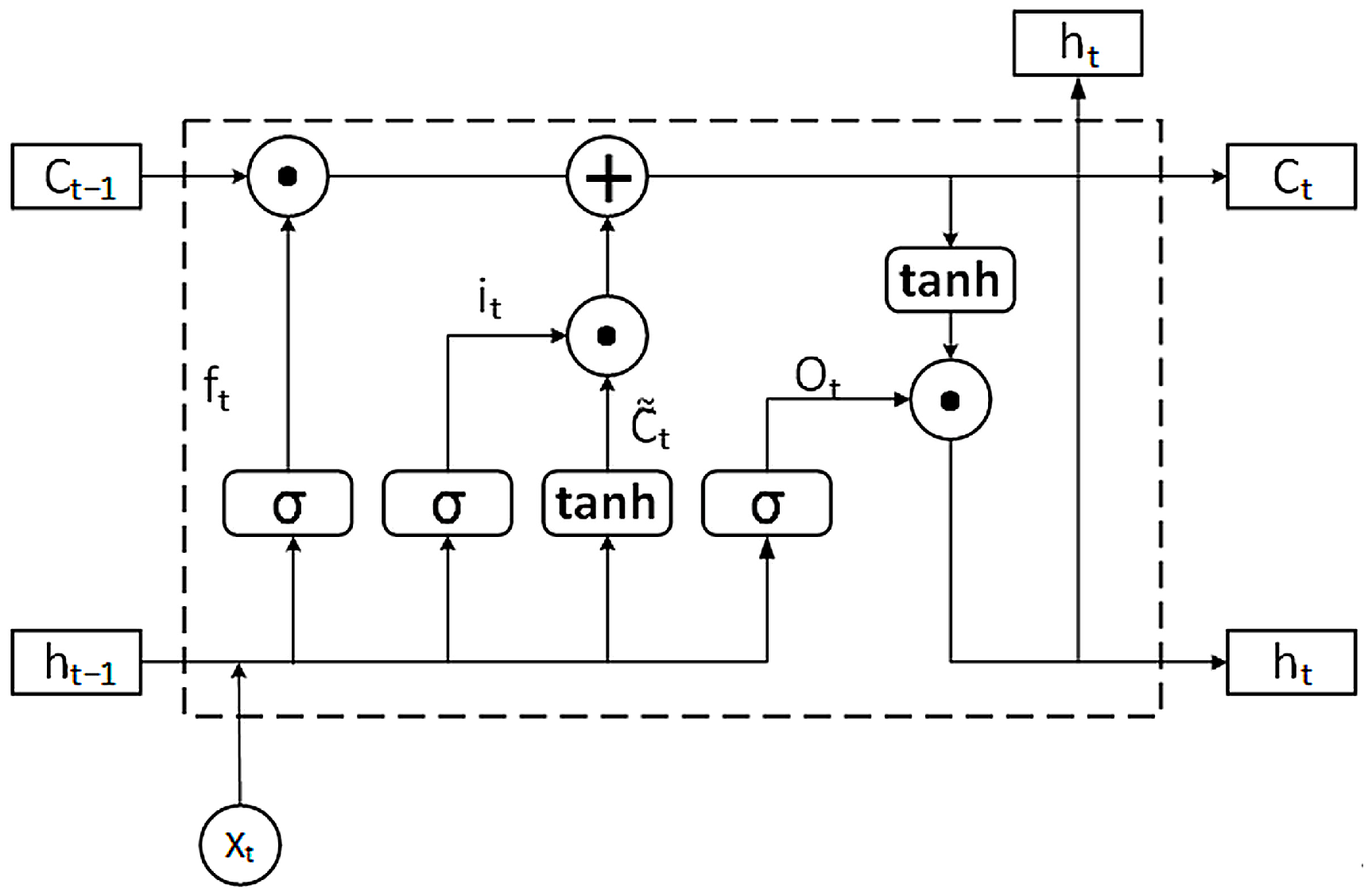
The memory cell consists of a forget gate, an input gate, and an output gate. For a given input, the computation in the memory cell proceeds as follows (Figure 6) [22].
  • Forget gate
The incoming information first passes through the forget gate, which determines how much of the previous cell state should be discarded. It is computed as
f t = σ [ W f ( h t 1 , x t ) + b f ]
where W f and b f are the weight matrix and bias vector of the forget gate, respectively, and σ denotes the sigmoid activation function. After the sigmoid operation, f t 0 , 1 ; a value close to 1 means “fully retained”, whereas a value close to 0 means “fully forgotten”.
ii.
Input gate
The input gate determines which new information will be written into the cell state:
i t = σ [ W f ( h t 1 , x t ) + b i ]
C ˜ t = tanh [ W C ( h t 1 , x t ) + b C ]
where W i , b i are the weight matrix and bias vector of the input gate, C ˜ t is the candidate cell state containing new information, and tanh ( ) denotes the hyperbolic tangent function.
iii.
Cell-state update
After deciding what to forget and what to remember, the cell state is updated as
C t = f t C t 1 + i t C ˜ t
where C t is the updated cell state and denotes element-wise multiplication.
iv.
Output gate
The processed information passes through the output gate to produce the hidden state h t :
O t = σ [ W O ( h t 1 , x t ) + b O ]
h t = O t tanh ( C t )
where W 0 and b 0 are the weight matrix and bias vector of the output gate, respectively.
Finally, a fully connected layer is applied to obtain the final prediction result (Figure 7). The computation of the fully connected layer is given by
y t = σ ( W y [ h t , h t ] + b y )
where W y is the weight matrix of the output layer, b y is the bias vector, and y t denotes the predicted crystal diameter.
  • TCN block: the input data sequence is first processed by a stack of TCN layers, where causal and dilated convolutions are employed to capture long-term dependencies in the sequence.
  • LSTM block: the output of the TCN block is fed into an LSTM block for feature fusion. The LSTM further processes the feature sequence produced by the TCN and, through its memory cells, captures complex temporal dependencies and sequential patterns.
  • Output layer: the output of the LSTM block is passed through a fully connected layer (or another suitable output layer) to generate the final prediction of the crystal diameter.

3.3. GWO-Based Hyperparameter Optimization for the TCN-LSTM Model

The hunting process of grey wolves is described as follows.

3.3.1. Encircling the Prey

In the GWO algorithm, the encircling behavior is modeled by the following position update equations:
D = C X p ( t ) X ( t )
X ( t + 1 ) = X p ( t ) A D
where D denotes the distance between a grey wolf and the prey, X ( t + 1 ) is the updated position vector of the grey wolf, X p and X are the position vectors of the prey and the grey wolf, respectively, and t is the current iteration index.
The coefficient vectors and are defined as
A = 2 a r 1 a
C = 2 r 2
where r 1 and r 2 are random vectors whose components are independently drawn from the interval 0 , 1 . The vector A is used to simulate the attacking behavior of grey wolves toward the prey. The parameter a is a convergence factor that decreases linearly from 2 to 0 as the number of iterations increases.

3.3.2. Chasing the Prey

During the iterative process, the α , β and δ wolves are used to guide the movement of each ω wolf so as to achieve global optimization. Given the positions X α , X β and X δ of the α , β , and δ wolves, respectively, the positions of all grey wolves are updated by
D α = C 1 X α X D β = C 2 X β X D δ = C 3 X δ X
where D α , D β and D δ denote the distances between an ω wolf and the α , β and δ wolves, respectively. The candidate positions influenced by these three leaders are then computed as
X 1 = X α A 1 D α X 2 = X β A 2 D β X 3 = X δ A 3 D δ
and the updated position of the ω wolf is obtained by averaging
X ( t + 1 ) = X 1 + X 2 + X 3 3
Here, X 1 , X 2 and X 3 represent the adjusted positions of the ω wolf under the influence of the α , β and δ wolves, respectively, and X ( t + 1 ) is the mean position used as its final updated location.

3.3.3. Attacking the Prey

In the following equation, t denotes the current iteration index and T is the maximum number of iterations. As a decreases linearly from 2 to 0, the corresponding components of A vary within the interval a , a . A larger value of a drives the grey wolves away from the prey, encouraging global exploration in search of potentially better prey; conversely, a smaller value of a pulls the wolves closer to the prey, promoting local exploitation. The parameter a is updated as
a = 2 2 t T

3.4. Explainability Analysis Based on SHAP

The SHAP algorithm is employed to interpret the crystal diameter prediction results. SHAP analysis was implemented in Python 3.10.11 using the SHAP package (version 0.49.0). For each sample, the Shapley value of every feature is computed to quantify its contribution to the model output. The Shapley value is defined as
ϕ i ( f ) = S N \ { i } S ! ( N S 1 ) ! N ! [ f ( S { i } ) f ( S ) ]
where ϕ i ( f ) denotes the Shapley value of the i-th feature, N is the set of all players (features), including feature i ; S is a subset of N that does not contain i ; S is the cardinality of S ; S N \ { i } represents all subsets of features excluding feature i and f ( S ) denotes the model prediction when only the feature subset S is present.

3.5. Evaluation Metrics

Given the true diameters in the test set { d i } and the corresponding predictions { d ^ i } , the evaluation metrics are defined as follows:
M S E = 1 N t e i = 1 N t e ( d i d ^ i ) 2
R M S E = 1 N t e i = 1 N t e ( d i d ^ i ) 2
M A E = 1 N t e i = 1 N t e | d i d ^ i |
R 2 = 1 i = 1 N t e ( d i d ^ i ) 2 i = 1 N t e ( d i d ¯ ) 2 , d ¯ = 1 N t e i = 1 N t e d i

4. Experimental Results and Analysis

This section provides a detailed comparison of the prediction results obtained under different models and input settings, explains the design rationale of the comparative and ablation experiments, and presents the corresponding evaluation metrics and visualization plots. We first summarize the predictive performance of each model under two binary factors—“whether time-delay information (Lag) is used” and “whether diameter history (Y_history) is used”—and then further analyze inter-model comparisons and hyperparameter optimization.

4.1. Experimental Setup and Metrics

For crystal diameter prediction, the following experimental setup is adopted. For each model (TCN-LSTM, TCN, LSTM), we consider two factors: whether time-delay alignment is introduced and whether historical crystal diameter values are used. This yields four configurations:
i.
no delay + no history.
ii.
no delay + with history.
iii.
with delay + no history.
iv.
with delay + with history.
All results reported in Table 2 correspond to the same fixed-horizon direct forecasting task with H = 3 , i.e., each input sample predicts one future crystal-diameter value 3 sampling steps (6 s) ahead; the four configurations differ only in whether lag alignment and diameter history are included. This design enables us to evaluate the impact of diameter-history information and temporal alignment (Lag) on model performance. Introducing diameter history aims to examine whether autoregressive information can improve prediction accuracy, whereas introducing delay alignment is intended to correct potential time-lag relationships between auxiliary variables and diameter. Under this setup, each model is trained and tested, and four evaluation metrics are computed: mean squared error (MSE), root mean squared error (RMSE), mean absolute error (MAE), and the coefficient of determination ( R 2 ). In the present study, GWO-based hyperparameter optimization was applied only to the proposed TCN-LSTM model. The standalone TCN and LSTM baselines were trained under fixed model settings and the same chronological data-partition/evaluation protocol, but did not receive an equivalent GWO search. All numerical values reported in Table 2 correspond to single-run results under the above chronological partition; repeated-run statistics, variance estimates, and formal significance tests were not included in the present study.
In this study, the term “robustness” is used in a limited comparative sense, namely, the consistency of relative model performance across the four predefined input configurations under the same dataset and evaluation protocol. It does not refer to statistical robustness established through repeated-run variance analysis, cross-dataset validation, or formal significance testing.
The following table summarizes the test metrics of all models under different configurations:
To assess the independent contribution of the delay-alignment module, matched-configuration comparisons were conducted while holding the use of diameter history constant. For TCN-LSTM, introducing lag alignment increased R2 from 0.68585 to 0.70594 under the noY setting and from 0.94587 to 0.96982 under the withY setting. Similar improvements were also observed for TCN (0.66416 to 0.75904; 0.81864 to 0.85124) and LSTM (0.52317 to 0.55927; 0.86383 to 0.96078). These results indicate that delay alignment provides a positive and independently observable contribution under the current dataset and evaluation protocol, although its effect is smaller than that of including diameter history in some settings. Therefore, the above comparisons should be interpreted as comparative single-run evidence under a fixed evaluation protocol, rather than as statistical significance claims.

4.2. Improvement Brought by Diameter History (Y_history)

For all models, incorporating the historical diameter markedly enhances predictive performance. For example, for TCN-LSTM without delay, adding diameter history increases R2 from 0.68585 to 0.94587; for LSTM without delay, R2 increases from 0.52317 to 0.86383. This indicates that the past states of the crystal diameter provide strong predictive information for its future evolution.

4.3. Improvement Brought by Delay Alignment (Lag)

Temporal alignment of the auxiliary variables also improves performance, although the gain is slightly smaller than that obtained from diameter history. For instance, for TCN-LSTM without history, introducing delay raises R2 from 0.68585 to 0.70594; on top of the history-enabled setting, adding delay further increases R2 from 0.94587 to 0.96982. This shows that explicitly modeling the temporal relationship between auxiliary features and the target can further enhance the model’s fitting ability.

4.4. Model Comparison

Regardless of whether history and delay are included, TCN-LSTM consistently outperforms the pure TCN and pure LSTM models. Under the same configuration, TCN-LSTM typically achieves the lowest MSE/MAE and the highest R 2 , demonstrating that the hybrid architecture, which combines convolutional feature extraction with memory mechanisms, is better suited to capturing complex temporal patterns.

4.5. Effect of Optimization

After applying grey wolf optimization (GWO) to tune the hyperparameters of TCN-LSTM, the model performance is further improved (e.g., R 2 increases to about 0.972), confirming the effectiveness of hyperparameter optimization in enhancing model accuracy.

4.6. Model Prediction Results

Plot the time-series comparison curves between the predicted values and the ground-truth values for each scenario.

4.7. TCN-LSTM: No Delay Alignment, No History vs. Has History

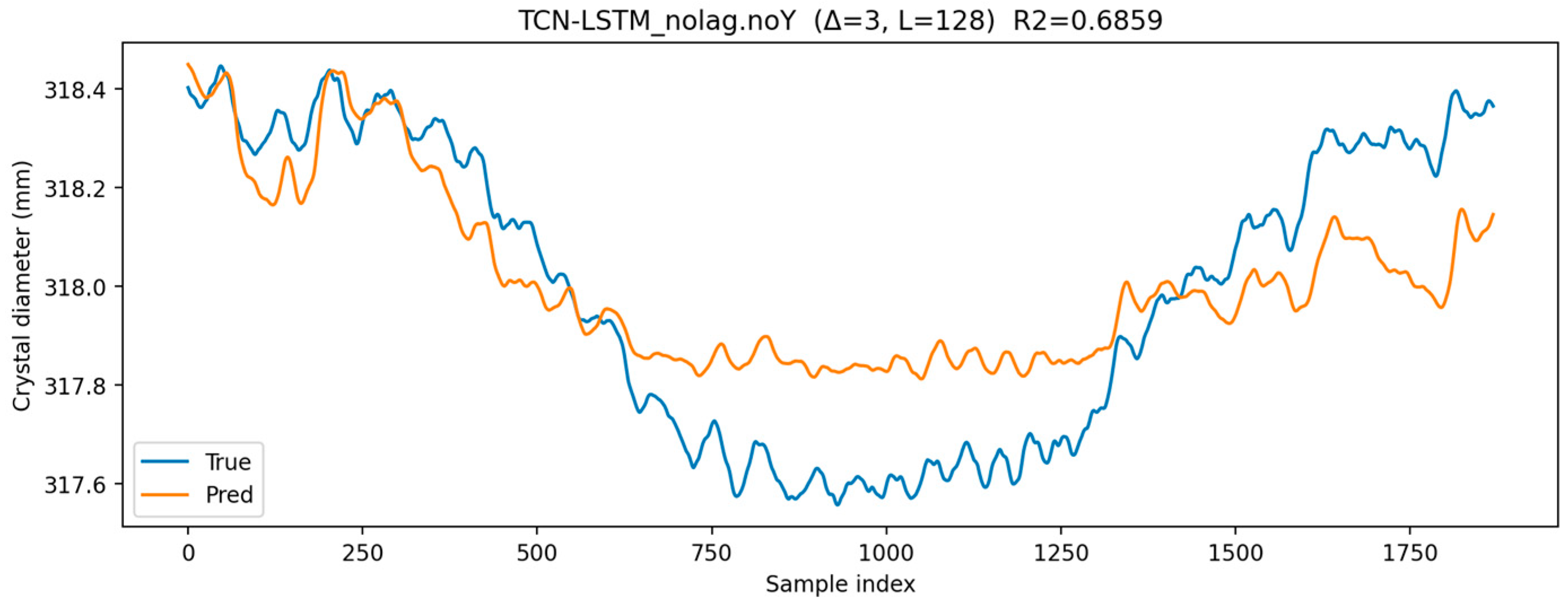
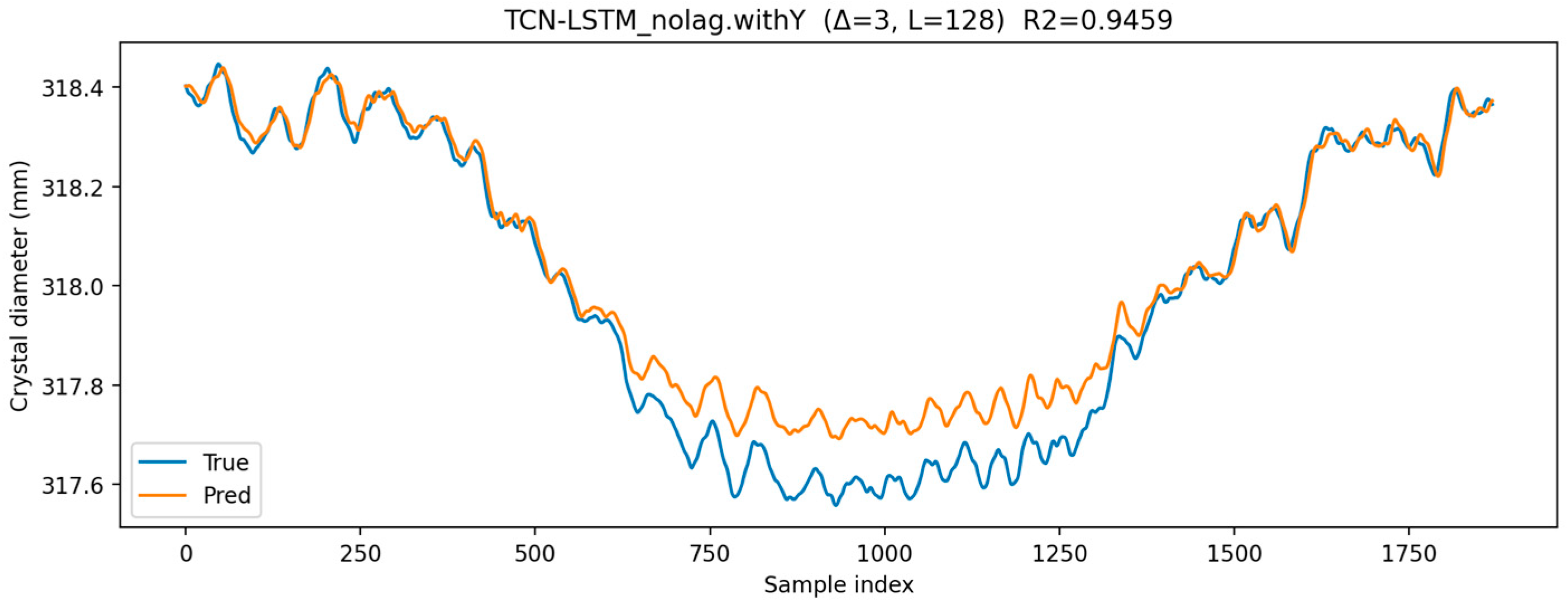
Without time delay and without historical data, the model only uses the current process variables for prediction, and the effect is generally poor. After adding the historical diameter (without time delay but with historical data), the model can access the past information of the target, and the fitting effect is greatly improved. Figure 8 and Figure 9 show the comparison curves of the prediction results under these two settings (horizontal axis is time step, vertical axis is crystal diameter).
The model is less able to capture trends under this setting, and the predicted curve deviates significantly from the actual curve.
After incorporating historical diameter data, the model’s predicted curve closely matches the actual value, the R2 value increases significantly, and the error decreases markedly, indicating that the addition of historical information effectively improves prediction accuracy.

4.8. TCN-LSTM Delay Alignment Comparison

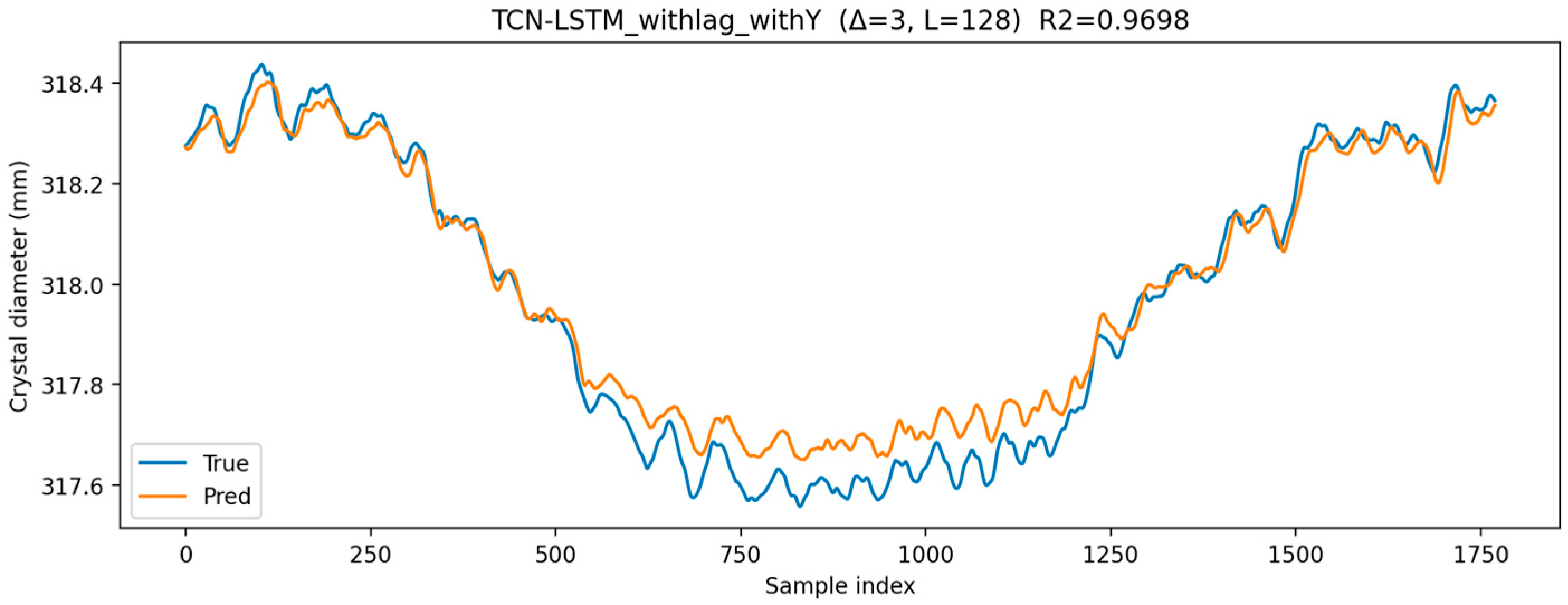
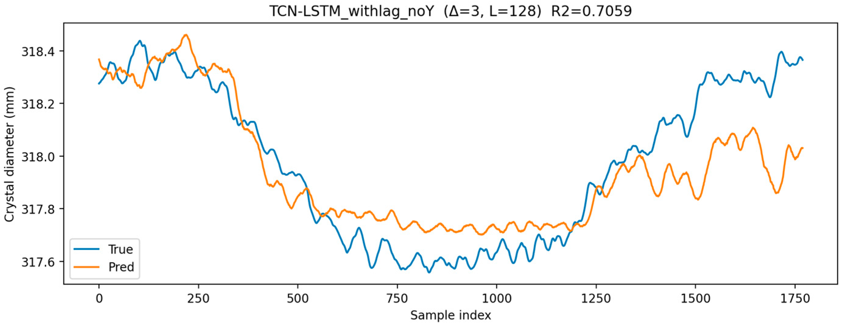
TCN-LSTM delay-alignment comparison: To evaluate the effect of delay alignment under the TCN-LSTM setting, Figure 8, Figure 9, Figure 10 and Figure 11 together show the four TCN-LSTM input configurations. Among them, Figure 9 and Figure 11 compare the two matched configurations with history, namely, no delay + with history and with delay + with history. For completeness, Figure 8, Figure 9, Figure 10 and Figure 11 together show the four TCN-LSTM input configurations.
As can be seen, after introducing time delay alignment, the model prediction is more accurate, especially in some delayed response regions where the fit is better, and R2 increases from 0.946 to 0.970.

4.9. Comparison of Four Settings for TCN-LSTM

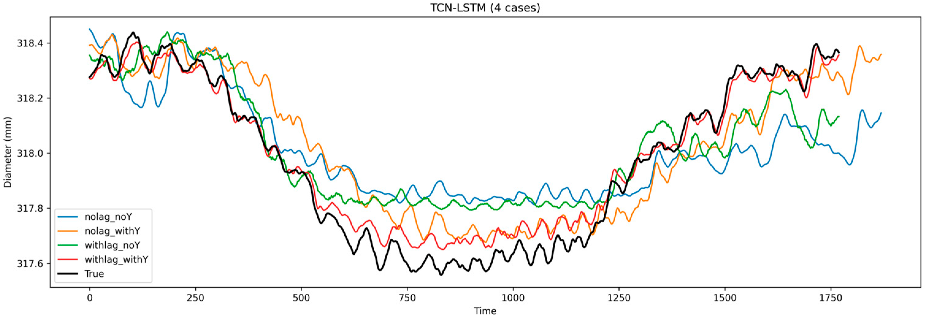
Without historical settings, the curve deviates significantly; with historical settings, it is closer to the true value, and adding delay alignment is slightly better than not adding delay alignment (Figure 12).

4.10. Results of TCN and LSTM Models

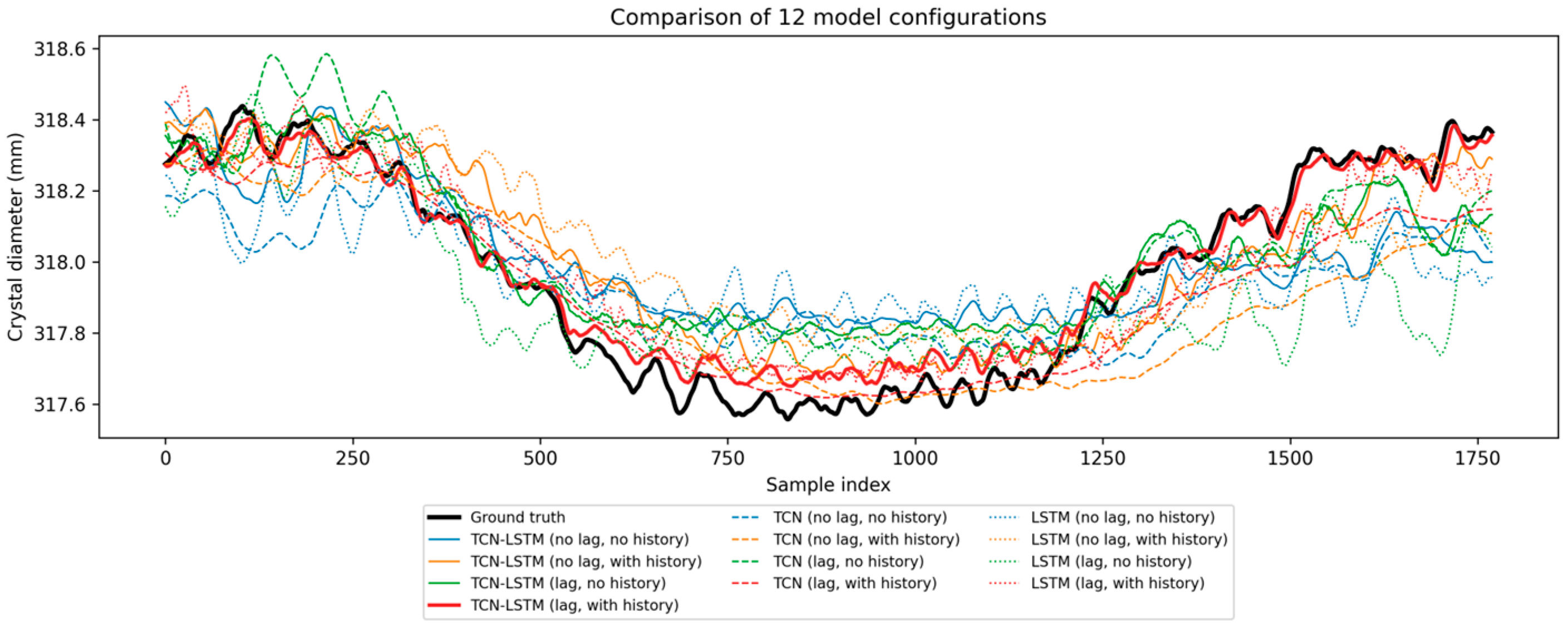
Similarly, prediction comparisons of the TCN and LSTM models under different settings were plotted. The results showed a similar trend to TCN-LSTM: performance with historical data was significantly better than without, and introducing delay alignment further improved the performance. For overall comparison, the prediction curves of the three models were summarized in the same figure (12 curves in total: 3 models × 4 settings), as shown in Figure 13.
As shown in Figure 13, the TCN-LSTM model provides the best overall fit among the three models, followed by TCN, while LSTM performs the worst under the compared settings. This figure summarizes all experimental scenarios and intuitively demonstrates the advantages and disadvantages of each approach.

4.11. Ablation Analysis and Interpretability

Based on the above results, the following observations can be drawn under the current single-run evaluation protocol. These comparisons provide comparative ablation evidence for the roles of diameter history, delay alignment, and model structure, but they should not be interpreted as strict statistical validation or tuning-balanced benchmarking.
(1)
The importance of diameter history: Diameter history information significantly improves predictive performance, indicating that the development of crystal diameter has its own continuity and predictable trend.
(2)
Independent contribution of delay alignment: Under the current dataset and evaluation protocol, introducing delay alignment yields consistent performance gains when compared under matched history settings. However, its contribution is smaller than that of including diameter history in some configurations.
(3)
Model structure differences: TCN-LSTM combines the advantages of convolution and recursion, and outperforms simple TCN or LSTM, while the pure LSTM model performs the worst when there is no history, showing that it is less sensitive to input features.
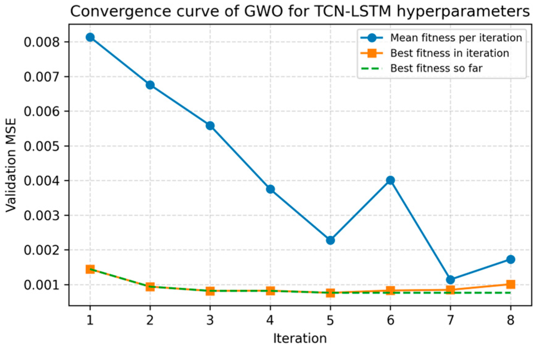
To understand the changing trend of the model’s prediction results, the Grey Wolf Optimization (GWO) algorithm was used to optimize the hyperparameters of the TCN-LSTM model. For the GWO-optimized TCN-LSTM model, the searched hyperparameters included the number of TCN channels, TCN kernel size, TCN dropout, LSTM hidden size, and learning rate. The search ranges were defined as follows: TCN_channels [96, 192] with a step of 16, TCN_kernel_size {3, 5, 7}, TCN_dropout [0.01, 0.30], LSTM_hidden [96, 192] with a step of 16, and lr [3 × 10⁻⁴, 7 × 10⁻⁴]. The LSTM depth and dropout were fixed at 2 layers and 0.2, respectively. For computational efficiency, GWO was run with 5 wolves and 8 iterations. Each candidate hyperparameter set was evaluated by training on a subset of the training partition (1000 samples) and computing the fitness on a subset of the validation partition (300 samples), using inner training for up to 8 epochs with patience 3. After the best hyperparameter set was identified, the selected TCN-LSTM model was retrained for up to 80 epochs with patience 8 before the final test evaluation. Accordingly, the GWO row in Table 2 should be interpreted as the optimized version of the proposed TCN-LSTM model, whereas the TCN and LSTM rows correspond to non-GWO baseline settings. Therefore, this study does not claim a tuning-balanced comparison against equally optimized baselines. Figure 14 illustrates the convergence process of the GWO algorithm:
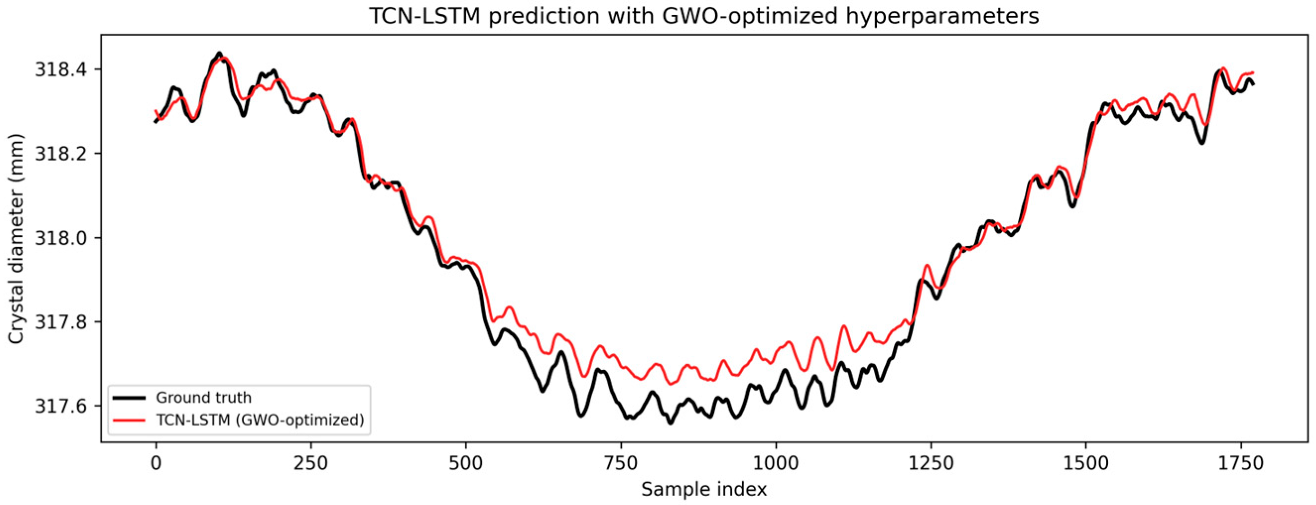
To verify the effectiveness of the optimization, Figure 15 further illustrates the prediction results of the TCN-LSTM after GWO.
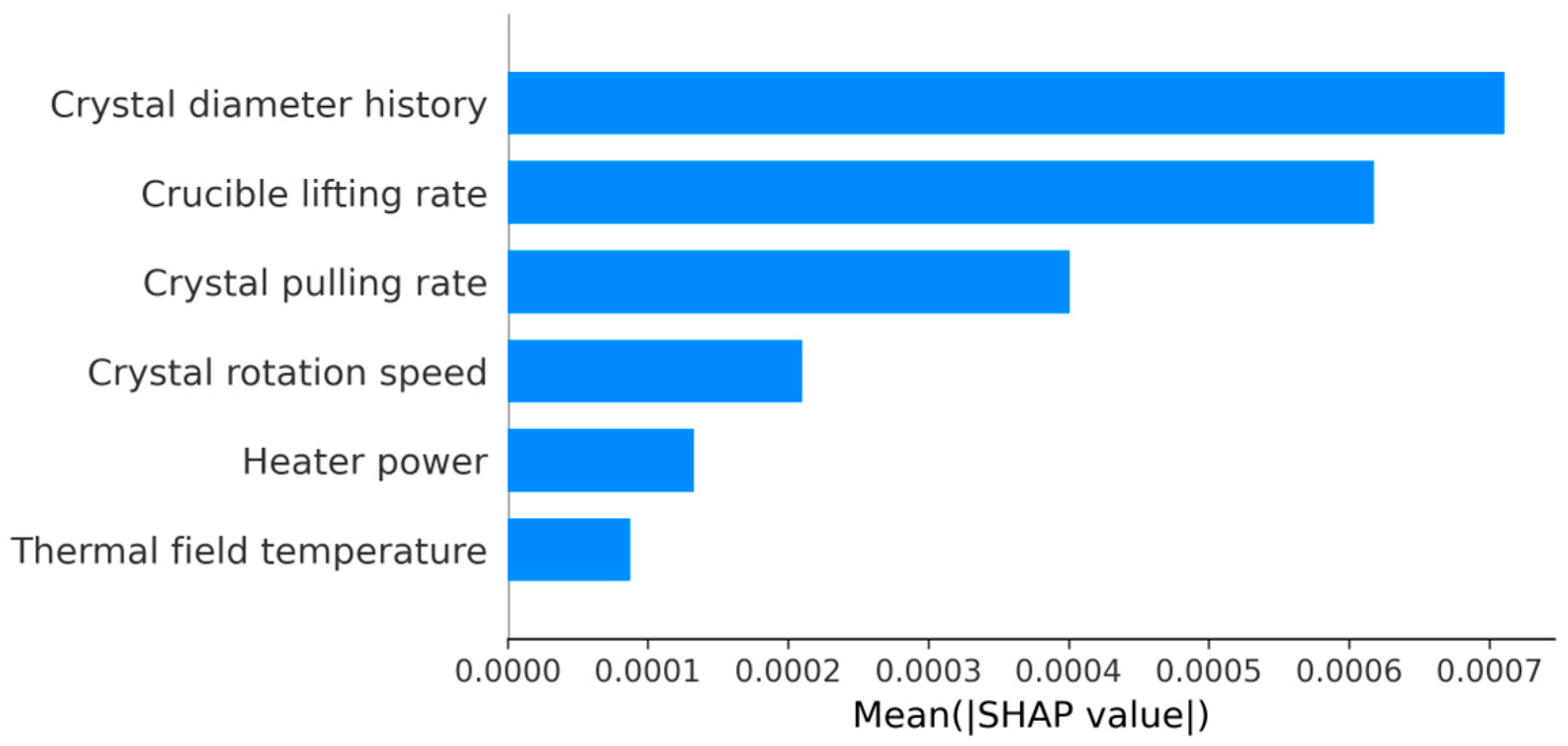
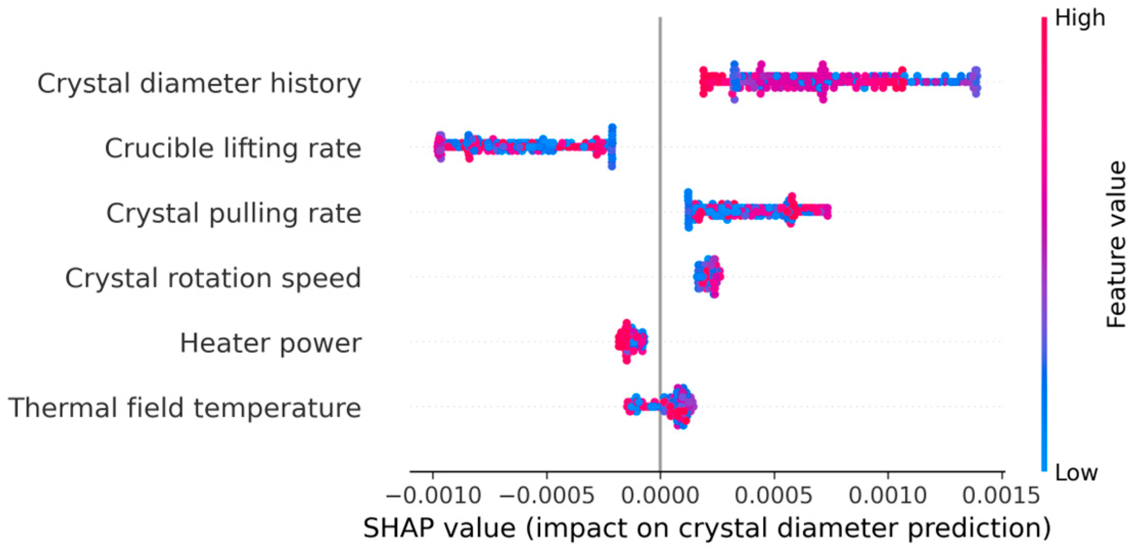
Finally, to explore the interpretability of the model, feature importance analysis (using SHAP values as an example) was performed on the optimized TCN-LSTM model. Figure 16 and Figure 17 show the histograms and bee colony diagrams based on SHAP, respectively, reflecting the contribution of each input feature to the prediction.
The SHAP summary indicates that features such as diameter history and crystal pull rate have relatively strong contributions to the model output, which is consistent with the preceding comparative results. This provides a post hoc explanatory view of the feature effects learned by the data-driven model. These results should be interpreted as predictive attribution within the trained model, rather than as direct identification of the underlying physical mechanisms of CZ growth. Among the technological variables listed in Table 1, crystal pull rate, crystal rotation speed, crucible lifting rate, heater power, and thermal-field temperature are the most influential process-related parameters under the current analysis. However, the present study is prediction-oriented and attribution-based; therefore, these results indicate relative predictive importance rather than a globally optimal set of process parameter values or operating setpoints.

5. Conclusions

The main findings of this study can be summarized as follows:
(1)
Under the current single-run evaluation protocol, the TCN-LSTM model showed the best predictive performance among the tested models across the four evaluated input configurations.
(2)
Quantitatively, under the withlag-withY configuration, the TCN-LSTM model achieved MSE = 0.00259, RMSE = 0.05087, MAE = 0.03949, and R2 = 0.96982, outperforming the corresponding TCN (R2 = 0.85124) and LSTM (R2 = 0.96078) models under the same input setting.
(3)
After GWO-based hyperparameter optimization, the best TCN-LSTM configuration further improved to MSE = 0.00239, RMSE = 0.04894, MAE = 0.03651, and R2 = 0.97207, which was the best result among all tested configurations.
(4)
When diameter history was held constant, delay alignment improved the TCN-LSTM performance from R2 = 0.68585 to 0.70594 under the noY setting and from R2 = 0.94587 to 0.96982 under the withY setting, indicating that both diameter history and delay alignment contribute positively to prediction performance under the current dataset and evaluation protocol.
(5)
SHAP-based analysis was used to provide a post hoc interpretation of the relative contributions of the input variables to the model output. These attribution results reflect the predictive behavior of the trained model and should not be interpreted as direct evidence for the identification of physical mechanisms.
It should be noted that the present study has several limitations. First, the analysis was conducted on a limited industrial dataset derived from one retained process sequence, so the dataset scope is still restricted. In particular, some physically meaningful but hard-to-measure state variables, such as the melt-solid interface shape, were not available in the present industrial dataset and therefore could not be explicitly incorporated into the model. Second, because some experimental settings explicitly include crystal diameter history, part of the predictive gain may depend on target autocorrelation, and the resulting performance should not be interpreted as relying solely on auxiliary process variables. Third, although TCN and LSTM were used as comparative baselines, stronger baselines and tuning-balanced benchmark models were not included in the present study. Fourth, the reported results are based on a fixed chronological partition without cross-run validation, repeated-run variance estimates, confidence intervals, or formal significance testing. Therefore, the current findings should be interpreted as comparative evidence under the present dataset and evaluation protocol, rather than as conclusive evidence of broader generalization. Future work should extend the dataset scope, include cross-run validation, adopt stronger and tuning-balanced baselines, and further examine the extent to which predictive performance depends on target autocorrelation. Accordingly, the present study should be understood as providing comparative evidence for the proposed integrated framework under the current dataset and evaluation protocol, rather than as definitive proof of novelty, robustness, or benchmark superiority.

Author Contributions

Conceptualization, D.L.; methodology, H.P. and P.Z.; software, P.Z.; validation, H.P. and C.X.; investigation, H.P.; data curation, P.Z.; writing—original draft preparation, H.P.; writing—review and editing, D.L. and C.X.; supervision, D.L. All authors have read and agreed to the published version of the manuscript.

Funding

This research was funded by the National Major Scientific Instrument Development Project of China under Grant 62127809.

Data Availability Statement

The data presented in this study are available on request from the corresponding author.

Conflicts of Interest

Author Hao Pan was employed by the company E2 Growing Technology Department, Xi’an XINSEMI Material Technology Co., Ltd. Author Pengju Zhang was employed by the company Growing Factory, Xi’an ESWIN Material Technology Co., Ltd. The remaining authors declare that the research was conducted in the absence of any commercial or financial relationships that could be construed as a potential conflict of interest. The E2 Growing Technology Department, Xi’an XINSEMI Material Technology Co., Ltd. and Growing Factory, Xi’an ESWIN Material Technology Co., Ltd. had no role in the design of the study; in the collection, analyses, or interpretation of data; in the writing of the manuscript, or in the decision to publish the results.

References

  1. Feigelson, R.S. Crystal growth history: Theory and melt growth processes. J. Cryst. Growth 2022, 594, 126800. [Google Scholar] [CrossRef] [Scilit]
  2. Vanhellemont, J. The v/G criterion for defect-free silicon single crystal growth from a melt revisited: Implication for large diameter crystals. J. Cryst. Growth 2013, 381, 134–138. [Google Scholar] [CrossRef] [Scilit]
  3. Wan, Y.; Liu, D.; Liu, C.; Ren, J. Data-driven model predictive control of Cz silicon single crystal growth process with V/G value soft measurement model. IEEE Trans. Semicond. Manuf. 2021, 34, 420–428. [Google Scholar] [CrossRef] [Scilit]
  4. Ren, J.C.; Liu, D.; Wan, Y. Modeling and application of Czochralski silicon single crystal growth process using hybrid model of data-driven and mechanism-based methodologies. J. Process Control 2021, 104, 74–85. [Google Scholar] [CrossRef] [Scilit]
  5. Wan, Y.; Liu, D.; Ren, J.-C.; Wu, S.-H. Study on the hierarchical predictive control of semiconductor silicon single crystal quality based on the soft sensor model. Sensors 2023, 23, 2830. [Google Scholar] [CrossRef] [Scilit] [PubMed]
  6. Jiang, L.; Xue, R.; Liu, D. Node-loss detection methods for CZ silicon single crystal growth based on multimodal data fusion. Sensors 2023, 23, 5855. [Google Scholar] [CrossRef] [Scilit]
  7. Jiang, L.; Wei, H.; Liu, D. Abnormal state detection of CZ silicon single crystal growth process based on multimodal fusion network. Sensors 2024, 24, 6819. [Google Scholar] [CrossRef] [Scilit] [PubMed]
  8. Liu, Y.; Liu, D.; Song, Z. Data-driven clustering learning modeling for semiconductor silicon single crystal growth process based on fuzzy C-means and deep belief network. Trans. Inst. Meas. Control 2025, 47, 1748–1761. [Google Scholar] [CrossRef] [Scilit]
  9. Sun, Q.; Ge, Z. A survey on deep learning for data-driven soft sensors. IEEE Trans. Ind. Inform. 2021, 17, 5853–5866. [Google Scholar] [CrossRef] [Scilit]
  10. Yuan, X.; Li, L.; Wang, Y. Nonlinear dynamic soft sensor modeling with supervised long short-term memory network. IEEE Trans. Ind. Inform. 2020, 16, 3168–3176. [Google Scholar] [CrossRef] [Scilit]
  11. Zheng, J.; Ma, L.; Wu, Y.; Ye, L.; Shen, F. Nonlinear dynamic soft sensor development with a hybrid supervised CNN–LSTM network for industrial processes. ACS Omega 2022, 7, 16653–16664. [Google Scholar] [CrossRef] [Scilit] [PubMed]
  12. Yuan, X.; Li, L.; Shardt, Y.A.; Wang, Y.; Yang, C. Deep learning with spatiotemporal attention-based LSTM for industrial soft sensor model development. IEEE Trans. Ind. Electron. 2021, 68, 4404–4414. [Google Scholar] [CrossRef] [Scilit]
  13. Zhang, L.; Ren, G.; Li, S.; Du, J.; Xu, D.; Li, Y. A novel soft sensor method for industrial quality prediction based on temporal convolutional network with spatial and temporal attention. Chemom. Intell. Lab. Syst. 2025, 257, 105272. [Google Scholar] [CrossRef] [Scilit]
  14. Zhou, J.; Yang, C.H.; Wang, X.L.; Cao, S.Y. Domain-knowledge-embedded spatio-temporal deep LSTM framework for soft sensor modeling in industrial processes. Eng. Appl. Artif. Intell. 2023, 126, 106847. [Google Scholar] [CrossRef] [Scilit]
  15. Reshef, D.N.; Reshef, Y.A.; Finucane, H.K.; Grossman, S.R.; McVean, G.; Turnbaugh, P.J.; Lander, E.S.; Mitzenmacher, M.; Sabeti, P.C. Detecting novel associations in large data sets. Science 2011, 334, 1518–1524. [Google Scholar] [CrossRef] [Scilit] [PubMed]
  16. Mirjalili, S.; Mirjalili, S.M.; Lewis, A. Grey wolf optimizer. Adv. Eng. Softw. 2014, 69, 46–61. [Google Scholar] [CrossRef] [Scilit]
  17. Lundberg, S.M.; Lee, S.I. A unified approach to interpreting model predictions. In Proceedings of the Advances in Neural Information Processing Systems, Long Beach, CA, USA, 4–9 December 2017; Volume 30, pp. 4765–4774. [Google Scholar] [CrossRef] [Scilit]
  18. Bai, S.; Kolter, J.Z.; Koltun, V. An empirical evaluation of generic convolutional and recurrent networks for sequence modeling. In Proceedings of the International Conference on Learning Representations (ICLR), Vancouver, BC, Canada, 30 April–3 May 2018. [Google Scholar] [CrossRef] [Scilit]
  19. Hochreiter, S.; Schmidhuber, J. Long short-term memory. Neural Comput. 1997, 9, 1735–1780. [Google Scholar] [CrossRef] [Scilit] [PubMed]
  20. Raimi, O.A.; Lee, B.K. Time-series forecasting of demolding force in plastic injection molding using long short-term memory architecture. Meas. Control 2025, 58, 00202940251383644. [Google Scholar] [CrossRef] [Scilit]
  21. Gao, D.; Liu, X.; Zhu, Z.; Yang, Q. A hybrid CNN–BiLSTM approach for remaining useful life prediction of EVs lithium-ion battery. Meas. Control 2023, 56, 371–383. [Google Scholar] [CrossRef] [Scilit]
  22. Chen, Z.; Zhang, L.; Jianmin, H.; Kim, B.; Li, K.; Xue, X. A framework of data-driven wind pressure predictions on bluff bodies using a hybrid deep learning approach. Meas. Control 2023, 56, 237–256. [Google Scholar] [CrossRef] [Scilit]
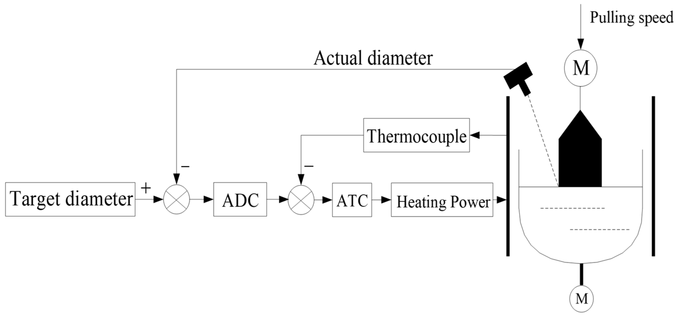
Figure 1. Simplified control structure for CZ silicon single-crystal diameter growth control. Target diameter is the reference/setpoint; actual diameter and thermocouple temperature are measured feedback variables; pulling speed and heating power are manipulated variables; ADC and ATC denote control blocks; disturbances (not explicitly shown) mainly represent unmeasured thermal–fluid perturbations inside the furnace.
Processes 14 01153 g001
Figure 2. The MIC correlation matrix for the top 15 features.
Processes 14 01153 g002
Figure 3. Structure of a standard temporal convolutional layer with full receptive field connections.
Processes 14 01153 g003
Figure 4. Dilated temporal convolutional layers with increasing dilation factors (d = 1, 2, 4).
Processes 14 01153 g004
Figure 5. Residual block structure of the temporal convolutional network (TCN).
Processes 14 01153 g005
Figure 6. Internal computational structure of a Long Short-Term Memory (LSTM) unit.
Processes 14 01153 g006
Figure 7. Overall architecture of the proposed TCN-LSTM hybrid model.
Processes 14 01153 g007
Figure 8. TCN-LSTM model (no time delay, no history) prediction results (comparison of actual and predicted values).
Processes 14 01153 g008
Figure 9. Prediction results of TCN-LSTM model (no time delay, including history) (comparison of actual and predicted values).
Processes 14 01153 g009
Figure 10. Prediction results of TCN-LSTM model (with time delay, no history) (comparison of actual and predicted values).
Processes 14 01153 g010
Figure 11. Prediction results of TCN-LSTM model (with time delay and historical data) (comparison of actual and predicted values).
Processes 14 01153 g011
Figure 12. Comparison of the TCN-LSTM prediction curves under the four input configurations.
Processes 14 01153 g012
Figure 13. Overall comparison of prediction results of the three models under four settings (different colors correspond to different models and settings, solid lines represent the true values).
Processes 14 01153 g013
Figure 14. Convergence process of hyperparameter optimization (GWO) of TCN-LSTM model.
Processes 14 01153 g014
Figure 15. Prediction results of the GWO-optimized TCN-LSTM model (comparison between actual and predicted values).
Processes 14 01153 g015
Figure 16. Bar chart of the importance of each input feature SHAP in the TCN-LSTM model (after GWO).
Processes 14 01153 g016
Figure 17. SHAP summary (beeswarm) plot of the GWO-optimized TCN-LSTM model; each point represents the feature contribution of one sample.
Processes 14 01153 g017
Table 1. Explanation of process variables and symbols.
No.Variable Name
1Average_growth_rate
2Crucible_lift_rate
3Crystal_pull_rate
4Crystal_length
5Crystal_weight
6Crystal_rotation_speed
7Heater_temp
8Main_heater_voltage
9Main_heater_power
10Main_heater_current
11Sub_heater_power
12Sub_heater_current
13Main_heater_resistance
14Sub_heater_voltage
15Sub_heater_resistance
Table 2. The metrics of all models under different configurations.
Model & ConfigurationMSERMSEMAER2
TCN-LSTM, nolag-noY0.027940.167160.142720.68585
TCN-LSTM, nolag-withY0.003900.062420.045330.94587
TCN-LSTM, withlag-noY0.020570.143410.121590.70594
TCN-LSTM, withlag-withY0.002590.050870.039490.96982
TCN-LSTM, GWO0.002390.048940.036510.97207
TCN, nolag-noY0.029870.172830.148770.66416
TCN, nolag-withY0.016130.127010.097720.81864
TCN, withlag-noY0.020660.143750.120750.75904
TCN, withlag-withY0.012760.112940.087910.85124
LSTM, nolag-noY0.042410.205940.186170.52317
LSTM, nolag-withY0.012410.111400.086840.86383
LSTM, withlag-noY0.037790.194410.152570.55927
LSTM, withlag-withY0.003440.058660.047260.96078
Disclaimer/Publisher’s Note: The statements, opinions and data contained in all publications are solely those of the individual author(s) and contributor(s) and not of MDPI and/or the editor(s). MDPI and/or the editor(s) disclaim responsibility for any injury to people or property resulting from any ideas, methods, instructions or products referred to in the content.