1. Introduction
Seismic exploration is highly important for the prediction and identification of oil and gas reservoirs. Seismic data can be used to determine the structural characteristics of underground media and information about oil- and gas-bearing strata interfaces. In reservoir prediction, seismic wave impedance inversion plays a key role in identifying oil and gas reservoirs. The wave impedance inversion technique was first proposed by Kuster (1974) [
1], and wave impedance inversion can be divided into prestack and poststack inversions. Prestack wave impedance inversion involves prestack wave equation inversion [
2,
3,
4] and elastic impedance inversion [
5,
6]. This method requires more geologic data, involves a more complex inversion process, and demands greater computational effort; however, it provides greater inversion accuracy and yields abundant elastic parameters of underground media, making it an important direction in the development of seismic inversion. Nonetheless, poststack inversion remains widely used in actual production because of its relatively simple algorithm, low influence of noise and ease of implementation [
7]. However, owing to the limitations of seismic data, noise interference and approximation in forward modelling, the seismic inversion problem remains incompletely addressed. Even a small amount of noise in seismic data can cause instability in the inversion process, and the seismic data remain nonunique [
8].
During field seismic data acquisition, collected records are often contaminated by noise interference because of multiple factors, including construction environments and equipment conditions. These disturbances not only cause signal confusion but also severely degrade continuous effective signals, directly affecting the signal-to-noise ratio of seismic data and the quality of subsequent processing and interpretation. From the perspective of spatial coherence, seismic noise can be broadly categorized into two types: random noise and regular noise. During seismic exploration, signals captured by surface-mounted sensors are often contaminated by random noise, which adversely affects subsequent processing performance. Consequently, removing random noise from noisy data is a critical step. This noise exhibits random characteristics, with a broad frequency distribution and no fixed dominant frequency or apparent velocity. Common random noise suppression methods typically leverage the sparsity of signals in seismic data. By mapping seismic data into the transform domain, these methods can fully utilize the characteristics of signals within this domain to achieve signal reconstruction, thereby removing random noise. Sparse transform-based approaches enable the effective separation of signals and noise in the transform domain, where signals exhibit sparsity while noise does not. Therefore, only the soft threshold operator is needed to set the coefficients in the transformed sparse domain, and the sparse coefficients are finally converted to the time domain to reconstruct the clear signal. For example, the Fourier transform [
9], the Radon transform [
10,
11], the wavelet transform [
12,
13,
14], the seislet transform [
15,
16], the dreamlet transform [
17], the curvelet transform [
18,
19] and the contourlet transform [
20] can be used to characterize seismic data.
Compared with random noise, regular noise has a greater effect on the quality of seismic data processing. Among the various types of noise, surface waves are among the most prevalent and widespread regular noise sources. In complex terrain, they exhibit intense energy, intricate spatial trajectories, and characteristics overlapping with valid signals, sometimes even distorting or drowning out the valid signals. Although multiple suppression methods have been developed, they typically require regular interference to follow specific mathematical curves with spatially stable energy and frequency. However, real-world interference often fails to meet these mathematical criteria, resulting in nonstationary variations in trajectory, energy, and frequency across space. Consequently, these methods not only retain substantial noise energy but also cause significant damage to seismic signals during implementation.
In recent years, the application of machine learning to the interpretation and processing of seismic data has attracted widespread attention, such as in fault segmentation [
21] and velocity model construction [
22]. Using machine learning, we can extract valuable insights from data by learning multilevel abstract representations [
23]. To date, label-based machine learning methods have been successfully applied to suppress noise in seismic data [
24]. These methods can be divided into two categories based on the generation strategy of the labels. In the first category, the labels are derived from the outputs of existing denoising methods, and the neural network is trained using these labels [
25]. However, some problems still exist in practical applications, such as random noise in seismic data after denoising, which can lead to inaccurate labels. In the second type, labels are generated by creating synthetic data [
26]. However, creating a training set that closely resembles actual noise is quite difficult. Consequently, the extracted features may not fully match the actual seismic records received, which could impair the denoising performance of the neural network. Moreover, while label-based machine learning approaches can produce effective denoising results, generating large-scale and diverse training datasets remains a labour-intensive process. The process of noise removal is complicated, and the effect is not ideal. Therefore, we aimed to discover if there is a seismic wave detection method that is less sensitive to noise and easier to invert.
2. Theoretical Research
From a study of the relevant literature [
27,
28,
29,
30,
31,
32], we know that the Earth’s surface itself vibrates continuously with a very small amplitude (from 10
−5 to 10
−3 cm), and these are called microtremor. Microtremor occur at all times and locations, constituting regular noise in reflection-based seismic exploration. Influenced by both regular and random noise signals, the morphology and amplitude of micromotion vary with spatial and temporal changes. However, within specific spatiotemporal domains, it exhibits stable statistical properties, allowing description through the theory of stationary stochastic processes. Micromotion exploration technology fundamentally relies on the following theory: the frequency curves of surface waves are extracted from micromotion signals and then inverted to determine the velocity structure of underground shear waves. Currently, the F-K method and autocorrelation method are the primary techniques for measuring surface wave dispersion information using micromotion signals.
The propagation speed of microtremor signals varies across different geological formations. In looser strata, signal propagation tends to be slower, with significant energy loss occurring during transmission through such porous layers. In areas with thick sedimentary deposits, microtremor signals exhibit noticeable amplitude decreases and frequency shifts after propagation. Conversely, in hard rock formations, signals travel faster with minimal energy loss. When underground rock layers exist, microtremor signals can maintain their original characteristics and propagate relatively intact over long distances. The presence of faults in subsurface formations causes reflection and refraction phenomena. Faults act as “cracks” in geological structures: while some signals pass directly through these breaks, others are reflected back, resulting in complex signals being received by detection instruments. In regions with extensive fault networks, multiple overlapping signals may appear in the data, as reflected waves mix with the original propagation signals. The stratified structure of strata also affects microtectonic signals, with interfaces between different layers acting as “barriers” that cause signal refraction during passage.
The instruments and equipment needed for the construction of micromotion exploration technology are relatively simple and easy to operate. Micromotion exploration technology requires no more than three seismometers for field operations. When seven seismometers are arranged in a double concentric equilateral triangle configuration, underground shear wave velocity distributions at depths of hundreds of metres can be mapped within 3–5 days. This method has low environmental requirements, making it particularly suitable for densely populated urban areas. Unlike conventional reflection-based exploration techniques, micromotion exploration employs natural “noise” as its signal source. In busy city environments, vehicle movement not only does not interfere with the surveys but also provides abundant signal sources. As a passive exploration method, it minimally impacts surrounding environments, making it ideal for regions with strict environmental protection standards. This technology delivers highly reliable results with exceptional resolution, and when combined with borehole drilling, it enables the creation of 2D and 3D subsurface structural models. Measurements from micromotion exploration show remarkable consistency with P-S logging results, demonstrating exceptional reliability. With advantages such as simplicity, cost-effectiveness, and environmental friendliness, this method is particularly advantageous for exploring mining structures and petroleum resources.
In urban shallow geotechnical engineering, micro-motion array detection provides critical geophysical parameters such as S-wave velocity and soil layer thickness [
33]. This technology enables sediment layer thickness measurement [
34], playing a vital role in site stability assessment and non-destructive quality inspection. Tian et al. [
35] developed a mini-array micro-motion detection method that effectively identifies varying weathering degrees of rock masses, offering detailed shallow geological structures. Meanwhile, Tian Baoqing et al. [
36] conducted cross-disciplinary research integrating geophysical parameters from micro-motion detection with refined geothermal resource reserve evaluation and petrological parameters. By utilizing thickness parameters of lithologic layers obtained through mini-array micro-motion detection, they improved the USGS-based geothermal resource reserve evaluation method, significantly enhancing assessment accuracy and identifying optimal development zones. In cross-disciplinary studies, they proposed a method to predict thermal conductivity using geophysical parameters, establishing empirical relationships between S-wave velocity, density, and thermal conductivity. This approach allows prediction of thermal conductivity trends in areas underserved by thermal response tests, extending from point to area.
The single-unit micro-motion method utilizes micro-motion signals recorded by three-component stations for underground geological structure detection, primarily referring to the H/V spectral ratio method. This method, based on three-component micro-motion signals, has been widely adopted due to its simplicity, practicality, and information-rich nature, and has now evolved into one of the most common techniques. The H/V spectral ratio method was first proposed by Nogoshi and Igarashi and later popularized by Nakamura. The method calculates the Fourier spectra of horizontal and vertical components, then computes their ratio to obtain the H/V spectral ratio curve. The spectral ratio curve can identify peak frequencies, which exhibit a strong correlation with site natural frequencies. For the same site, peak frequencies generally remain stable and exhibit an exponential relationship with sediment layer thickness. Additionally, the amplitude of the spectral ratio curve serves as a reference for determining the amplification coefficient of sedimentary sites [
37].
Since the introduction of the micro-motion H/V spectral ratio method by Nakamura, numerous researchers have conducted experiments across various countries and regions [
38,
39,
40]. In Europe, researchers from multiple countries have implemented the SESAME (Site EffectS assessment using AMbient Excitations) project and published related research reports. Similar to surface wave dispersion curves, spectral ratio curves also reflect underground structures. Arai and Tokimatsu [
41] pioneered the study of spectral ratio curve inversion. In China, Chen Qifu et al. [
42] used the spectral ratio method to detect seismic responses in Beijing’s urban area and estimate sediment thickness. Wang Weijun et al. [
43] combined the spectral ratio method with the F-K method to analyze shallow velocity structures in Beijing, determining the lower limits of the city’s peak frequency and amplification coefficient.
3. Microtremor Test
This study examines an engineering case to demonstrate the application value of micromotion detection in shallow natural gas reservoir structures. The experimental site is located in sedimentary rocks with a 5–15° monocline structure, featuring a rice field with long-term water-soluble natural gas seepage. Frequent observations of massive gas bubbles emerging from the rice fields indicate substantial underground gas reservoirs and demonstrate the presence of continuous gas movement. To investigate shallow gas reservoir structures, micromotion surveys were conducted, focusing on the application of micromotion detection in shallow gas reservoir geology. Simultaneously, integrated drilling and electrical logging comparisons were performed to verify the flow paths of natural gas migration.
Micromotion observations provide comprehensive data, including soil layer locations and geological structures. Through spectral analysis, the frequency characteristics of microseismic signals can be extracted to reveal the dynamic properties of a measured area. By analyzing the dispersion of the recorded signals and applying the fast Fourier transform (FFT) method, the dominant surface frequency can be estimated. The linear distribution of gas emissions on the ground suggests the presence of a near-north–south trending fault beneath the strata. The design of the initial wiring scheme is based on the preliminary geological survey findings. The initial field micromotion detection layout is shown in
Figure 1 (Scale 1:1000).
During data acquisition, a 23-metre seismic line with 1-metre spacing is used between receivers. The measurement and data collection equipment employs a portable seismometer (16-bit resolution) with a detection frequency range of 0 Hz to 70 Hz. The primary measurement parameters of the microseismic equipment are listed in
Table 1. During field surveys, human disturbances should be minimized, and the site should be as flat as possible. Short-term microseismic horizontal and vertical component records are obtained using a triaxial high-sensitivity seismometer (natural period of 1 s). The equipment measures two horizontal components (EW and NS) and one vertical component (UD) of microseismic events. Designed with a sampling rate of 100 Hz, the system records continuously for 5 min, resulting in the accumulation of a total of 30,000 data points. Two measurement lines are employed: Line A has 5 monitoring points, whereas Line B has 7 monitoring points spaced 10 m apart.
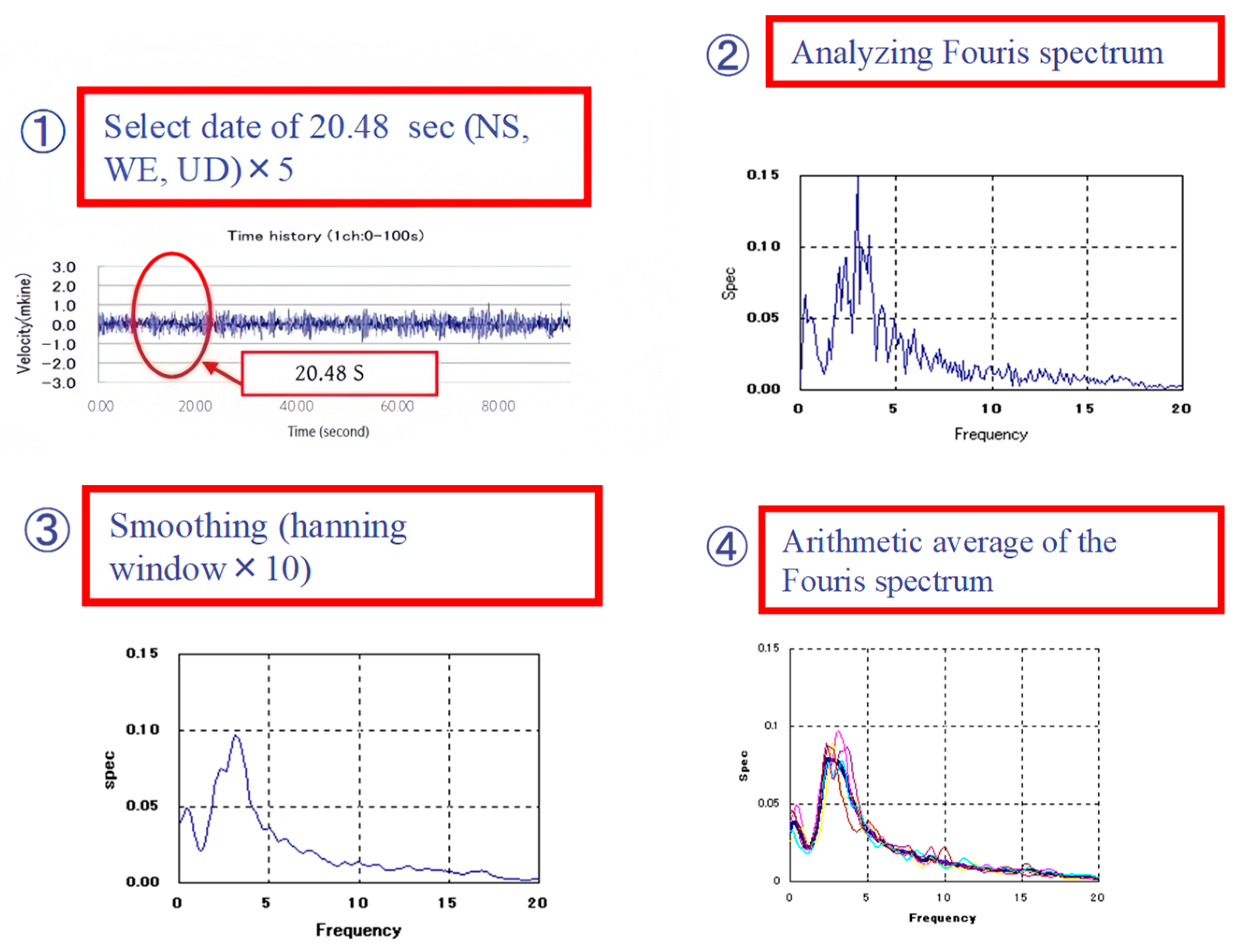
The survey line is perpendicular to the fault, with the measurement workflow illustrated in
Figure 2. The microseismic data are analyzed using fast Fourier transform (FFT). By examining the signal spectrum, we can identify the frequency characteristics of microseismic events, which can aid in the investigation of the dynamic properties of the structural features in the measured area. After the observation signals are processed with FFT, five low-noise cycles of 20.48 s data are selected from the microseismic measurements for analysis. This involves calculating the Fourier amplitude spectrum, spectral ratio, and relative amplitude change.
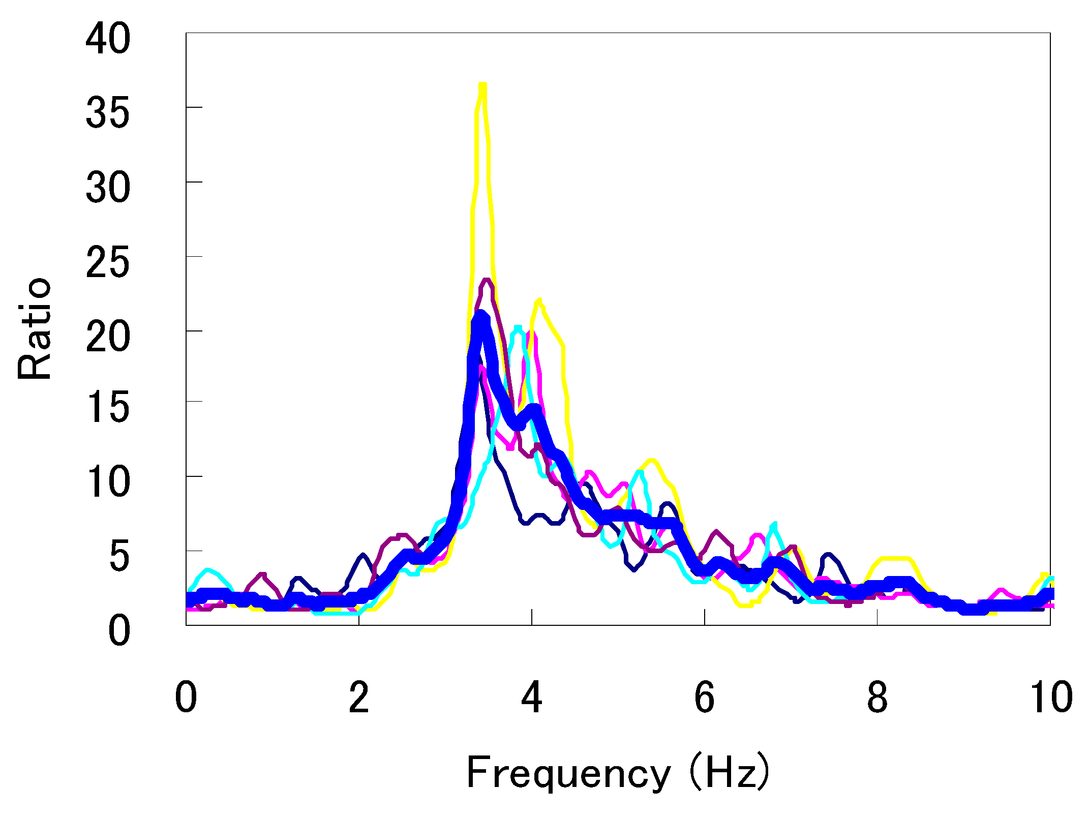
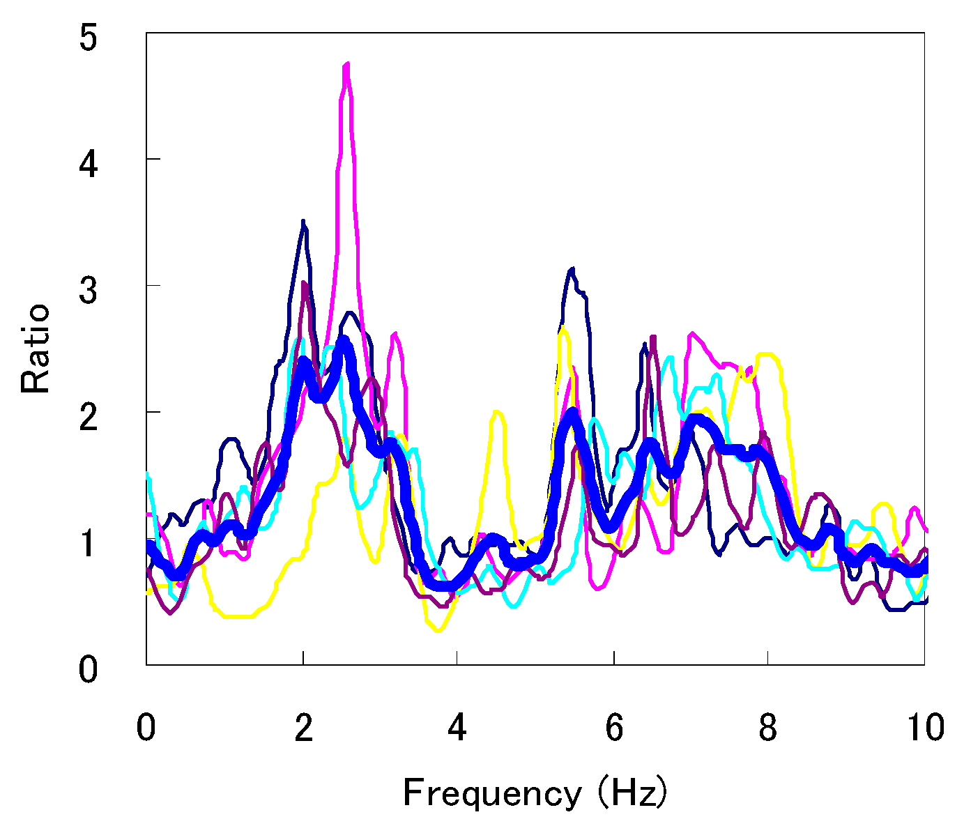
The primary objective of ground station dominant frequency determination is to obtain the microseismic amplitude and dominant frequency. In the Nakamura method, three Fourier spectra are acquired. By dividing the horizontal components (north–south and east–west) by the vertical component (up–down), the ground transfer function and dominant frequency are derived. This method is characterized by simplicity and rapid computational speed. The H/V analysis results are shown in
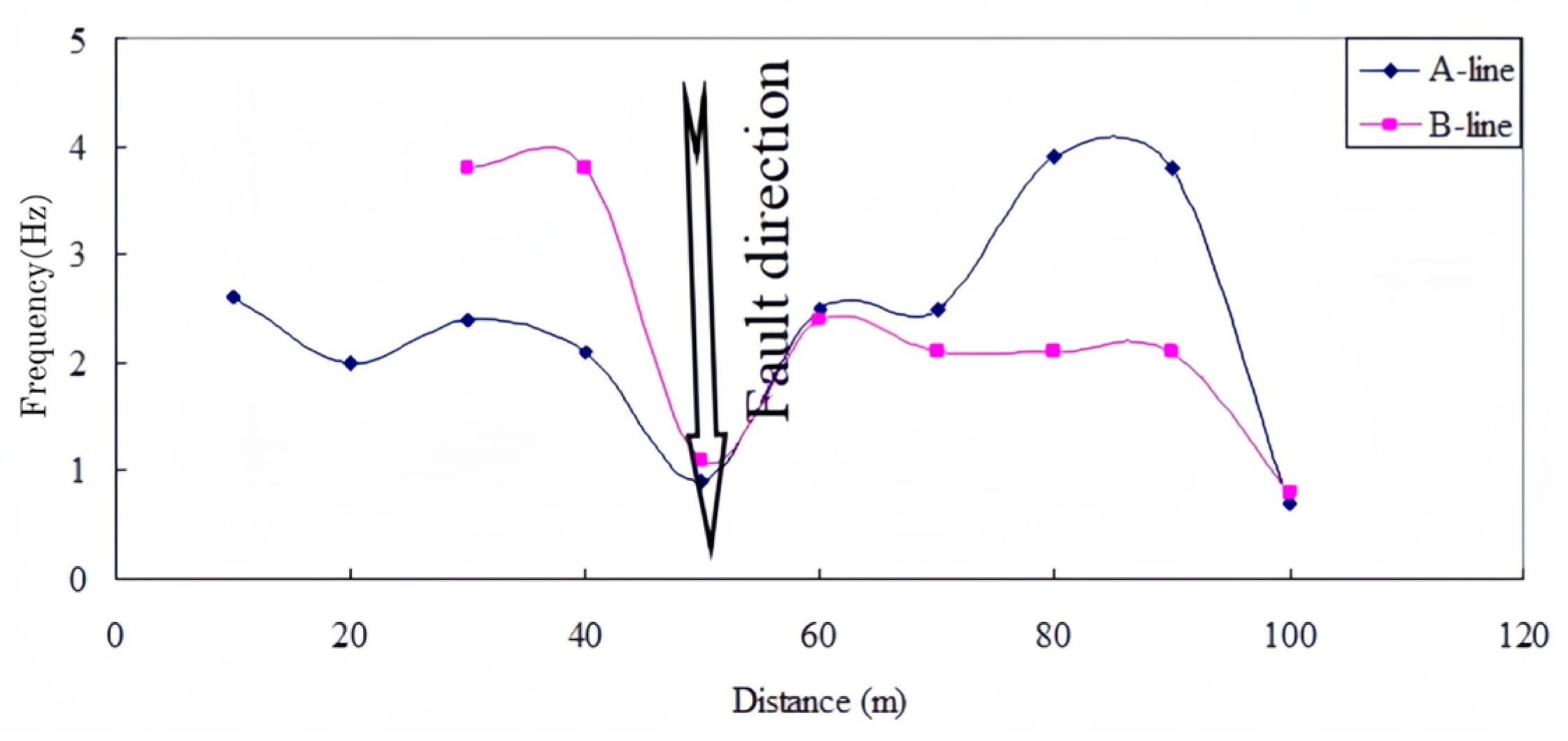
Figure 3, where the H/V components exhibit distinct peak amplitudes, indicating fault reflections. The dominant frequency distribution along the observation direction is shown in
Figure 4. After the other possible error is eliminated, the significant peak amplitude indicates the existence of fault.
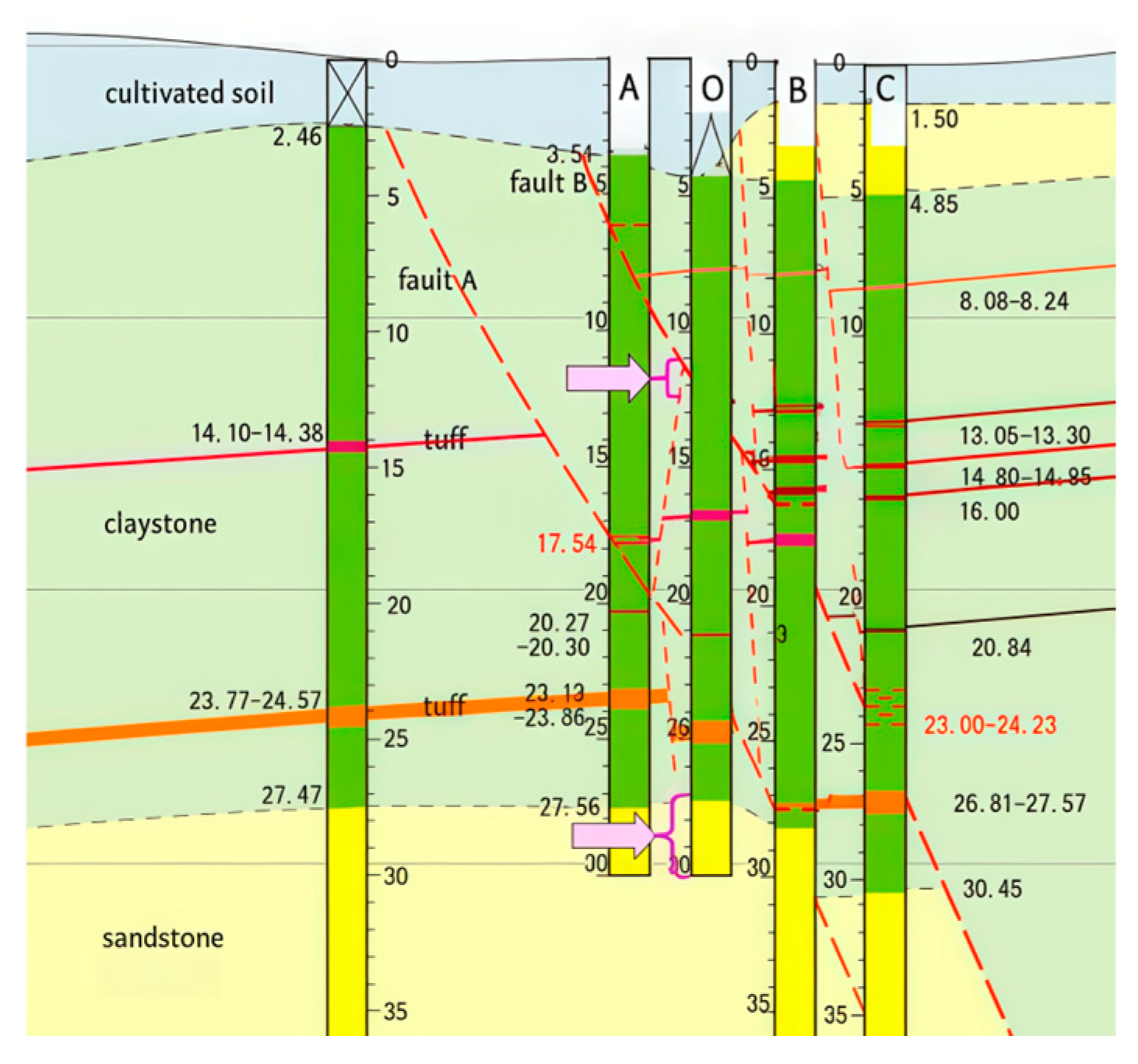
To verify the accuracy of micromotion detection, a drilling survey was conducted in the test area. The borehole data indicate that the strata are primarily composed of alternating layers of sandstone and claystone. The surveyed area features two north–south-trending normal faults, with the eastern side of the faults constituting the upper plate. The northern side of this upper plate has a subsiding structure. Approximately three metres below the cultivated soil lies a layer of claystone interspersed with tens of centimetres of tuff rock, and beneath this layer lies sandstone strata. The stratigraphic and fault distributions revealed by the boreholes are shown in
Figure 5.
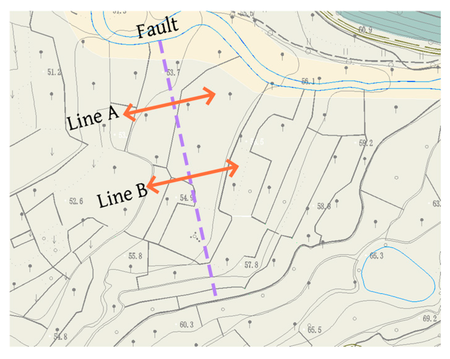
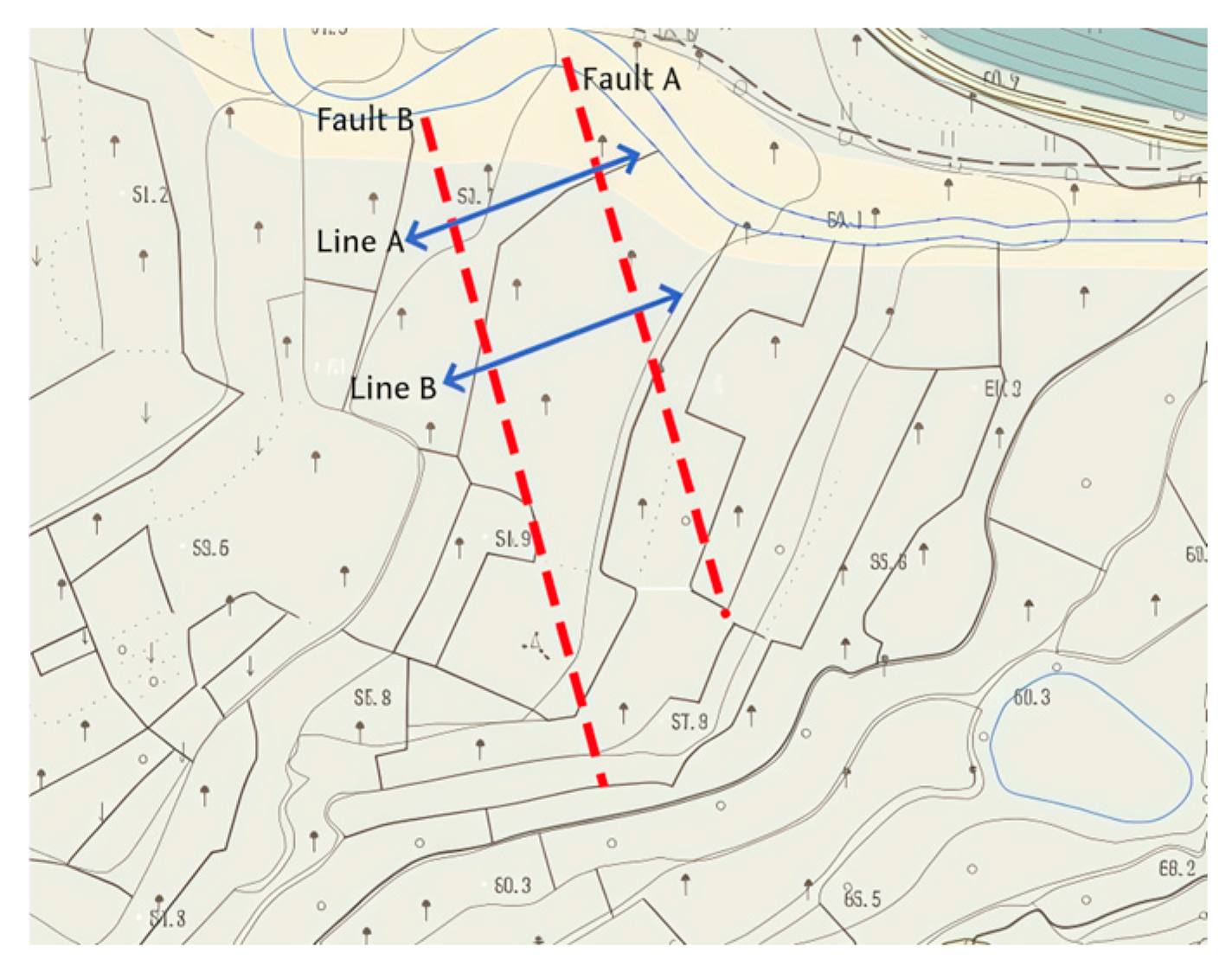
Field drilling revealed two nearly parallel faults within the strata. The initial micromotion detection failed to fully capture the fault distribution because of inadequate wireline placement. To evaluate the precision of micromotion detection, two new micromotion lines were established perpendicular to the existing faults, with Line A and Line B positioned as shown in
Figure 6.
The results of the analysis of the second micromotion detection test are presented in
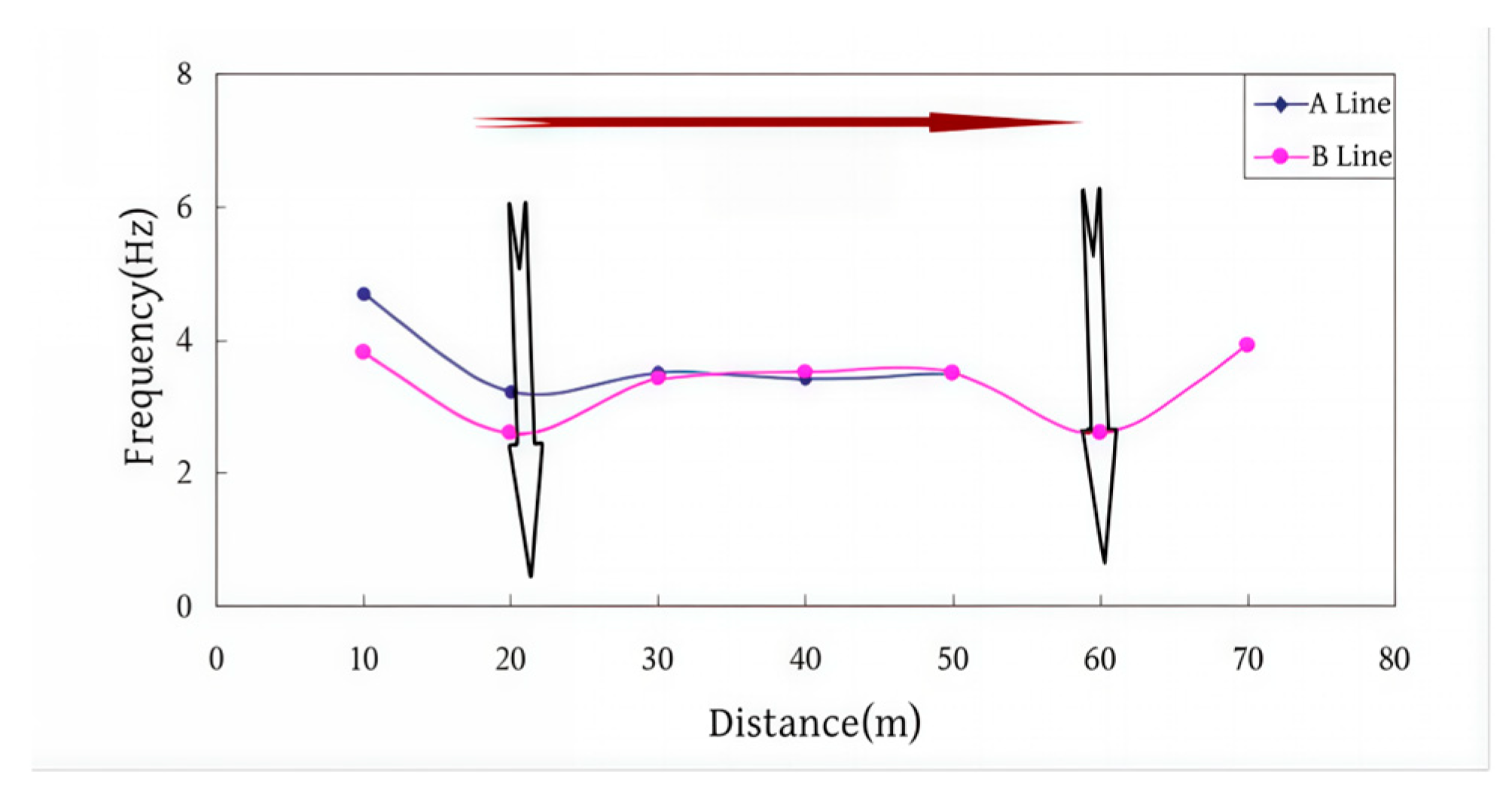
Figure 7. H/V analysis reveals two distinct peak amplitudes that correspond to the fault locations in the formation. The dominant frequency distribution along the observation direction is shown in
Figure 8. The frequency distribution at the fault observation points exhibits an inverted response pattern, which closely matches the strike trend of the faults identified through drilling.
4. Electrical Geophysical Prospecting
Micromotion detection data can be used to identify fault locations in shallow gas reservoir structures; however, understanding natural gas flow paths requires combining it with other geophysical methods. According to the basic principles of electrical geophysical exploration, groundwater resistivity typically ranges from tens to hundreds of ohms, whereas brine has a resistivity of only approximately 0.3 ohms—a difference of hundreds of times. When highly saline brine is directly injected into boreholes, the resistivity of rock layers in the brine-soaked zone decreases. By measuring resistivity changes before and after brine injection, researchers can easily identify areas with reduced resistivity. The analysis of resistivity variations in surrounding observation wells is useful for determining water infiltration directions, revealing flow paths and directions. Simultaneously, studying spatial distribution changes in rock resistivity enables the visualization of geological structures.
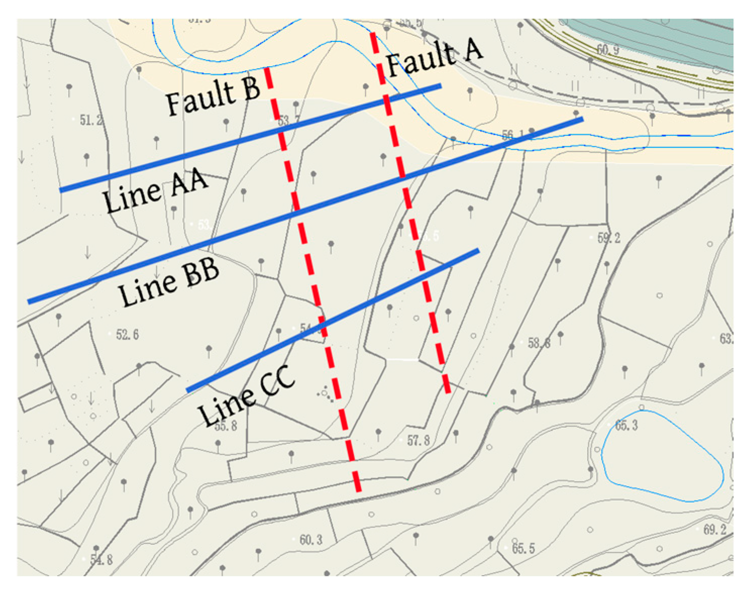
To determine the flow path of underground natural gas, electrical geophysical exploration was conducted. First, a borehole was drilled at the fault centre, after which brine was injected. By analyzing changes in subsurface rock resistivity through electrical equipment, the underground conditions were visualized to infer the fluid flow direction and route, thereby revealing the natural gas seepage path. Three survey lines were arranged near the rice fields on the north side of the test site in an east–west direction, as shown in
Figure 9. Survey lines AA (430 m), BB (595 m), and CC (295 m).
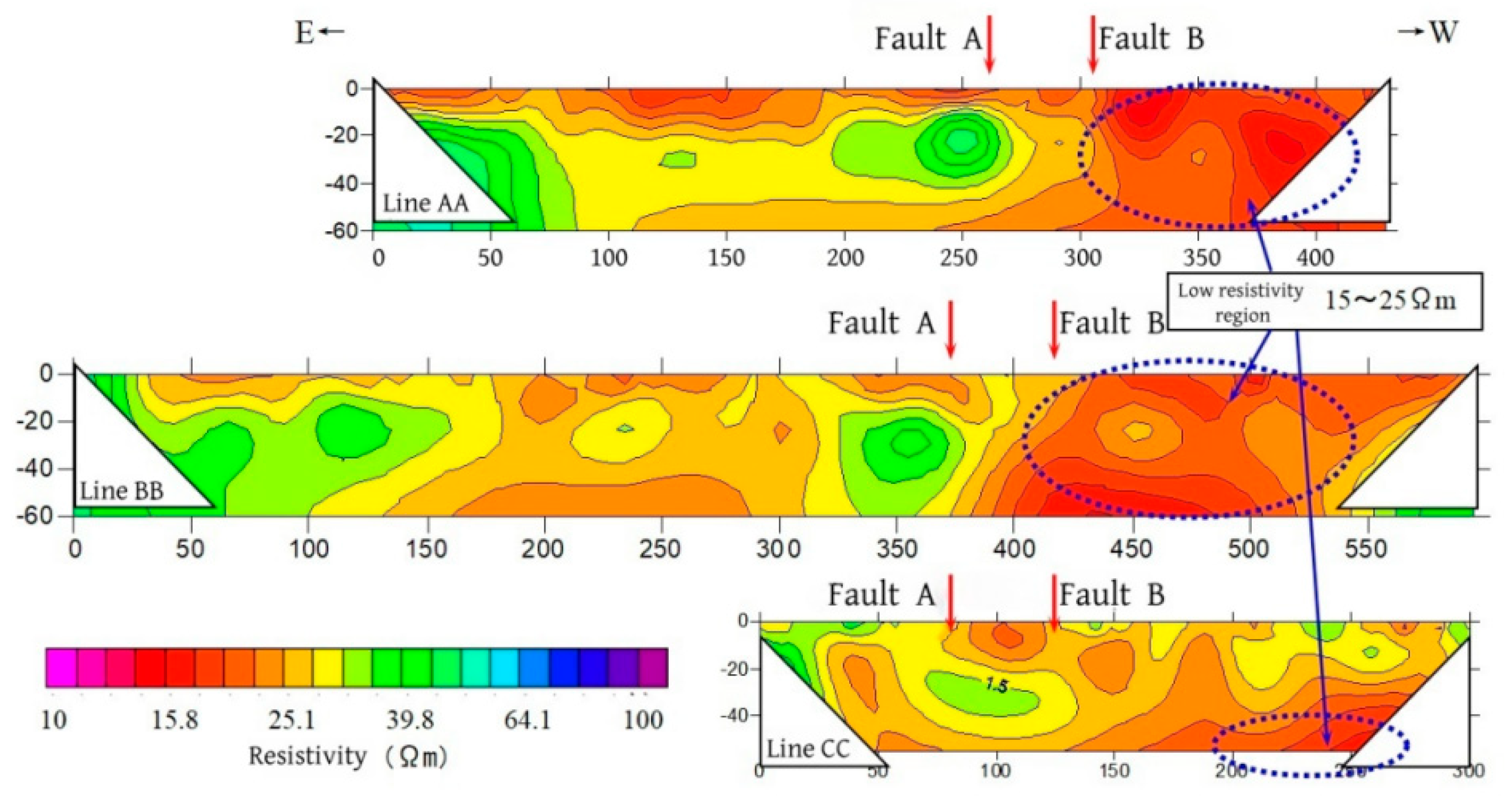
The resistivity profiles of the three survey lines are shown in
Figure 10. The test data indicate that the tested area has resistivity values ranging from 15 to 40 ohms. Drilling surveys in the experimental zone reveal alternating layers of sandstone and claystone as the predominant geological formation. Notably, low-resistivity zones are observed west of survey lines AA and BB, which are likely due to the presence of claystone sedimentary layers and higher water content in the strata.
Table 2 presents the resistivity measurements of the borehole core samples. The resistivity of the sandstone ranges from 81 to 82 Ω·m, whereas that of the clayey mudstone ranges from 18 to 28 Ω·m. The samples were prepared by grinding the rock cores into cylindrical shapes, immersing them in distilled water, and measuring the resistivity after vacuum degassing and saturation. The higher resistivity of sandstone and the slightly lower resistivity of claystone align with the borehole survey results recorded on the CC survey line.
Four boreholes were set up in the field; the depth of water injection hole O was 50 m, and the depths of the other three observation holes ABC were 30~80 m. Salt water was injected into the water injection hole, and the change in resistivity was observed at the other three boreholes; the distribution of the boreholes is shown in
Figure 5.
Brine was injected into the upper section of the clay layer at −11.3~−12.3 m and into the lower section of the sandstone at −24 to −30 m. The electrical conductivity of the brine solution ranged from 53 to 54 mS/cm. The total injection volume was 2.21 m3 for the upper section and 2.98 m3 for the lower section. Seven hours were required to inject water into the upper section. The resistivity was measured once before water injection, 5 times during water injection, and 2 times after water injection, for a total of 8 measurements. Water was injected into the lower section twice. The resistivity was measured once before water injection, 6 times during water injection, and once after water injection, a total of 8 times.
Three observation holes were drilled and fitted with electrodes using the same method, and continuous analysis was performed during water injection. The electrode array consisted of 30 multiconnected electrode arrays spaced 50 cm apart, which could be tested at a distance of 14.5 m at one go. The visual resistivity calculation formula for electrode deployment in a hole is as follows:
where V is the test voltage, I is the current, a is the electrode spacing, and n is the electrode isolation factor. The apparent resistivity is the equivalent resistivity measured by a specific electrode device and converted. This parameter is not the true resistivity of a single rock but a comprehensive indicator reflecting the electrical characteristics of various rocks within the detection range.
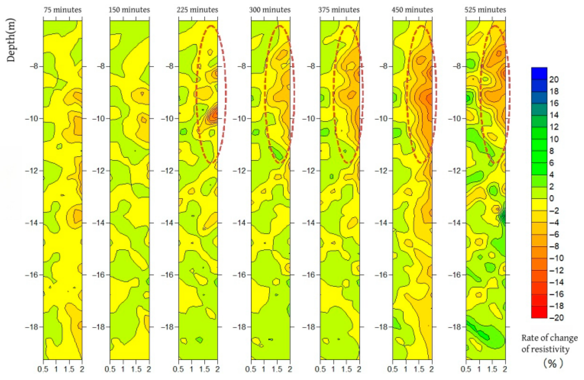
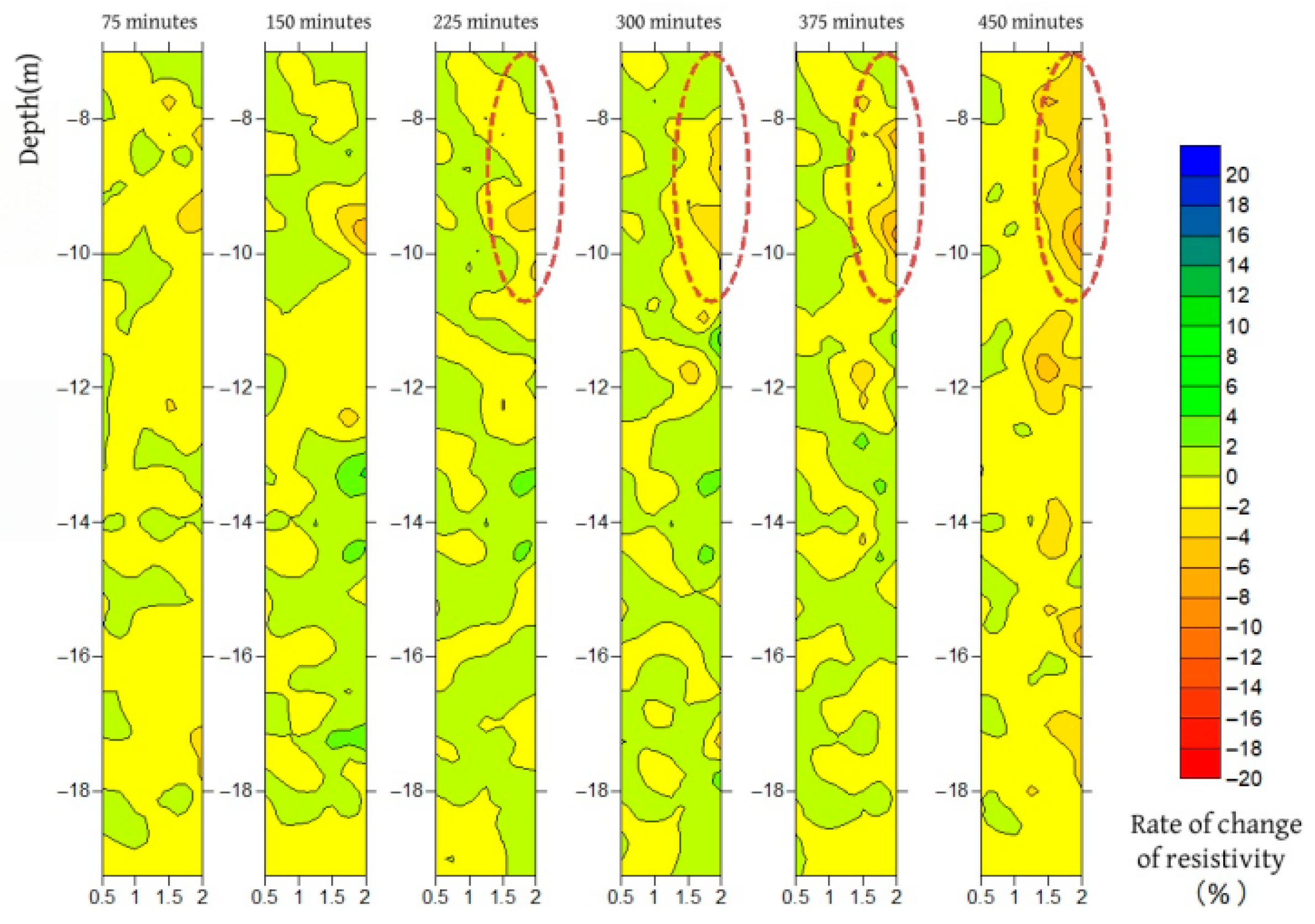
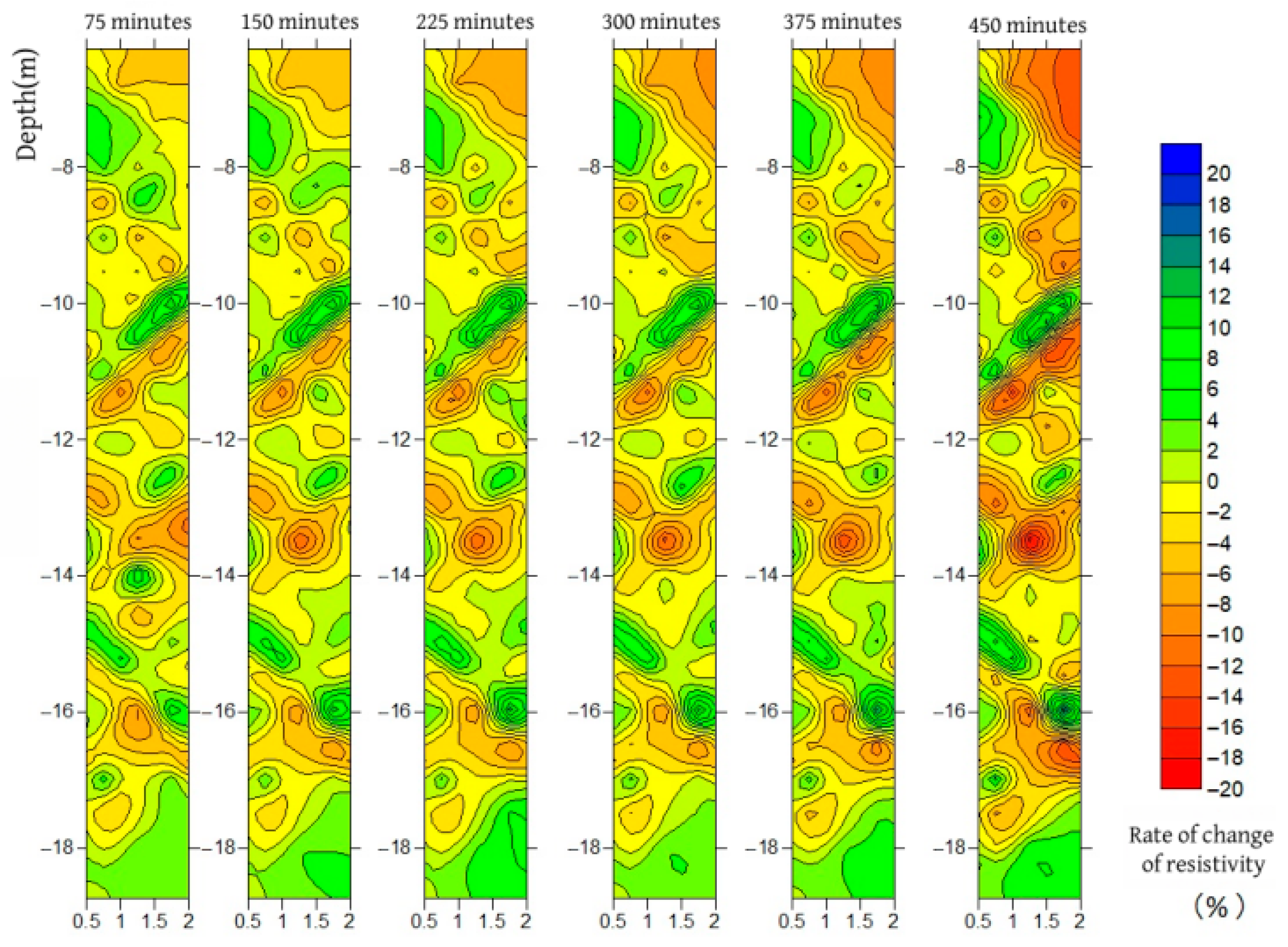
The rate of change in resistivity was calculated using the data for the resistivity before and after the injection of brine solution, and the effect of the brine solution on the measured value was confirmed. In
Figure 11,
Figure 12 and
Figure 13, the horizontal axis indicates the depth from the borehole opening and the electrode positions, whereas the vertical axis shows the apparent depth at the centre of the electrode array. The variation rate distribution of the apparent resistivity measured in the upper interval is illustrated in
Figure 11,
Figure 12 and
Figure 13.
In the depth range from 2 m to −6 to −11 m in observation hole A, the apparent resistivity gradually decreased over time, with the maximum change being approximately 10%, as indicated by the circle in the figure. The rate of resistivity change in observation hole B was more complex than that in the initial stage, but it also decreased over time. The maximum decrease in resistivity was −6% in observation hole C at −7~−10 m.
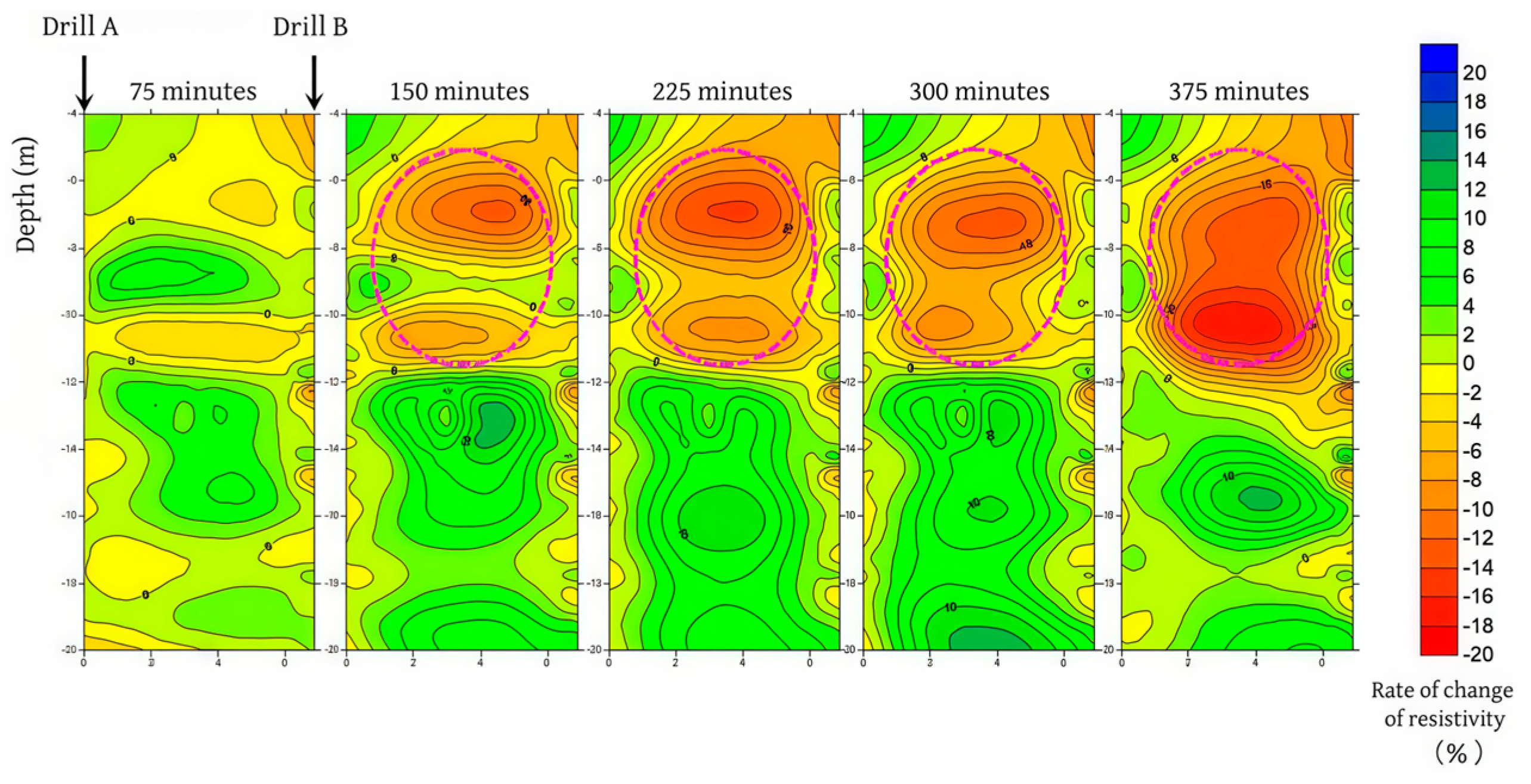
The change in resistivity between observation wells A and B is shown in
Figure 14. On the basis of the initial resistivity profile, a two-dimensional analytical cross-section of the change in resistivity is derived. The resistivity decreases over time in the range of −6 to −12 m, with a maximum decrease of −16%, as indicated by the circled area in the figure. Based on the above study, it can be concluded that the brine injected into the fractured portion of the injection well (−11.3~−12.3 m) mainly seeps into the fractured zone on the north side of the lower part of the north-side fracture, which is more inclined than observation well A (westwards).
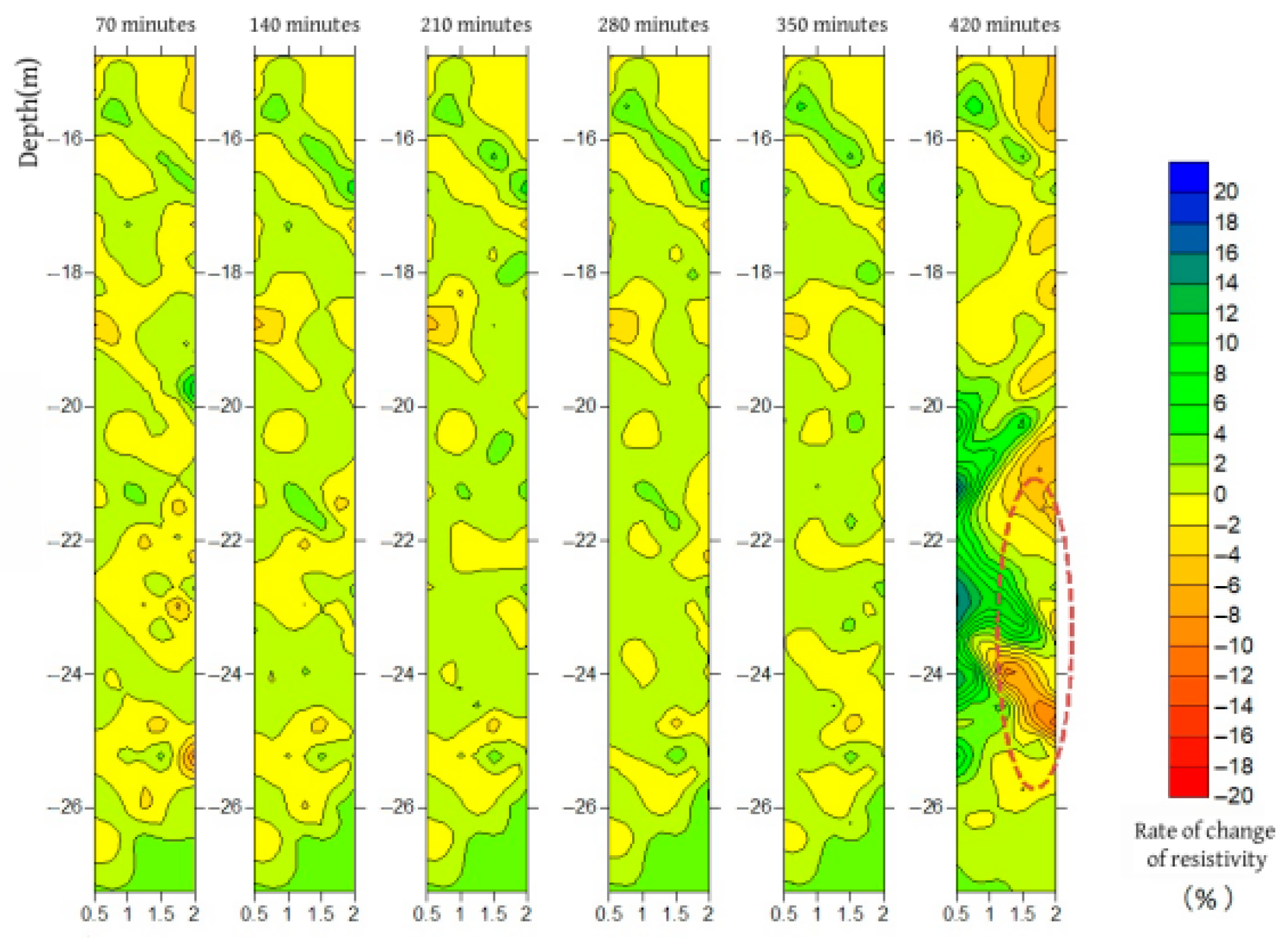
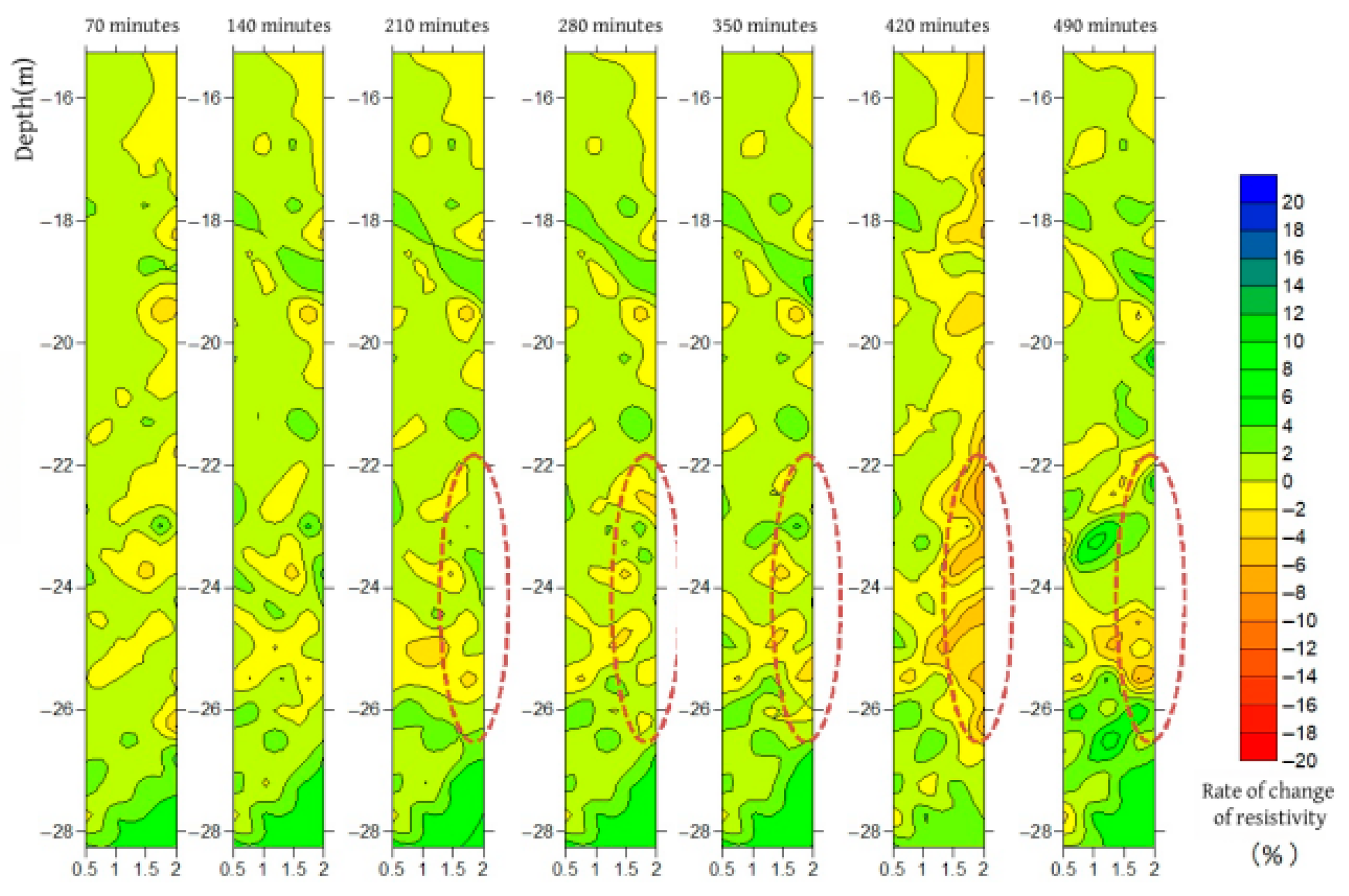
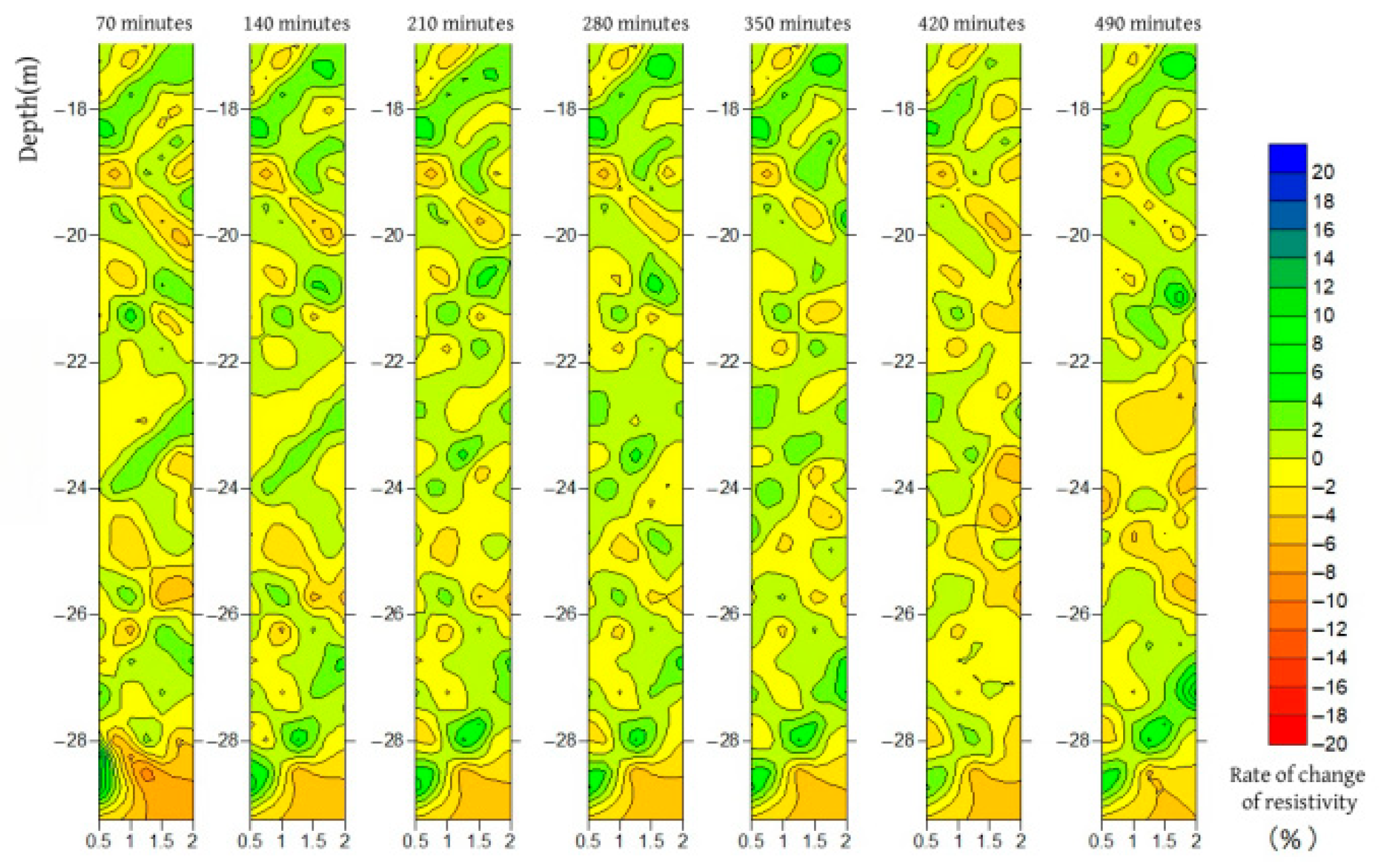
The distribution of the apparent resistivity measured in the lower interval is shown in
Figure 15,
Figure 16 and
Figure 17. A maximum change of −6% in the −22 to −26 m interval was recorded for observation well A, whereas a peak change of −8% in the −21 to −25 m range was recorded for observation well B. Within the apparent depth range of 1.5 to 2 m, the apparent resistivity tended to decrease over time, as indicated by the circled areas in the figure. Observation well C demonstrated minimal resistivity variation over time. The resistivity inversion maps reveal that the brine injected from the lower sandstone layer primarily permeated in a northwesterly direction.
5. Conclusions
Minor noise in seismic data can lead to significant errors during inversion processes, with both random and regular noise substantially affecting data processing quality. Although machine learning methods can produce effective denoising results, the denoising process remains complex and often yields suboptimal outcomes. Micromotion exploration technology, which is grounded in the theory of stationary random processes, involves extracting the frequency curves of surface waves from micromotion signals. Through the inversion of these curves, the velocity structure of underground shear waves can be accurately determined. Microseismic exploration technology is less affected by random noise and regular noise, even enabling data analysis for shallow gas reservoir structure interpretation. In practical applications, while fault detection is effective for gas reservoir identification, the limited richness of data often restricts deeper reservoir characterization. Electrical geophysical methods are excellent for visualizing geological formations, as variations in rock formation resistivity directly reveal water flow paths and natural gas migration routes, offering distinct advantages in shallow reservoir evaluation. For comprehensive exploration, microseismic and electrical geophysical techniques should be integrated to leverage their complementary strengths to increase structural investigation operational efficiency.
Author Contributions
Conceptualization, F.Z.; methodology, F.Z.; software, F.Z.; validation, F.Z., M.Z. and J.S.; formal analysis, F.Z.; investigation, F.Z.; resources, F.Z.; data curation, F.Z.; writing—original draft preparation, F.Z.; writing—review and editing, F.Z.; visualization, F.Z.; supervision, F.Z.; project administration, F.Z.; funding acquisition, F.Z. All authors have read and agreed to the published version of the manuscript.
Funding
This research received no external funding.
Data Availability Statement
The original contributions presented in this study are included in the article. Further inquiries can be directed to the corresponding author.
Conflicts of Interest
The authors declare no conflicts of interest.
References
- Kuster, G.T.; Toksöz, M.N. Velocity and attenuation of seismic waves in two-phase media, Part 1, Theoretical formulations. Geophysics 1974, 39, 587–606. [Google Scholar] [CrossRef]
- Greenberg, M.L.; Castagna, J.P. Shear-wave velocity estimation in porous rocks: Theoretical formulation, preliminary verification and applications. Geophys. Prospect. 1992, 40, 195–209. [Google Scholar] [CrossRef]
- Xu, S.; Payne, M.A. Modeling elastic properties in carbonate rocks. Lead. Edge 2009, 28, 66–74. [Google Scholar] [CrossRef]
- Sun, S.Z.; Wang, H.Y.; Liu, Z.S.; Li, Y.W. The theory and application of DEM-Gassmann rock physics model for complex carbonate reservoirs. Lead. Edge 2012, 31, 152–158. [Google Scholar] [CrossRef]
- Eskandari, H.; Rezaee, M.; Mohammadnia, M. Application of multiple regression and artificial neural network techniques to predict shear wave velocity from well log data for a carbonate reservoir, south-west Iran. CSEG Rec. 2004, 29, 42–48. [Google Scholar]
- Rezaee, M.R.; Ilkhchi, A.K.; Barabadi, A. Prediction of shear wave velocity from petrophysical data utilizing intelligent systems: An example from a sandstone reservoir of Carnarvon Basin, Australia. J. Pet. Sci. Eng. 2007, 55, 201–212. [Google Scholar] [CrossRef]
- Bagheripour, P.; Gholami, A.; Asoodeh, M.; Vaezzadeh-Asadi, M. Support vector regression based determination of shear wave velocity. J. Pet. Sci. Eng. 2015, 125, 95–99. [Google Scholar] [CrossRef]
- Zhang, R.; Sen, M.K.; Srinivasan, S. A prestack basis pursuit seismic inversion. Geophysics 2013, 78, R1–R11. [Google Scholar] [CrossRef]
- Naghizadeh, M. Seismic data interpolation and denoising in the frequency-wavenumber domain. Geophysics 2012, 77, V71–V80. [Google Scholar] [CrossRef]
- Durrani, T.S.; Bisset, D. The Radon transform and its properties. Geophysics 1984, 49, 1180–1187. [Google Scholar] [CrossRef]
- Trad, D.; Ulrych, T.; Sacchi, M. Latest views of the sparse Radon transform. Geophysics 2003, 68, 386–399. [Google Scholar] [CrossRef]
- Beenamol, M.; Prabavathy, S.; Mohanalin, J. Wavelet based seismic signal de-noising using Shannon and Tsallis entropy. Comput. Math. Appl. 2012, 64, 3580–3593. [Google Scholar] [CrossRef]
- Mousavi, S.M.; Langston, C.A. Hybrid seismic denoising using higher-order statistics and improved wavelet block thresholding. Bull. Seism. Soc. Am. 2016, 106, 1380–1393. [Google Scholar] [CrossRef]
- Mousavi, S.M.; Langston, C.A.; Horton, S.P. Automatic microseismic denoising and onset detection using the synchrosqueezed continuous wavelet transform. Geophysics 2016, 81, V341–V355. [Google Scholar] [CrossRef]
- Fomel, S.; Liu, Y. Seislet transform and seislet frame. Geophysics 2010, 75, V25–V38. [Google Scholar] [CrossRef]
- Chen, Y.; Fomel, S. EMD-seislet transform. Geophysics 2018, 83, A27–A32. [Google Scholar] [CrossRef]
- Wu, R.S.; Geng, Y.; Ye, L. Preliminary study on Dreamlet based compressive sensing data recovery. SEG Tech. Program Expand. Abstr. 2013, 50, 3585–3590. [Google Scholar]
- Candes, E.; Demanet, L.; Donoho, D.; Ying, L. Fast discrete curvelet transforms. Multiscale Model. Simul. 2006, 5, 861–899. [Google Scholar] [CrossRef]
- Herrmann, F.J.; Hennenfent, G. Non-parametric seismic data recovery with curvelet frames. Geophys. J. Int. 2008, 173, 233–248. [Google Scholar] [CrossRef]
- Neelamani, R.; Baumstein, A.I.; Gillard, D.G.; Hadidi, M.T.; Soroka, W.L. Coherent and random noise attenuation using the curvelet transform. Lead. Edge 2008, 27, 240–248. [Google Scholar] [CrossRef]
- Wu, X.; Liang, L.; Shi, Y.; Fomel, S. FaultSeg3D: Using synthetic data sets to train an end-to-end convolutional neural network for 3D seismic fault segmentation. Geophysics 2019, 84, IM35–IM45. [Google Scholar] [CrossRef]
- Yang, F.; Ma, J. Deep-learning inversion: A next-generation seismic velocity model building method. Geophysics 2019, 84, R583–R599. [Google Scholar] [CrossRef]
- LeCun, Y.; Bengio, Y.; Hinton, G. Deep learning. Nature 2015, 521, 436–444. [Google Scholar] [CrossRef] [PubMed]
- Zhang, M.; Liu, Y.; Bai, M.; Chen, Y. Seismic noise attenuation using unsupervised sparse feature learning. IEEE Trans. Geosci. Remote Sens. 2019, 57, 9709–9723. [Google Scholar] [CrossRef]
- Zhu, W.; Mousavi, S.M.; Beroza, G.C. Seismic signal denoising and decomposition using deep neural networks. IEEE Trans. Geosci. Remote Sens. 2019, 57, 9476–9488. [Google Scholar] [CrossRef]
- Liu, D.; Wang, W.; Chen, W.; Wang, X.; Zhou, Y.; Shi, Z. Random noise suppression in seismic data: What can deep learning do? In Proceedings of the 2018 SEG International Exposition and Annual Meeting, Anaheim, CA, USA, 14–19 October 2018; p. SEG-2018-2998114. [Google Scholar]
- Feng, S. Micromotion Exploration Technology and Its Application in Civil Engineering. Acta Sin. Sin. Mech. Rockae Et Ing. 2008, 22, 1029–1036. [Google Scholar]
- Yuan, X.; Song, C.; Jiang, Y. Application of micro-motion detection in pipeline construction-induced collapse monitoring. Urban Constr. Theory Res. (Electron. Ed.) 2025, 23, 65–67. [Google Scholar]
- Zhu, D.; Zhang, Z.; Bao, X.; Wang, J.; Zhang, Q. Application of Micro-motion B-ultrasound Technology in Advance Prediction of Urban Subway Shield Construction. Eng. Investig. 2025, 53, 95–102. [Google Scholar]
- Zhang, Y. Research on the Applicability of Geophysical Micro-motion Method and Geophysical Radar Method for Detecting the Treatment Effect of Soft Foundation and Its Application. Master’s Thesis, Guangzhou University, Guangzhou, China, 2025. [Google Scholar]
- Guo, W.; Zeng, R.; Meng, X.; Yin, H.; Meng, X. Extraction and analysis of landslide slip surfaces in fault zone deposits based on micro-motion exploration technology. J. Lanzhou Univ. (Nat. Sci. Ed.) 2024, 60, 222–228. [Google Scholar]
- Jia, C.; Wang, J.; Dai, J.; Gao, J.; Wu, H.; Zhang, Y. Research on the detection and evaluation method of building insulation layer hollow drum based on constant-time micro-motion. China Stand. 2026, 155–163. [Google Scholar]
- Li, H.; Yang, J.; Wang, Q.; Wang, D.; Xi, Z.; Wang, L.; Han, H.; Zhang, W.; Liao, Z.; Long, X. Application of geophysical methods in detecting urban brine-rich layers: A preliminary analysis. Adv. Geophys. 2020, 35, 1577–1583. [Google Scholar]
- Tian, B.Q.; Du, Y.N.; You, Z.W.; Zhang, R. Measuring the sediment thickness in urban areas using revised H/V spectral ratio method. Eng. Geol. 2019, 260, 105223. [Google Scholar] [CrossRef]
- Tian, B.Q.; Kong, Y.L.; Gong, Y.L.; Ye, C.; Pang, Z.; Wang, J.; Qin, P. Thermal conductivity characterisation of shallow ground via correlations with geophysical parameters. Eng. Geol. 2020, 272, 105633. [Google Scholar] [CrossRef]
- Tian, B.; Pang, Z.; Kong, Y.; Gong, Y. Research on Exploration and Fine Evaluation Methods of Shallow Geothermal Resources Based on Micro-motion Technology. Sci. Technol. Dev. 2020, 16, 367–374. [Google Scholar]
- Mucciarelli, M.; Gallipoli, M.R.; Arcieri, M. The stability of the horizontal-to-vertical spectral ratio of triggered noise and earthquake recordings. Bull. Seismol. Soc. Am. 2003, 93, 1407–1412. [Google Scholar] [CrossRef]
- Upadhayay, B.; Mori, S. Comparison of H/V Ratios and Predominant Frequencies Inferred from Microtremors and Earthquake Motions in Ehime Prefecture, Japan. Int. J. Landslide Environ. 2013, 1, 117–118. [Google Scholar]
- Manea, E.F.; Michel, C.; Poggi, V.; Fäh, D.; Radulian, M.; Balan, F.S. Improving the shear wave velocity structure beneath Bucharest (Romania) using ambient vibrations. Geophys. J. Int. 2016, 207, 848–861. [Google Scholar] [CrossRef]
- Gosar, A. Study on the applicability of the microtremor HVSR method to support seismic microzonation in the town of Idrija (W Slovenia). Nat. Hazards Earth Syst. Sci. 2017, 17, 925–937. [Google Scholar] [CrossRef]
- Arai, H.; Tokimatsu, K. Three-dimensional VS profiling using microtremors in Kushiro, Japan. Earthq. Eng. Struct. Dyn. 2008, 37, 845–859. [Google Scholar] [CrossRef]
- Chen, Q.; Liu, L.; Wang, W.; Eric, R. Using ground pulse to detect ground motion response of Beijing city. Sci. Bull. 2008, 53, 2229–2235. [Google Scholar]
- Wang, W.; Liu, L.; Chen, Q.; Eric, R. Detection of ground response and shallow velocity structure using micro-motion H/V spectroscopy and array technology. J. Geophys. Res. 2009, 52, 1515–1525. [Google Scholar]
Figure 1.
The initial micromotion detection wiring layout.
Figure 1.
The initial micromotion detection wiring layout.
Figure 2.
Methods for the Analysis of Predominant Frequencies of Ground Sites.
Figure 2.
Methods for the Analysis of Predominant Frequencies of Ground Sites.
Figure 3.
Nakamura method (H/V) analysis results (1).
Figure 3.
Nakamura method (H/V) analysis results (1).
Figure 4.
Predominant frequencies along the observed directions (1).
Figure 4.
Predominant frequencies along the observed directions (1).
Figure 5.
Stratigraphic profile of the test field.
Figure 5.
Stratigraphic profile of the test field.
Figure 6.
Layout diagram for the second micromotion test line.
Figure 6.
Layout diagram for the second micromotion test line.
Figure 7.
Nakamura method (H/V) analysis results (2).
Figure 7.
Nakamura method (H/V) analysis results (2).
Figure 8.
Predominant frequencies along the observed directions (2).
Figure 8.
Predominant frequencies along the observed directions (2).
Figure 9.
Electrical survey line layout diagram.
Figure 9.
Electrical survey line layout diagram.
Figure 10.
Initial resistivity cross-section of the test field.
Figure 10.
Initial resistivity cross-section of the test field.
Figure 11.
Changes in resistivity in the upper part of observation hole A.
Figure 11.
Changes in resistivity in the upper part of observation hole A.
Figure 12.
Changes in resistivity in the upper part of observation hole B.
Figure 12.
Changes in resistivity in the upper part of observation hole B.
Figure 13.
Changes in resistivity in the upper part of observation hole C.
Figure 13.
Changes in resistivity in the upper part of observation hole C.
Figure 14.
Variation in the rate of change in resistivity between observation holes A and B.
Figure 14.
Variation in the rate of change in resistivity between observation holes A and B.
Figure 15.
Changes in resistivity in the lower part of observation hole A.
Figure 15.
Changes in resistivity in the lower part of observation hole A.
Figure 16.
Changes in resistivity in the lower part of observation hole B.
Figure 16.
Changes in resistivity in the lower part of observation hole B.
Figure 17.
Changes in resistivity in the lower part of observation hole C.
Figure 17.
Changes in resistivity in the lower part of observation hole C.
Table 1.
Parameters of the micromotion instrument.
Table 1.
Parameters of the micromotion instrument.
| Model | Seismograph Portable (SPC-35F: Model VSE-15D Velocity Instrument, Japan) |
| Vibration measurement | Velocity: 100 mKine and 10 mKine; resolution 10 μKine; frequency range 0.1~70 Hz |
| Acceleration: 10 Gal and 100 Gal; frequency range 0.1~70 Hz |
| Displacement: 100 μm and 10 μm; frequency range 0.1~70 Hz |
| Frequency | 1000 Hz, 500 Hz, 200 Hz, 100 Hz, 50 Hz, 20 Hz, 10 Hz, 5 Hz, 1 Hz |
Table 2.
Resistivity of the borehole core sample.
Table 2.
Resistivity of the borehole core sample.
| Number | Depth
(m) | Rock Type | Resistivity (Ω·m) |
|---|
| 1 | 28.10~28.20 | sandstone | 81.0 |
| 2 | 29.75~30.00 | mudstone | 18.5 |
| 3 | 6.10~6.25 | fault gouge | 23.3 |
| 4 | 6.25~6.40 | fault gouge | 28.5 |
| 5 | 24.85~24.95 | sandstone | 81.8 |
| Disclaimer/Publisher’s Note: The statements, opinions and data contained in all publications are solely those of the individual author(s) and contributor(s) and not of MDPI and/or the editor(s). MDPI and/or the editor(s) disclaim responsibility for any injury to people or property resulting from any ideas, methods, instructions or products referred to in the content. |