Study on Prediction of Particle Migration at Interburden Boundaries in Ore-Drawing Process Based on Improved Transformer Model

Abstract

In the process of ore drawing using a caving method under interburden conditions, the key to controlling ore dilution lies in the accurate prediction of boundary particle migration trajectories. To address the challenges of high computational costs and complex modeling in traditional numerical simulations, this study designs a dataset construction method. After calibrating parameters using the angle of repose, ore-drawing numerical simulation datasets with interburden (post-defined and pre-defined models) are established. Building upon this foundation, an improved Transformer model is proposed. The model enhances spatiotemporal representation through multi-layer feature fusion embedding, strengthens long-range dependency capture via a reinforced spatiotemporal attention backbone, improves local dynamic modeling capability through optimized decoding at the output stage, and integrates transfer learning to achieve continuous prediction of particle migration. Validation results demonstrate that the model accurately predicts the spatial distribution patterns and collective motion trends of particles, with prediction errors at critical nodes confined to within a single stage and an average estimation error of approximately 4% in interburden regions. The proposed approach effectively overcomes the timeliness bottleneck of traditional interburden ore-drawing simulations, enabling rapid and accurate prediction of boundary particle migration under interburden conditions.

1. Introduction

Ore drawing in the caving method induces the collapse of the ore body and its overlying rock under the action of gravity, followed by passive and non-visual ore extraction through drawpoint at the base [1,2]. As an efficient, low-cost, safe, and geologically adaptable large-scale underground mining method, more than 85% of iron ores and approximately 40% of non-ferrous metal ores in Chinese underground mines are extracted using this approach, while globally, about 25% of mines employ this method [3,4]. However, during the caving-based ore-drawing process, the inadvertent inclusion of overlying strata or surrounding rock is inevitable, resulting in ore dilution, and ore retention within the ore body may cause permanent loss due to unrecovered materials [5,6]. Moreover, under actual mining conditions, some ore bodies contain interburden, which mainly consists of low-grade ore particles or particles of other mineral types. These interburden particles are released together with ore particles during drawdown. On one hand, this leads to a reduction in ore grade, exacerbating ore dilution; on the other hand, it significantly affects the flow characteristics and interface morphology of ore particles, thereby negatively impacting ore-drawing planning and production efficiency. Therefore, accurately understanding the migration trajectories of this special interburden particle assembly during ore drawing, as well as subsequently controlling its migration through adjustments of ore-drawing parameters, is of critical importance for effectively minimizing dilution, enhancing the ore grade, and improving resource recovery.

In situ field experiments and small-scale physical model tests are important approaches for investigating the ore-drawing mechanisms in the caving method [7,8,9]. However, these approaches are objectively limited by complex site conditions, high experimental costs, and difficulties in marker preparation and recovery. With the rapid development of computational simulation technologies, researchers worldwide have increasingly employed numerical simulation methods to study complex particulate flow phenomena under various scenarios. Among these, the Discrete Element Method (DEM) directly simulates particles with high computational accuracy and has seen growing application in mining engineering, particularly in gravity-flow extraction methods such as Block Caving, where it is used to model the flow behavior of ore and waste rock to optimize mining parameters and improve recovery. For instance, R.-X. Zhang et al. [10] employed DEM to investigate the influence of post-obstacle accumulation height on the impact mechanisms of dry granular flows, revealing the complexity of particle motion. Yang et al. [11] used PFC3D to explore particle-scale characteristics in the extraction zone during block caving, particularly the effects of particle size distribution on flow behavior. Jin et al. [3] examined the shape of the extracted ore mass in single-drawpoint experiments, influencing factors, and the relationships between multiple factors and ore loss in multi-drawpoint scenarios. These studies demonstrate the strong capability of DEM in simulating complex particle flows, revealing both inter-particle interactions and macroscopic flow characteristics. Nevertheless, most existing studies focus on ore flow patterns under conditions without interburden, while research on the motion behaviors of special particles under interburden conditions remains limited. Furthermore, numerical simulations under varying operational conditions and different interburden geometries require repeated modeling and extensive computations, resulting in significant time consumption and limited scalability.

Moreover, researchers have developed various mathematical models, such as the ellipsoidal ore-drawing theory, stochastic medium ore-drawing theory, and Bergmark–Roos equation-based ore-drawing theory, to describe and analyze the shapes of the isolate extraction zone (IEZ), isolate movement zone (IMZ), and residual ore masses. Experimental observations, however, indicate that the extracted ore mass does not form a true ellipsoid [12,13]. Although approximating it as an ellipsoid can still guide extraction design, this simplification tends to increase ore loss and dilution. Chen [14] noted substantial discrepancies between the extracted ore shapes predicted by the mobility probability density equation and physical experiments, and proposed corresponding improvements. The Bergmark–Roos equation-based ore-drawing theory consolidates various factors affecting the extracted mass shape into the internal friction angle of the granular material [4,15,16], upon which several enhancements have been developed. Nevertheless, due to the differing physical and mechanical properties of interburden and ore, as well as the variability in interburden size and morphology, these widely applied theoretical models still face challenges in adaptability and prediction accuracy when estimating residual ore shapes. Considering the engineering context and the reliability of predictive models is therefore of both theoretical and practical significance.

In recent years, deep learning methods have demonstrated outstanding performance in the prediction of complex systems. For instance, Jolfaei and Lakirouhani [17] successfully employed neural networks to conduct parameter sensitivity analysis and predict failure morphology in borehole breakout studies, highlighting the particular suitability of such approaches for addressing strongly nonlinear and spatiotemporally correlated particle migration problems. Lu et al. [18] proposed a machine learning-accelerated DEM approach, embedding deep neural networks within particle flow computations to significantly reduce simulation workload. Liao et al. [19] combined DEM and deep learning techniques to predict particle flow behavior in wedge-shaped hoppers from image data, achieving high-precision and rapid predictions of flow patterns. Hadi et al. [20] developed a transfer learning-based adaptive surrogate model for DEM simulations of multi-component particle segregation processes, substantially improving generalization and computational efficiency. These studies indicate that integrating deep learning architectures into particle migration modeling not only markedly accelerates simulation speed but also maintains high predictive accuracy while capturing complex physical mechanisms, providing a novel technical route and theoretical foundation for predicting multilayer interface migration outcomes during ore drawing.

To address the challenge of predicting boundary particle migration under interburden conditions during ore drawing with the caving method, this study first designs a dataset construction strategy. The angle of repose parameters is accurately calibrated through numerical simulation experiments, resulting in a single-drawpoint numerical simulation dataset encompassing both post-defined and pre-defined interburden models. Building upon this dataset, an improved Transformer model is proposed. The model incorporates a multi-layer feature fusion embedding module at the input stage, strengthens spatiotemporal attention mechanisms in the backbone, and optimizes the decoding structure at the output stage, thereby enabling simultaneous capture of complex spatiotemporal dependencies and local dynamic variations in particle motion. Based on this framework, the proposed model is pre-trained, transfer-trained, and validated on the dataset, and systematically evaluated in terms of coordinate prediction, trajectory reconstruction, and prediction of key nodes related to ore grade variations during extraction.

2. Database

This study is based on the Yanjian Mountain iron mine in Anshan, Liaoning Province, China, which was initially operated as an open-pit mine and has now been fully converted to underground mining. The western section of the ore body is designed to be extracted using the ore drawing in the caving method. The ore body contains iron carbonate interburden, and the granular flow state within the mining zone is unknown; ignoring the proper release of interburden during extraction may lead to ore dilution. Although in situ experiments most accurately reflect the actual ore-drawing process, they are time-consuming, costly, and technically challenging, with limited reproducibility and systematic regularity. Traditional physical experiments also face inherent limitations in material preparation, environmental control, and parameter measurement, including long operational cycles, high costs, and difficulties in precisely regulating boundary conditions. For studying multilayer interface migration under interburden conditions during ore drawing, numerical simulation techniques offer significant technical advantages.

Accordingly, this study proposes a dataset construction strategy. First, the angle of the repose calibration method is used to determine all necessary parameters for numerical simulation experiments. Subsequently, small-scale single-drawpoint numerical simulations are conducted, establishing an ore-drawing dataset incorporating interburden models (both post-defined and pre-defined) suitable for subsequent deep learning experiments.

2.1. Numerical Simulation for Calibration of the Angle of Repose

In the DEM-based particle flow simulation software, micro-mechanical parameters are assigned to rigid particles and their contacts, and the Newtonian equations of motion are solved for each particle to determine the model’s macroscopic mechanical properties. In numerical simulations of ore drawing in the caving method, PFC establishes the relationship between microscopic contact parameters (such as stiffness and friction coefficient) and macroscopic mechanical behavior by dynamically solving the motion equations of rigid particles. Since no explicit mathematical relationship exists between microscopic parameters and macroscopic properties, a trial-and-error approach is required to adjust the parameters until the simulation results match physical experiments.

The natural angle of repose represents the maximum angle that a bulk material can form between its piled slope and the horizontal plane under specific conditions and serves as a comprehensive indicator of the material’s mechanical properties. When the simulated angle of repose coincides with that obtained from physical experiments, the macroscopic characteristics reflected by the micro-level particle and contact parameters are considered consistent with those of real ore and rock bulk material [21,22]. In granular mechanics, the natural angle of repose is closely related to the internal friction angle of the material. For cohesionless granular materials, the repose angle generally approximates or is slightly smaller than the internal friction angle, as it reflects both interparticle friction and geometric packing effects. Therefore, by calibrating the simulation micro-parameters to match the experimentally measured angle of repose, the effective macroscopic internal friction behavior of the particles is indirectly captured. This approach provides a practical and reliable method to ensure that the simulated particle flow and slope stability are consistent with real ore and interburden materials, without requiring an explicit mathematical relationship between microscopic friction coefficients and macroscopic internal friction.

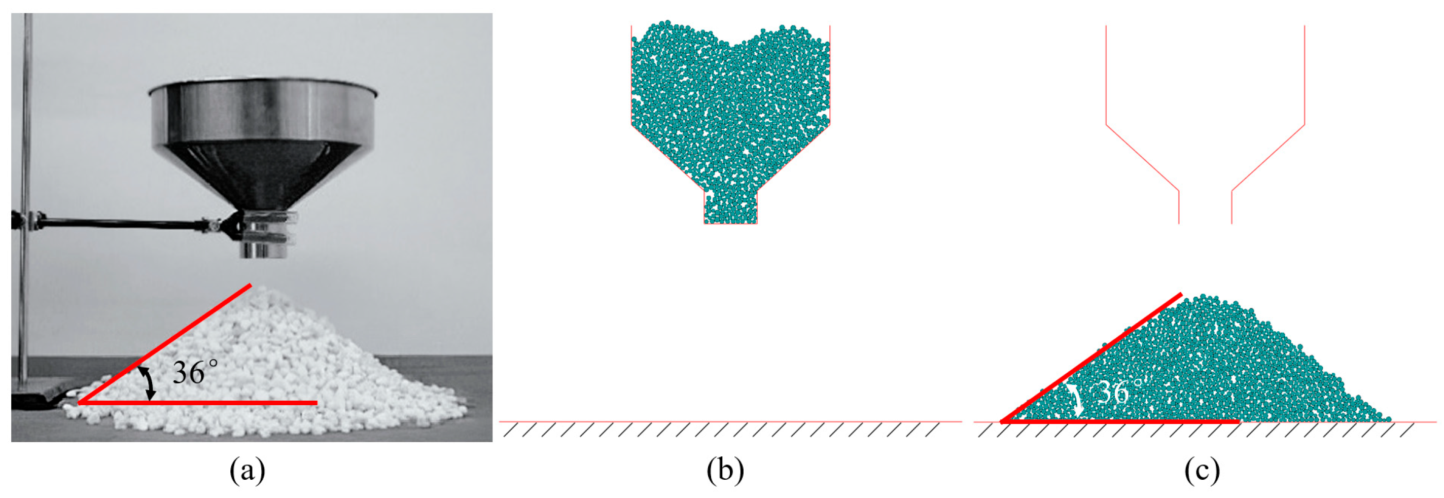
The natural angle of repose was determined via the collapse method using Particle Flow Code (PFC 2D) software (version 6.0; Itasca Consulting Group, Inc., Minneapolis, MN, USA). A schematic of the numerical setup is illustrated in Figure 1. A certain quantity of particles is generated above a fixed-funnel, gradually filling it under the action of gravity. The funnel gate is then opened, allowing the particles to flow out and accumulate beneath the funnel, forming a pile. The angle of repose of the pile is measured and compared with that obtained from physical experiments. Based on the deviation between the simulated and experimental angles, the microscopic parameters are iteratively adjusted. This trial-and-error procedure is repeated, with parameters being systematically refined in each iteration, until the simulated angle of repose converges to the experimental value within an acceptable tolerance, indicating that the macroscopic mechanical behavior of the particles is realistically captured. The parameters of ore particles, interburden particles, and waste rock particles are all calibrated using this method. After extensive trials and iterative adjustments, the final calibrated parameters are listed in

Table 1. Parameter setting of isolated ore-drawing experiment.

Particle	kn (N/m)	ks (N/m)	Density (kg/m3)	Fric	Damp	rr_fric
ore	5 × 107	5 × 107	3700	0.45	0.30	0.45
waste	1 × 108	1 × 108	2700	0.50	0.50	0.50
interburden	1 × 107	1 × 107	3000	0.40	0.45	0.43

. This procedure ensures that the DEM model reliably reproduces the bulk mechanical behavior and flow characteristics of the materials under study.

Parameters are adjusted, and the procedure is repeated until the simulation results match the experimental observations. The parameters of ore particles, interburden particles, and waste rock particles are all calibrated using this method. After extensive trials, the final calibrated parameters are listed in Table 1. The micro-mechanical parameters are defined as follows: kn and ks represent the normal stiffness and shear (tangential) stiffness of particle contacts, respectively, with units of N/m. Density (kg/m³) represents the mass density of individual particles. fric represents the contact friction coefficient between particles (dimensionless), controlling the resistance to sliding at particle contacts. Damp represents the local damping coefficient (dimensionless), which governs energy dissipation during particle collisions. rr_fric represents the rolling resistance coefficient (dimensionless), representing the resistance to particle rotation at contacts.

2.2. Construction of the Ore-Drawing Dataset with Interburden

A single-hole ore-drawing numerical simulation was conducted using a 1:100 scale model. The model dimensions were 800 mm × 1000 mm (length × height), with a 40 mm wide ore-drawing opening located at the center of the base. Approximately 8000 particles were included in the simulation. To prevent excessive particles overlap that could induce unrealistically high velocities, particles were initially distributed uniformly at random. A gravitational acceleration of 9.8 m/s² was applied, allowing the particles to settle under gravity and reach an initial equilibrium corresponding to natural piling.

2.2.1. Post-Defined and Pre-Defined Interburden Models

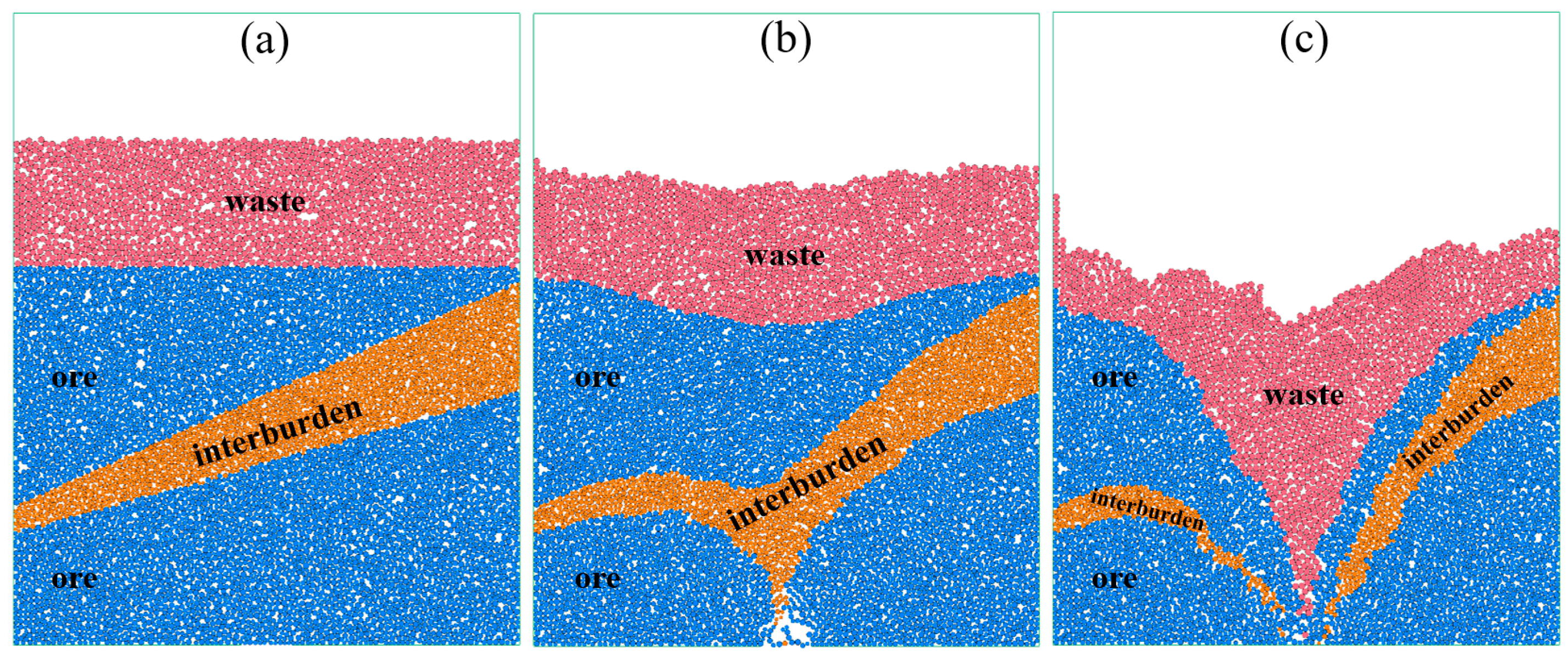
As shown in Figure 2, the generation of the pre-defined interburden model involves the following steps: (a) First, ore particles are generated up to a height of 0.8 m. (b) After reaching equilibrium, particles above the lower boundary are removed, and a wall is created at the lower boundary position. (c) Particles with specific properties are generated in the height range of 0.6–1.0 m. After equilibration, particles above the upper boundary are removed, and a wall is created at the upper boundary. (d) Waste rock particles are generated in the height range of 0.6–1.0 m. After equilibration, particle above 0.8 m are removed, and the walls at both the upper and lower boundaries are removed. After a subsequent equilibration, the initial pre-defined model is obtained. The ore-drawing simulation process using the pre-defined model is shown in Figure 3.

The numerical model was established under a two-dimensional plane strain assumption. Rigid walls were applied at the left, right, and bottom boundaries to restrict lateral and basal particle movement, while the top boundary was left free to allow gravity-driven deposition and flow. Gravity was the only external load applied in the simulations, with a gravitational acceleration of 9.8 m/s². Different geological layers were represented by assigning distinct particle properties (e.g., density, contact stiffness, and friction coefficient) rather than by defining explicit geometric interfaces. Interactions between different layers were governed by particle–particle contacts, and the mechanical behavior at layer boundaries emerged naturally from contacts between particles with different properties. Prior to ore drawing, particles were allowed to settle under gravity until a quasi-static equilibrium state was reached, after which the ore-drawing process was initiated.

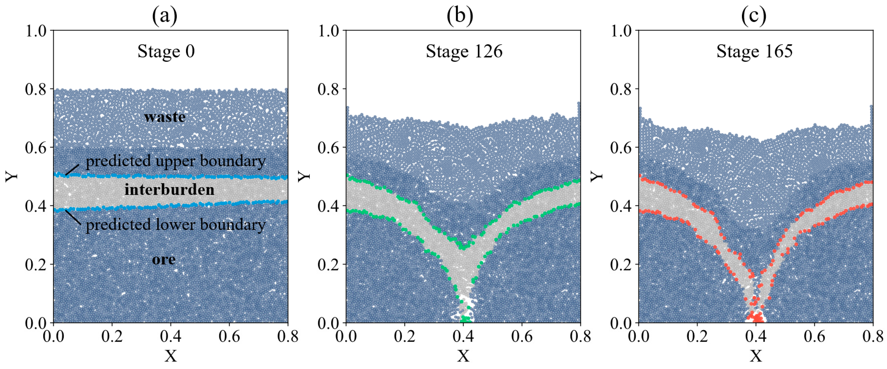
The ore-drawing process is halted when the waste rock particles, representing the covering layer (above 0.6 m), are first released. The simulation process for ore drawing using the pre-defined model is illustrated in Figure 3. Since the position and morphology of the interburden are neither fixed nor uniform, its shape evolution before and after ore drawing still follows a traceable pattern. The interburden, defined as a collection of specific particles, generally spans the ore-drawing zone of a single-hole model. This collection can be represented as the region bounded by upper and lower boundaries. Therefore, by determining the morphological changes in these two boundary lines before and after ore drawing, the evolution of the interburden can be obtained.

For the numerical simulations of the pre-defined interburden, it is sufficient to record the states of particles along the upper and lower boundaries of the interburden at all stages to obtain the corresponding dataset. However, since the position and morphology of the interburden are neither fixed nor uniform, each generation of the specific particle collection model requires predefining the upper and lower boundaries, followed by stepwise particle generation. Moreover, such simulations can only represent a single multilayer interface scenario. To obtain a large dataset under diverse conditions, extensive simulations would be required, resulting in significant computational cost.

Considering the complexity and computational time of model generation and calculation, using pre-defined interburden models is not conducive to acquiring sufficient data for training deep learning models. Therefore, we adopt an alternative approach: a particle collection model without interburden is first generated, and the states of all particles are recorded at all stages. Subsequently, by randomly setting the upper and lower boundaries, large amounts of post-defined interburden data with varying interface morphologies can be obtained. Following the concept of transfer learning [23,24,25], the easily accessible and large-scale post-defined interburden dataset is first used for pretraining to acquire reasonably optimized weights. These weights are then transferred through fine-tuning using the smaller, but more production-representative pre-defined interburden dataset to achieve higher accuracy.

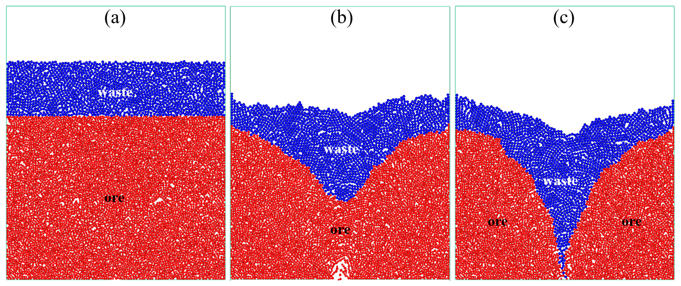
The generation of the post-defined model involves the following steps: first, ore particles are generated up to a height of 0.8 m. After equilibration, particles above 0.6 m are removed. Next, covering layer waste rock particles are generated in the height range of 0.6–1.0 m. After another equilibration, particles above 1.0 m are removed. The stopping condition for ore drawing is the same as that of the pre-defined modesl. The ore-drawing simulation process of the post-defined model is illustrated in Figure 4.

2.2.2. Building Datasets

In both the pre-defined and post-defined models, a Cartesian X–Y coordinate system is established on the two-dimensional plane, with the boundary lines represented as two continuous lines within this coordinate system. For the pre-defined model, the upper and lower boundaries correspond to the topmost and bottommost particles of the interburden particle collection. For the post-defined model, two boundary lines are randomly generated within the range x, y ∈ (0, 0.8 m), with the upper boundary always positioned above the lower boundary, thereby representing the region of the specific particle collection. The morphology of randomly generated upper and lower boundaries is illustrated in Figure 5.

The particle coordinate changes are recorded as ${(X_i^n,Y}_i^n)$, where $(X,Y)$ denotes the particle coordinates, $n$ represents the stage during the ore-drawing process, and $i$ is the particle ID. Starting from the beginning of ore drawing, the coordinates of particles are recorded every time 10 particles are released, and each such recording is designated as one stage. In all ore-drawing simulation experiments, the total number of stages $n_{max}$ exceeds 200.

Additionally, 81 points are selected along the X-axis at 10 mm intervals starting from 0, ensuring that each X value maps to a unique Y value. Thus, each boundary line is characterized by the coordinate variations of 81 uniformly spaced particles, representing the morphological changes in the interburden before and after ore drawing. The selection method of the candidate particle set $F_t$ is given as follows:

$$F_t=\left\{p_i\in P_{layer}|\left|x_i-x_t\right|\le \epsilon \right\}$$

(1)

Here, $p_i$ = ${(X_i^{n=0},Y}_i^{n=0})$ denotes the coordinates of the $i$-th particle at the initial stage. $P_{layer}$ represents the collection of all interburden particles, and $x_t$ is the $t$-th sampling position along the X-axis. For each sampling point, particles belonging to the interburden group are searched within a tolerance of $\epsilon$ = 0.015.

If no particle is found within this range, the particle $p_{i^{\mathrm{*}}}$ with the minimum horizontal distance to the sampling point is selected and added to the candidate set $F_t$.

$$F_t=\left\{p_{i^{*}}\right\},i^{*}=arg{min}_j\left|x_j-x_t\right|$$

(2)

For each sampling point, the particles in $F_t$ that have not yet been selected are evaluated to identify the particle with the maximum vertical coordinate $Y\left(p\right)$ as the upper boundary particle, and the particle with the minimum vertical coordinate $Y\left(p\right)$ as the lower boundary particle. The corresponding formulas are provided below. Once the boundary particles are determined, the dynamic changes in particle coordinates at each stage are recorded as dynamic inputs. Additionally, two static properties of the particles Radius ($R$) and Mass ($M$) are recorded as static inputs.

$$\left\{\begin{array}{c}{p}_t^{upper}=arg \underset{p\in F_t}{\mathit{max}}Y\left(p\right)\\ p_t^{lower}=arg \underset{p\in F_t}{\mathit{min}}Y\left(p\right)\end{array}\right.$$

(3)

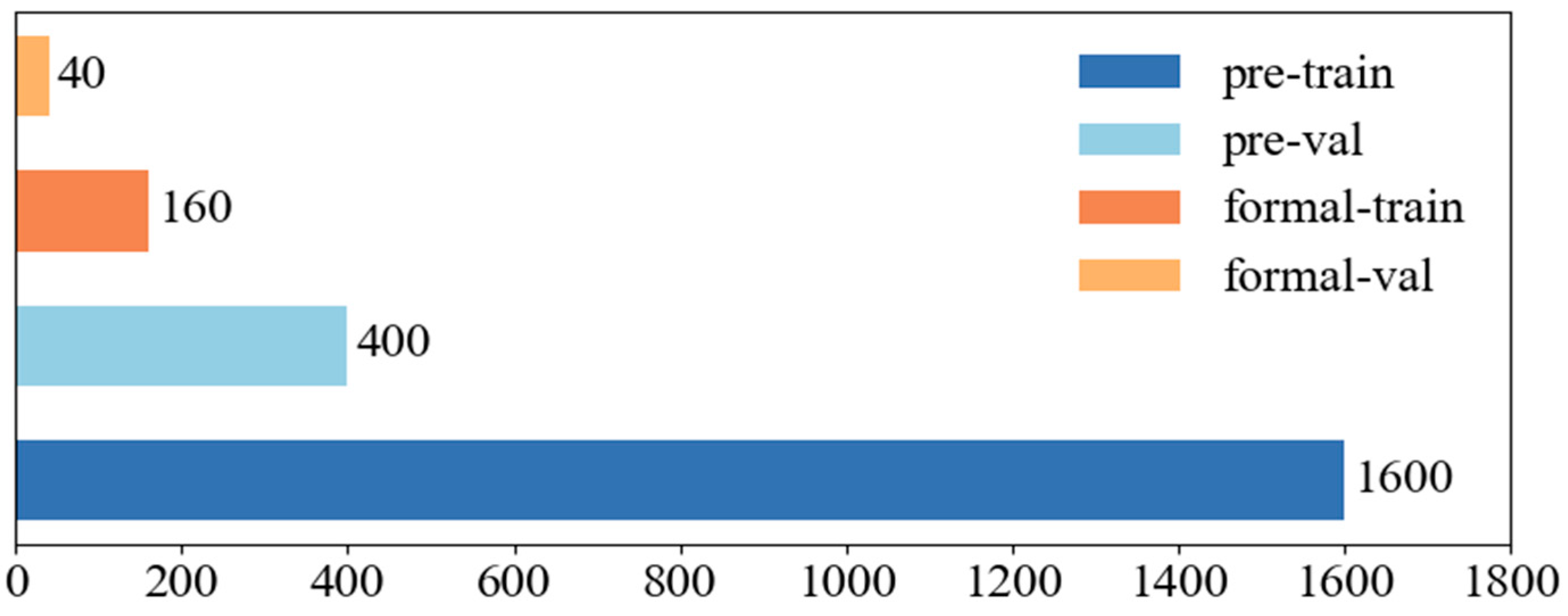
To achieve the initial objectives, the angle of repose determined from laboratory experiments was used to calibrate the parameters for numerical simulations, yielding the dataset required for this study. This dataset includes a large amount of post-defined interburden data and a smaller portion of pre-defined interburden data. Clearly, obtaining interface morphology data through autonomous delineation is relatively straightforward; however, post-defined interburden data cannot accurately reflect real conditions. A total of 2200 data samples were obtained, of which 2000 correspond to post-defined interburden and are used for pretraining, while 200 correspond to pre-defined interburden and are used for transfer learning. To ensure balanced evaluation of the subsequent network performance, 80% of the data in both pretraining and transfer learning were used for training, and 20% for validation. Detailed classification of data usage is presented in Figure 6.

3. Model

Granular flow during the ore-drawing process is inherently a spatiotemporally evolving phenomenon. In this typical spatiotemporal coupling problem of ore particle transport prediction, traditional physical models are constrained by simplified mechanical assumptions, while data-driven methods (such as LSTM), struggle to capture the nonlinear interactions among particle ensembles. The Transformer architecture [26], originally developed for natural language processing and time-series modeling, demonstrates unique advantages in sequence modeling tasks due to its self-attention mechanism and positional encoding system [27,28]. When applied to granular flow in ore drawing, the Transformer architecture enables joint modeling of the spatial positions of all particles at each stage, thereby uncovering the interaction and co-evolution patterns among particles. Its self-attention mechanism facilitates the capture of non-local dependencies, significantly enhancing the capability to model complex motion patterns.

3.1. Transformer Model

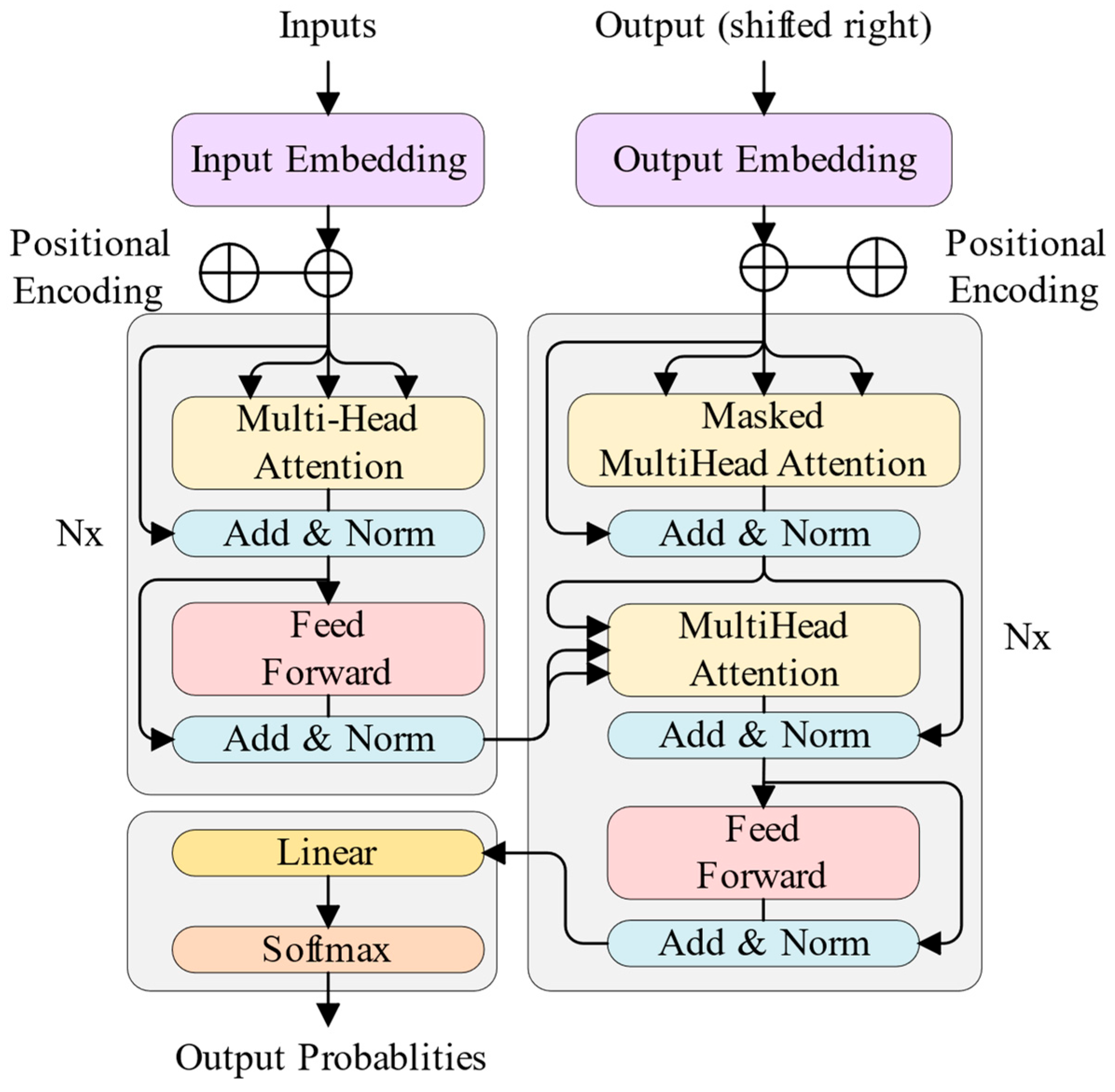
The fundamental architecture of the Transformer is illustrated in Figure 7. It consists of an encoder and a decoder, both constructed by stacking N identical layers [26]. The encoder is composed of two sublayers: (1) Multi-Head Self-Attention, which captures global dependencies among elements in the input sequence; and (2) the Position-wise Feed-Forward Network (FFN), which performs nonlinear transformations on features at each sequence position. Each sublayer adopts the standard structure of layer normalization → sublayer computation → residual connection, a design that substantially improves training stability and alleviates the vanishing gradient problem.

The decoder extends each layer into three sublayers: (1) Masked Multi-Head Self-Attention, where masking constrains each position to attend only to its preceding positions, thereby ensuring the causality of autoregressive generation; (2) Multi-Head Cross-Attention, where the queries are derived from the output of the preceding decoder sublayer and the keys/values are taken from the encoder output, thus enabling encoder–decoder information interaction; and (3) the Position-wise Feed-Forward Network (FFN).

In addition, the input and output modules include the Embedding Layer (which maps discrete symbols into dense vectors), Positional Encoding (which injects sequence order information through sinusoidal functions), and the final Linear and Softmax layers (which transform the decoder outputs into probability distributions over the target vocabulary). These components convert raw input text into representations processable by the model and generate the final outputs.

By eliminating recurrent and convolutional operations, this architecture relies purely on attention mechanisms to model long-range dependencies, thereby overcoming the sequential constraints of Recurrent Neural Networks (RNNs) and the locality limitations of Convolutional Neural Networks (CNNs).

However, the original Transformer architecture exhibits significant limitations in predicting granular flow during ore drawing in caving methods. Its insufficient spatiotemporal modeling capacity prevents a unified representation of two fundamentally distinct physical processes: instantaneous particle–particle interactions, which follow the principle of spatial simultaneity, and the evolution of individual trajectories, which is strictly governed by temporal causality. The attention mechanism, lacking explicit physical constraints, may inadvertently introduce information leakage from future states, thereby violating the core law of temporal irreversibility in granular motion. At the feature fusion level, the model adopts a single, simplistic integration strategy, making it ineffective in jointly incorporating static particle attributes with dynamically evolving positional information. Consequently, the influence of material properties on particle behavior cannot be accurately captured. Moreover, the architecture lacks a state-transition mechanism, rendering it incapable of simulating the critical shift from motion to rest when particles reach the drawpoint. This deficiency restricts the model’s ability to reflect physical priors and the staged release characteristics inherent in granular discharge. These limitations collectively constrain the predictive accuracy and physical plausibility of the original architecture in modeling the transport of interburden boundary particles during ore drawing.

3.2. Improved Transformer Model

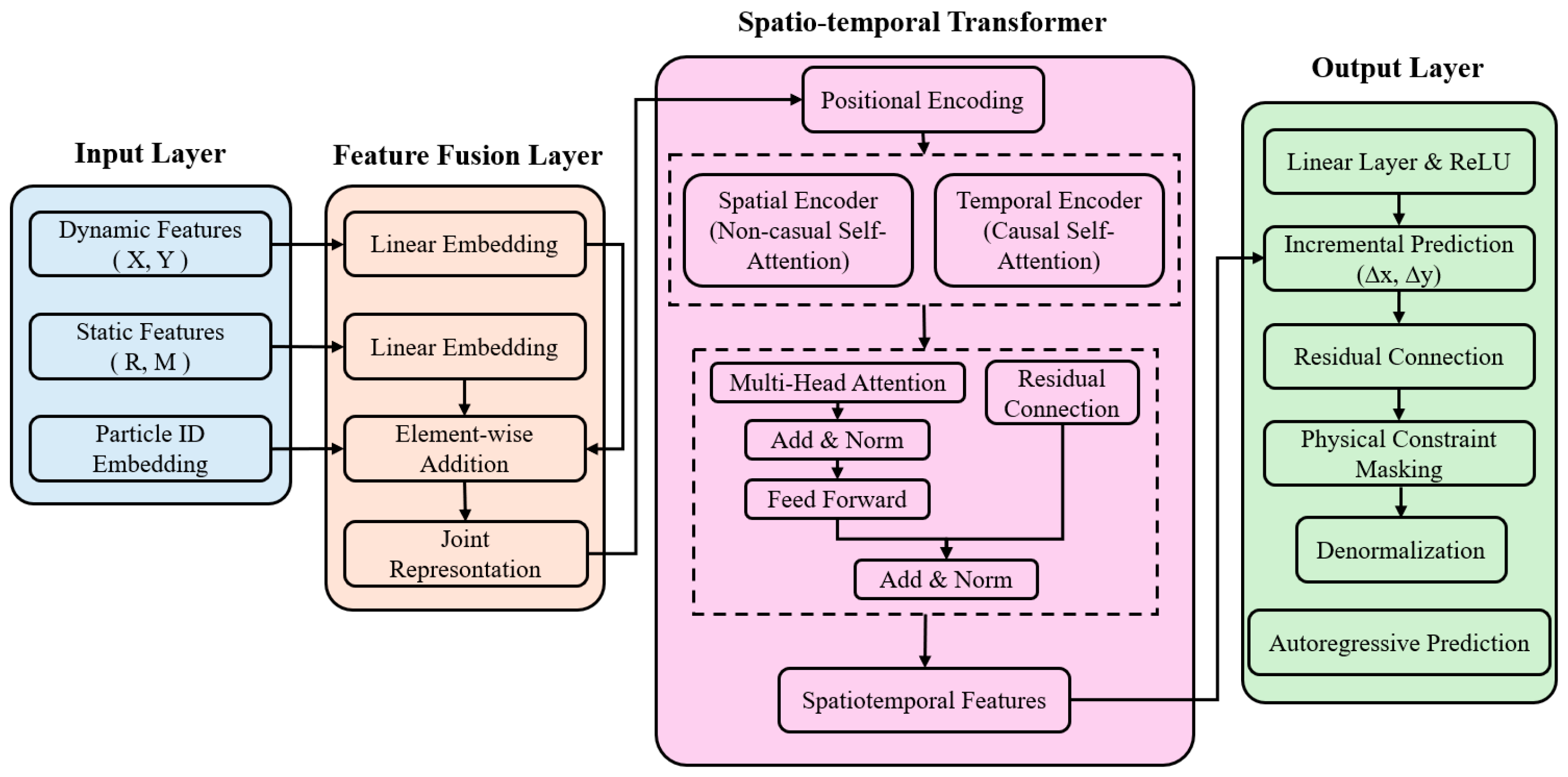
To overcome the limitations of the original Transformer in predicting ore–rock particle transport—namely, insufficient spatiotemporal modeling capacity, the lack of physical constraints in the attention mechanism, inadequate fusion of static and dynamic features, and the absence of a state-transition mechanism—this study proposes an improved Transformer model that integrates physical prior constraints. The overall model architecture is illustrated in Figure 8.

3.2.1. Input Stage and Feature Fusion Embedding

At the input stage, the architecture retains only the particle spatial coordinates $\left(X,Y\right)$ as dynamic features, while the particle $R$ and $M$ are treated as static features. Both static and dynamic features are independently normalized throughout the workflow to enhance numerical stability and generalization. This design discards redundant kinematic quantities that can be derived from positional differences, thereby reducing input dimensionality while emphasizing the physical attributes directly related to particle motion. In doing so, it avoids the accumulation of noise that could otherwise impair the accuracy of spatiotemporal modeling.

During the feature fusion embedding stage, the static features ${\mathrm{s}}_i$ and dynamic features ${\mathrm{d}}_i^{\left(t\right)}$ are linearly projected into a shared high-dimensional embedding space ${\mathbb{R}}^{{\mathrm{d}}_{\mathrm{model}}}$. The transformation is defined as

$$\left\{\begin{array}{c}{\mathrm{s}}_i^{\prime }={\mathrm{W}}_s{\mathrm{s}}_i+{\mathrm{b}}_s\\ {\mathrm{d}}_i^{\prime \left(t\right)}={\mathrm{W}}_d{\mathrm{d}}_i^{\left(t\right)}+{\mathrm{b}}_d\end{array}\right.$$

(4)

where $W_s,W_d\in {\mathbb{R}}^{{\mathrm{d}}_{\mathrm{model}}\times 2}$ denote the projection matrices for static and dynamic features, and ${\mathrm{b}}_s,{\mathrm{b}}_d\in {\mathbb{R}}^{{\mathrm{d}}_{\mathrm{model}}}$ are the corresponding bias vectors.

To integrate static attributes into temporal sequence modeling, the static embedding ${\mathrm{s}}_i^{\prime }$ is replicated along the time dimension and added element-wise to the dynamic embedding ${\mathrm{d}}_i^{\prime \left(t\right)}$. This operation yields the joint representation $f_i^{\left(t\right)}$, which reflects the modulation effect of inherent particle properties on instantaneous motion:

$$f_i^{\left(t\right)}=s_i^{\prime }+d_i^{\prime \left(t\right)}$$

(5)

In addition, particle ID embedding ${\mathrm{p}}_i$ is introduced, assigning each particle a unique learnable identifier. This mechanism captures individual physical heterogeneity and strengthens the model’s particle-level discrimination. The final feature input $z_i^{\left(t\right)}$ is expressed as follows:

$$z_i^{\left(t\right)}=f_i^{\left(t\right)}+p_i=W_s{s}_i+b_s+W_d{d}_i^{\left(t\right)}+b_d+p_i$$

(6)

3.2.2. Spatio-Temporal Transformer

Within the backbone, the model adopts a Spatio-temporal Transformer structure composed of a Spatial Encoder (non-causal self-attention) and a Temporal Encoder (causal self-attention). The Spatial Encoder models instantaneous interactions among particles within a single time step, consistent with the principle of spatial simultaneity in particle motion. In contrast, the Temporal Encoder performs sequential modeling of trajectory evolution under the constraint of a causal mask $M_{\mathrm{causal}}$, ensuring that trajectory prediction strictly adheres to temporal causality and preventing information leakage from future states. The self-attention computation of the Temporal Encoder is defined as follows:

$${\mathrm{Attn}}_{\mathrm{temporal}}\left(\mathrm{Q},\mathrm{K},\mathrm{V}\right) = \mathit{softmax}\left({\displaystyle \frac{\mathrm{Q}{\mathrm{K}}^{\mathrm{T}}}{\sqrt{{\mathrm{d}}_{\mathrm{k}}}}} + {\mathrm{M}}_{\mathrm{causal}}\right)\mathrm{V}$$

(7)

Here, $Q, K, V\in {\mathbb{R}}^{{T\times d}_k}$ denote the query, key, and value matrices, respectively; $d_k$ is the dimension of the key vectors; and $M_{\mathrm{causal}}$ is an upper-triangular mask matrix that strictly prohibits access to future time steps. Temporal position information is explicitly injected through sinusoidal Positional Encoding (PE), defined as follows:

$$\left\{\begin{array}{c}{PE}_{(t,2i) = \mathit{sin}\left({\displaystyle \frac{t}{{\mathrm{10,000}}^{2i/d_{\mathit{model}}}}}\right)}\\ {PE}_{(t,2i+1) = \mathit{cos}\left({\displaystyle \frac{t}{{\mathrm{10,000}}^{2i/d_{\mathit{model}}}}}\right)}\end{array}\right.$$

(8)

where $t$ denotes the time step, $i$ indexes the embedding dimension, and $d_{\mathrm{model}}$ is the dimensionality of the model embedding space.

3.2.3. Output Stage

At the output stage, the model adopts an incremental prediction strategy, predicting displacement increments $\left(∆x,∆y\right)$ instead of absolute coordinates. Trajectories are iteratively generated using residual connections, ensuring that the prediction form remains consistent with the physical motion process. The formula is shown as follows:

$${\widehat{\mathrm{d}}}_i^{(t+1)}=d_i^{\left(t\right)}+{∆\widehat{\mathrm{d}}}_i^{(t+1)}=d_i^{\left(t\right)}+\mathrm{M}\mathrm{L}\mathrm{P}\left(h_i^{\left(t\right)}\right)$$

(9)

Furthermore, to account for the physical process of state transitions during particle release in ore-drawing simulations, a Physical-Constraint-Masking (PCM) mechanism is introduced. In autoregressive prediction, once a particle is determined to be released at a given stage, its subsequent predicted positions are fixed at the release coordinates, and these positions are masked during loss computation. This ensures that particle state predictions adhere closely to the true evolutionary process.

Through these design choices, the improved spatiotemporal Transformer not only retains the original Transformer’s advantage in modeling global dependencies, but also incorporates innovative, physics-driven components—feature selection guided by physical priors, particle ID embedding, spatial–temporal dual encoding, incremental prediction, and release-state physical constraints. Collectively, these enhancements enable high-precision prediction of interburden boundary particle transport during ore drawing and physically consistent modeling of ore–rock granular flows, providing both theoretical support and a practical implementation pathway for intelligent prediction of complex granular systems.

4. Experiment

4.1. Model Training

The data acquisition has been completed, yielding a large dataset under post-defined interburden conditions and a smaller dataset under pre-defined interburden conditions. Evidently, obtaining interface morphology data through autonomous delineation in the post-defined interburden scenario is relatively straightforward. However, these data differ somewhat from those under pre-defined interburden conditions and cannot accurately reflect the actual situation. Therefore, a transfer learning strategy was adopted. The post-defined interburden dataset was used for pre-training, and transfer learning was subsequently applied to further train the pre-defined interburden dataset. Specifically, the former serves to pre-train the model to rapidly obtain reasonably optimal weights for this task, while the latter fine-tunes these weights to achieve more precise task-specific performance.

The training data consist of particle trajectory time series, with each sample containing 162 particles and recording their two-dimensional spatial positions over 200 steps. Input features were strictly selected based on physical relevance: static features include particle $R$ and $M$, while dynamic features consist solely of the two-dimensional coordinates $\left(X,Y\right)$ at each time step. Redundant kinematic variables such as velocity and acceleration, which can be derived from positional differences, were excluded to ensure the model focuses on the intrinsic patterns of particle spatial migration.

The improved Transformer model has a feature dimension of 128, attention heads of 8, and a feedforward network dimension of 512. Model parameters are optimized using the Adam optimizer. The initial learning rate is set to 10⁻⁴, and after 50 epochs of warm-up training, cosine annealing is applied for fine-tuning, with a minimum learning rate of 10⁻⁶. An early stopping mechanism is employed to prevent overfitting, terminating training if no improvement occurs within 30 epochs. Data without interburden are used for pre-training, whereas data with interburden are used for transfer learning. The parameter settings for pre-training and transfer learning are largely consistent, with minor differences. Detailed configurations of model and training parameters are presented in

Table 2. Hyperparameter settings of the deep learning model: all parameters are dimensionless neural network architecture hyperparameters commonly used in artificial neural network and Transformer-based studies.

Model		Train
Parameter	Value	Parameter	Value
input_features	5	num_points	162
output_features	8	dropout	0.1
d_model	256	epochs	250
n_head	8	batch_size	16 (4, transfer learning)
num_layers	6	learning_rate	10−4 (10−5, transfer learning)
dim_feedforward	1024	weight_decay	10−5

.

During training, a physics-constrained masking mechanism was introduced, such that loss is computed only for particles that have not yet been released and their corresponding stages. A mask matrix $M_{\mathrm{valid}}\in {\left\{\mathrm{0,1}\right\}}^{N\times T}$ is defined, where ${\mathrm{M}}_{\mathrm{valid}}\left(i,t\right)=0$ if particle $i$ is in a released state at time $t$, and $M_{\mathrm{valid}}\left(i,t\right)=0$ otherwise. Accordingly, the loss function is formulated as the Masked Mean Squared Error (MMSE):

$$MMSE={\displaystyle \frac{{\sum }_{i=1}^N{\sum }_{t=1}^T{M}_{valid}(i,t)·{‖{∆d}_i^{\left(t\right)}-∆{\widehat{d}}_i^{\left(t\right)}‖}_2^2}{{\sum }_{i=1}^N{\sum }_{t=1}^T{M}_{valid}(i,t)}}$$

(10)

where ${∆d}_i^{\left(t\right)}$ and $∆{\widehat{d}}_i^{\left(t\right)}$ represent the true and predicted displacement increment vectors, respectively. The masking strategy particularly retains the prediction error at the instant of particle release to improve model accuracy at critical release points.

The experiment was conducted on a computer platform running Windows 10, equipped with an Intel (R) Core (TM) i7-11700 processor (Intel Corp., Santa Clara, CA, USA), an NVIDIA GeForce RTX 3090 graphics card (Santa Clara, CA, USA), and 32 GB of RAM. The network model was built using the Python 3.9 interpreter, leveraging GPU acceleration to enhance segmentation accuracy and speed. The variations in training and validation Loss and Grad during the pre-training and transfer training processes are shown in Figure 9. Both the loss values and gradients exhibit a continuous decrease and eventual convergence. Compared with pre-training, transfer training demonstrates a faster loss reduction while converging to a similar level, indicating that transfer training enables more efficient knowledge transfer across similar samples and facilitates a more precise reconstruction of model weights, thereby enhancing both convergence efficiency and predictive accuracy.

4.2. Results and Analysis

4.2.1. Model Prediction Performance Evaluation

To evaluate the effectiveness of the improved Transformer model in predicting multi-layer interburden particle migration, an independent validation set was employed. To avoid evaluation bias caused by inconsistent data distributions, both static and dynamic features were standardized using the training set statistics (mean and standard deviation), and the same normalization parameters were applied during validation and inference.

Unlike the single-step prediction mode used during training, the evaluation adopts a sequential prediction mode. Specifically, the particle states at stage $t$ are used to predict stage $t+1$, which then serves as the input for the next prediction, iteratively. This approach mitigates the interference of long-term accumulated errors on parameter updates and reflects the model’s stability in long-horizon sequence prediction under realistic inference conditions.

The evaluation metric is the normalized Euclidean error $E$, which is defined as

$$E={\displaystyle \frac{1}{D}}·{\displaystyle \frac{1}{N}}\sum _{i=1}^N{‖d_i^{(n+1)}-{\widehat{d}}_i^{(n+1)}‖}_2$$

(11)

where $d_i^{(n+1)}$ and ${\widehat{d}}_i^{(n+1)}$ denote the true and predicted two-dimensional positions of particle $i,$ respectively.

Figure 10 presents the prediction error curves of four validation samples under different interburden conditions during the ore-drawing process. In Stage 0–50, all samples exhibit low-amplitude, steadily increasing errors, with initial errors close to zero, indicating that the model accurately reproduces the slow displacement characteristics of particles during this stage. At Stage 50, the error values of all four samples are highly similar, demonstrating the model’s strong capability in capturing the trajectories of constrained particles. During Stage 50–100, as some particles gradually approach and exit the ore drawpoint, the error curves display slight fluctuations but continue to rise steadily, with the growth rate of the error relatively reduced. In Stage 100–150, additional boundary particles reach the ore drawpoint and are released, causing further increases in error; the four sample curves show more noticeable fluctuations and greater variability, likely due to differences in interburden morphology among the samples. Nevertheless, the overall error growth rate continues to slow. In Stage 150–200, the overall error level rises further but at a decelerated rate. Benefiting from the physics-constrained masking mechanism in the loss function, the model maintains high prediction accuracy even after a large number of particles are released, without abrupt error spikes. At Stage 200, the error values across different samples remain similar, indicating good generalization of the model in learning particle migration across varying samples. These results demonstrate that the improved Transformer model not only effectively captures the overall migration trends under multi-layer interburden conditions but also preserves prediction stability for particles with highly dynamic coordinates.

4.2.2. Particle Coordinates Prediction and Analysis

Figure 11 presents the true and predicted coordinates of interburden boundary particles at stages 0, 50, 100, and 200 during the ore-drawing process for four samples. As shown, the spatial distribution predicted by the model closely matches the true distribution. In particular, at Stage 50 and Stage 100, the model accurately captures the particle positions at these stages. At Stage 200, although particle motion becomes more complex due to boundary perturbations and inter-particle collisions, minor deviations occur near some release points. Nevertheless, the overall trend of particle curves remains highly consistent, demonstrating excellent predictive performance.

However, near the ore drawpoint, the predicted vertical coordinates of particles tend to cluster around the average values of the previous stage before release, rather than exhibiting the smoother divergence seen in the true coordinates. This discrepancy arises from the model’s attempt to balance the abrupt state transitions of particles before and after release, and it corresponds statistically to the mean positions of particles in the pre-release stage.

Across the initial, mid, and near-terminal stages of ore drawing, the model consistently reproduces the collective motion patterns of particles, indicating strong spatiotemporal modeling capability and effective representation of complex particle interactions.

4.2.3. Particle Trajectory Reconstruction and Analysis

By extracting the coordinates of interburden boundary particles at each stage, the migration trajectories of particles from the initial stage can be reconstructed. Figure 12 presents the true and predicted trajectories of interburden boundary particles at stages 0, 50, 100, and 200 during the ore-drawing process for four samples. In the spatiotemporal prediction task of ore particle flow trajectories, although the true particle motions exhibit nonlinear, non-stationary characteristics with significant disturbances due to complex multi-body interactions, collisions, and frictional effects, deep learning–based predictive models generally output smoother, approximately linear trajectories. This phenomenon is evident in the experimental results, where the predicted particle paths lack the high-frequency fluctuations and random offsets observed in the true trajectories, instead reflecting an idealized principal trend.

The fundamental cause of this phenomenon can be attributed to the adoption of Masked Mean Squared Error (MMSE) as the loss function during model training. When modeling highly uncertain and diverse physical processes, this loss formulation drives the model toward predicting the mean trajectory over all possible realizations of the true paths. Since the actual trajectories of ore particles may vary under identical initial conditions—due to different stochastic perturbations—the MMSE objective treats such variations as noise and effectively smooths them out. Consequently, the model learns an “averaged” trajectory rather than capturing any specific realization. Moreover, deep neural network architectures intrinsically tend to suppress high-frequency fluctuations and emphasize dominant trends when stochasticity or multi-modal distributions are not explicitly incorporated. This inherent bias further amplifies the smoothing effect in trajectory predictions. Additionally, the dataset commonly contains only a single observed trajectory per initial condition, lacking adequate sampling of the diverse perturbation scenarios that may occur under the same initial state. Such a “single-label” training paradigm implicitly assumes a deterministic relationship, thereby constraining the model to learn a one-to-one mapping from inputs to outputs. This limitation prevents the model from representing the inherent stochasticity and variability of the underlying physical process.

Nevertheless, this trajectory smoothing has limited impact on the objectives of this study, as the primary focus is on the overall trends of particle motion and positional changes at critical stages. Although MMSE leads to smoother trajectories, it emphasizes fitting the main trend, thereby improving the accuracy and stability of particle position predictions at key stages. As a result, the model effectively supports analysis of the macroscopic patterns and critical events in ore particle flow.

4.2.4. Prediction and Analysis of Key Nodes of Drawn Ore Grade Change

For scenarios involving interburden, the grade of interburden differs from that of the ore (here assumed to be lower than the ore grade). As shown in Figure 13, the drawn ore grade undergoes changes during the ore-drawing process, typically passing through four key nodes (such as ①) —though in some samples with extreme interburden morphology and positions, only two or three nodes may occur (such as ② and ③). Starting from the initial node (a), the drawn ore grade reaches a mutation node (b), where the lower boundary curve of the interburden above the ore drawpoint fractures. The mixing of interburden causes an abrupt drop in grade followed by a sustained decline. There may also be a lowest node (c) and a recovery node (d). The lowest node (c) generally occurs when the upper boundary curve of the interburden above the drawpoint fractures. As the ore particles above the upper boundary are released, the drawn ore grade reaches its lowest value and begins to rebound. After the recovery node (d), no interburden particles are released, and the drawn ore grade returns to the ore grade.

Among these stages, the mutation node (b) and the lowest node (c) are particularly important for guiding early-stage production operations on-site. Accurate prediction of these two key nodes can help operators better understand the state of the interburden and make more informed adjustments to production planning. Therefore, this study focuses primarily on analyzing the predictive performance at these two critical stages.

Figure 14 presents a case study of the prediction results for key nodes in drawn ore grade variation. In this case, the interburden upper and lower boundaries at the initial node (a) are represented by two straight lines, respectively. This figure illustrates the morphology evolution of ore, overlying waste rock, and interburden in the numerical simulation experiment. The mutation node (b) occurs at stage 126, and the lowest node (c) occurs at stage 165. The improved Transformer model predicts both key nodes at the same stages as those observed in the numerical simulation. The predicted positions of interburden boundary particles at these key nodes are marked as discrete points in the subplots. As shown in nodes (b) and (c), the predicted interburden boundaries closely match the interburden boundaries in the numerical simulation, demonstrating the model’s effectiveness in predicting particle positions at critical stages.

To further quantify the accuracy of interburden morphology prediction at the key nodes, the interburden upper and lower boundary particles were connected to delineate the interburden area. The predicted interburden areas at the key nodes for 40 validation samples were compared with the numerical simulation results. Benefiting from the positive effect of the physics-constrained masking mechanism on particle release state transitions, the predicted stages for these two key nodes are generally consistent with those in the numerical simulation, with a maximum stage discrepancy of only one stage. The area differences are presented in Figure 15. At the mutation node (b), most predicted area differences fall within ±0.01 m², whereas at the lowest node (c), the differences are slightly larger. Across samples, the area differences at the two nodes exhibit strong correlation. There is no consistent sign (positive or negative) for the differences across samples, which is related to the variability in interburden area at the initial stage in each sample. Overall, the mean percentage difference remains around 4%, indicating that the model achieves high reliability in predicting interburden area at critical nodes.

5. Conclusions

To address the complex problem of predicting boundary particle migration during ore drawing using the caving method with interburden, this study systematically investigates dataset construction and model design, experimentally validating the effectiveness of the proposed approach. The primary conclusions are as follows:

(1)

The dataset construction method proposed in this study employs numerical simulation experiments to achieve high-precision calibration of the angle of repose parameter. It establishes a single-hole ore-drawing numerical simulation dataset encompassing both “post-defined interburden models” and “pre-defined interburden models”. This approach effectively mitigates the challenge of insufficient data volume arising from difficulties in data acquisition under interburden conditions, and furthermore, delivers reliable support for model pre-training, transfer learning, and validation.

(2)

The improved Transformer model proposed in this study incorporates a multi-layer feature fusion embedding module at the input stage to enhance the spatiotemporal feature representation capability for particle migration. Within the backbone network, the spatiotemporal attention mechanism is reinforced to capture long-range dependencies. The decoder structure is optimized at the output end to improve the modeling capacity for local dynamic variations. The refined model achieves a more comprehensive characterization of the migration processes resulting from complex interactions among particles.

(3)

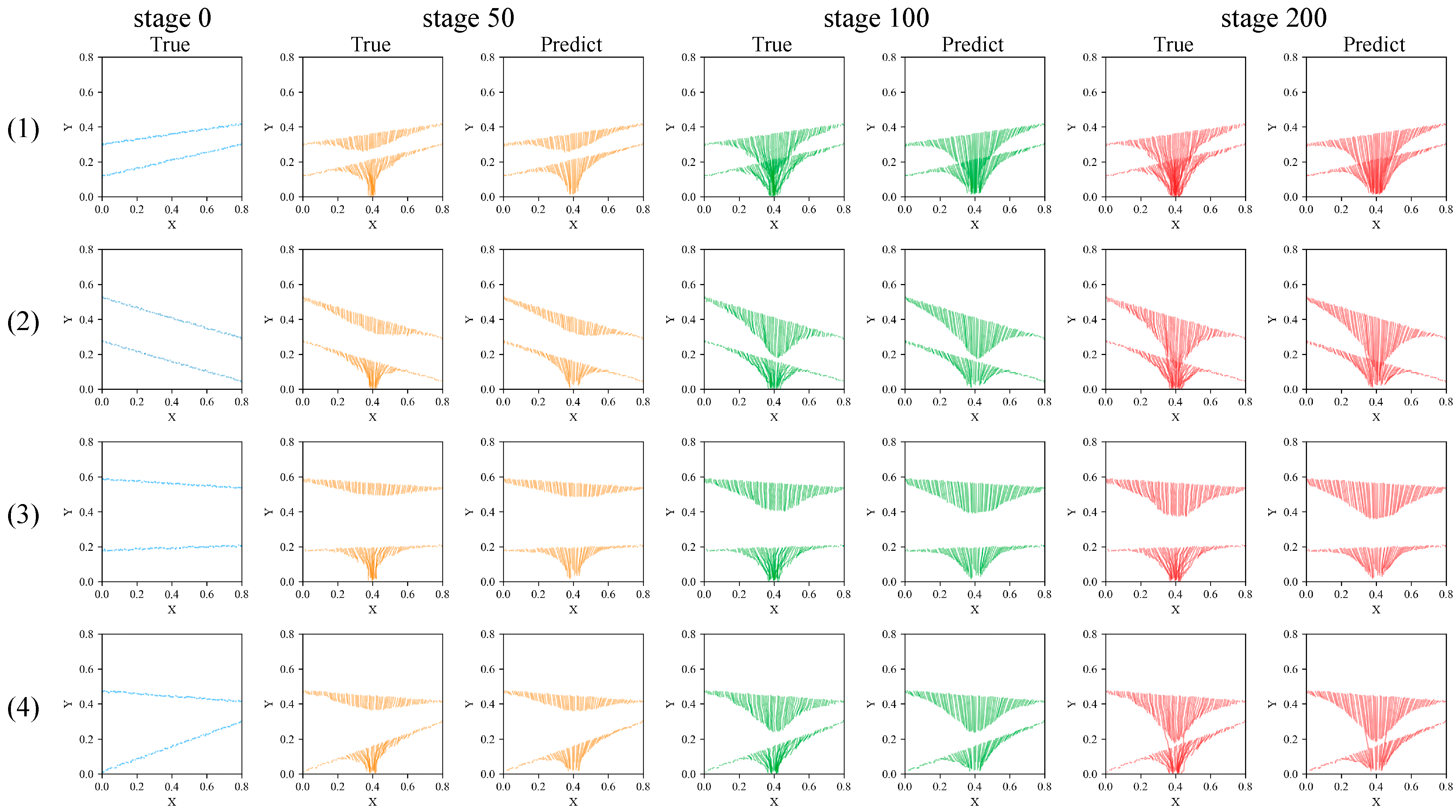
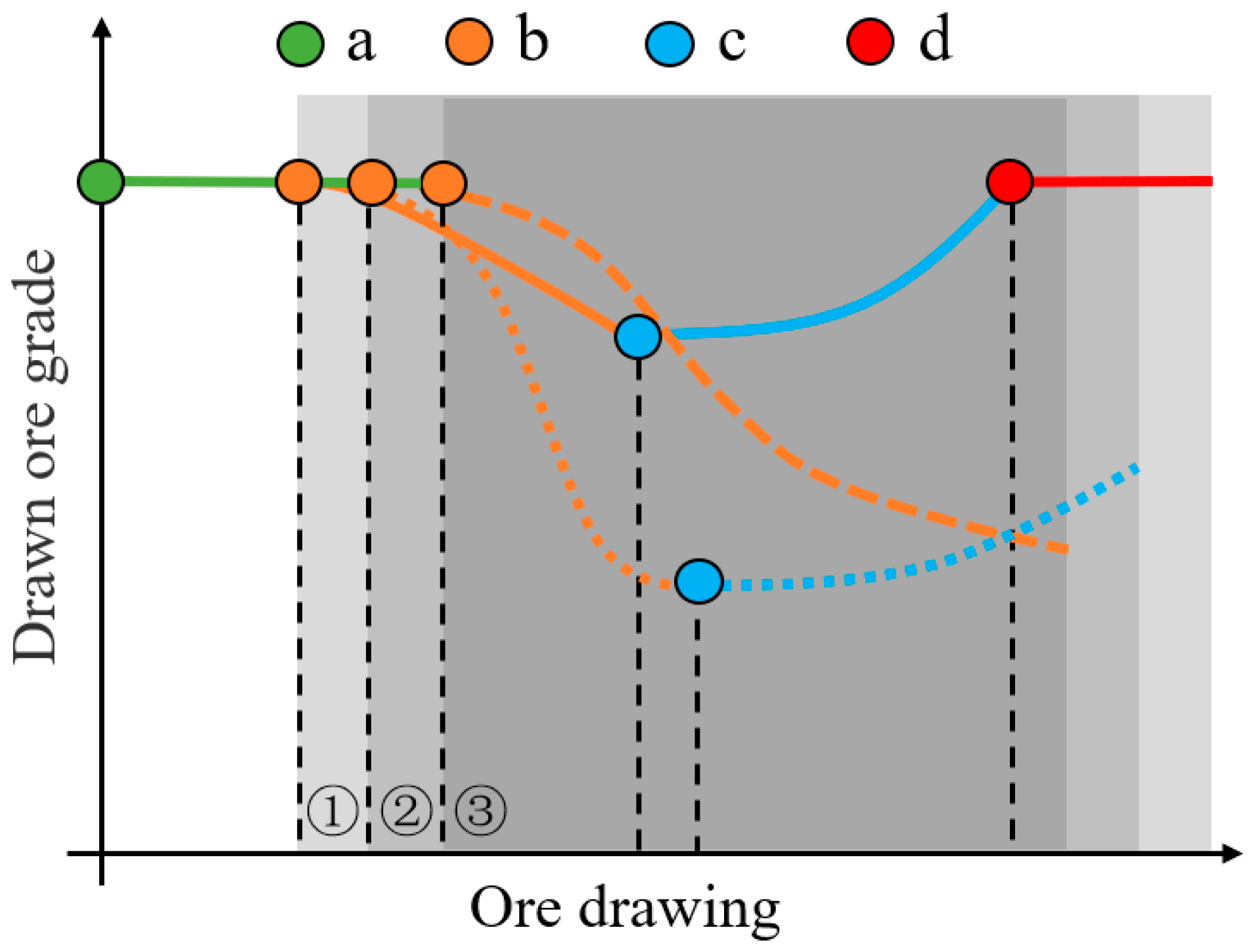
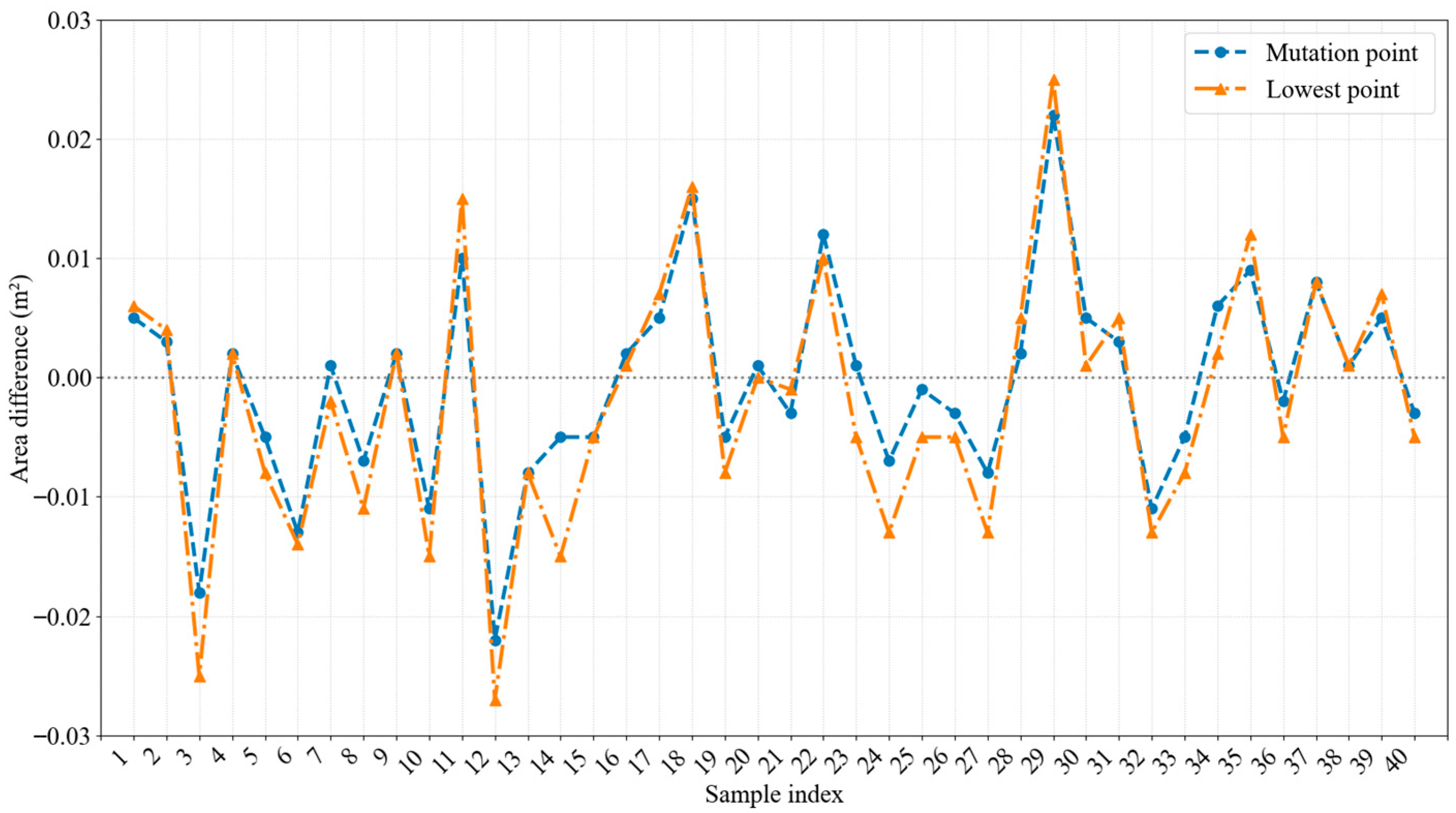
Operating in continuous prediction mode, the improved Transformer model demonstrates high prediction accuracy across various interburden samples within the dataset. It accurately reproduces the evolutionary trend of particle coordinates throughout the ore-drawing stages, indicating the model’s robust generalization performance. Concurrently, the model precisely identifies the critical stage numbers corresponding to changes in ore discharge grade. At these critical points, the average prediction error for interburden area is approximately 4%, confirming the model’s high reliability and practical value for forecasting key indicators.

Future research will prioritize the following directions: (1) extending the proposed framework to mines with different geological conditions, ore types, and ore-drawing configurations by expanding the model parameter space and incorporating mine-specific constraints, thereby enhancing the adaptability and generalizability of the approach to similar underground metal mines employing caving methods with interburden, and (2) continuously enriching the dataset by integrating field-measured data and high-fidelity numerical simulation results from different mining sites and further optimizing model performance through transfer learning and domain adaptation techniques, with the aim of achieving more robust, efficient, and broadly applicable predictions of boundary particle migration.