Quantitative Evaluation of Drilling Fluid Damage in Fractured Carbonate Reservoirs

Abstract

Ultra-deep fractured carbonate reservoirs suffer severe fluid loss and formation damage, requiring accurate characterization of natural fracture parameters and contamination behavior. Current field evaluation methods rely solely on logging data, which cannot obtain parameters such as the number and width of fractures. Taking the Shunbei Block as an example, this study integrates laser particle size analysis, HTHP flooding experiments, and a fracture loss model incorporating dynamic mud cake growth to clarify single-fracture loss behavior for fractures of different widths. Using fracture parameters interpreted from field logging, together with loss data and simulation results, we developed a method to determine fracture parameters and characterize contamination. Experiments reveal that effective plugging becomes difficult when fracture width exceeds 138 μm. Simulations indicate that cumulative loss volume increases with fracture width. The field loss volumes of 40–6600 m³ correspond to single-fracture widths of 0.9–6.2 mm. Based on the simulated width–loss volume relationship, correction coefficients for fracture count and width for two wells were calibrated. The method was applied to 9 wells, yielding an R² of 0.86 between predicted and measured loss volumes. The method effectively identifies fracture parameters and assesses contamination, supporting lost circulation control in fractured carbonate reservoirs.

1. Introduction

Carbonate reservoirs in the Tarim Basin, especially the ultra-deep fracture-cavity type in the Shunbei Oilfield (at depths of 7200–8800 m), have low matrix porosity (averaging 2.07%) and permeability (0.01–5.52 md) [1,2]. Consequently, the storage and flow capacity rely almost entirely on fractures, which connect to distant dissolution caves [3,4]. However, these fracture networks also make the reservoir highly susceptible to severe mud losses (39–6625 m³,

Table 1. Field lost volumes and skin factors.

Well	Drilling Fluid Lost Volumes (m3)	Skin Factors (Dimensionless)
A1	39	0.29
A2	756	15.5
A3	6625	15.1
A4	2138	9
A5	1985	16.3
A6	2666	12

), which often induce significant formation damage. Because the tight matrix offers little compensatory permeability, damage to these fracture systems directly translates to substantial productivity loss, making quantitative damage evaluation a critical necessity.

Accurately characterizing fracture width is thus critical. The main techniques for observing downhole natural fractures include core analysis, imaging logging, and conventional well logging. However, core analysis is costly [5] and often impractical in fractured reservoirs, where severe fluid loss and drilling breaks lead to poor core recovery or highly fragmented rock [6]. Imaging logs can directly characterize fractures, but suffer from subjective interpretation errors [7]. Although identification accuracy has been improved by advanced methods [8,9,10,11] and deep learning models [12,13], these techniques remain costly and do not provide continuous inter-well data. By contrast, conventional well logs are cost-effective and widely available across multiple wells, offering continuous data coverage. Consequently, field operations still rely primarily on conventional well logs for fracture prediction.

Conventional log-based predictions are inherently error-prone. Researchers have developed processing techniques to improve accuracy, e.g., integrating drilling fluid loss data for quantitative fracture width assessment [14], applying semi-supervised learning to achieve 98.3% accuracy in fracture detection [15], and combining wavelet denoising with fractal analysis to reduce heterogeneity errors [16].

However, log-only interpretation suffers from an inherent information deficit. The accuracy of such approaches is fundamentally constrained, highlighting the need to incorporate complementary data for reliable fracture characterization. Although some researchers have used loss data to validate log-based fracture predictions, few have integrated experiments, simulations, and field logs to correct predicted fracture parameters based on the physical processes of drilling fluid flow and plugging.

Numerical simulation is a primary tool for studying such mechanisms. Existing models include 1D linear, 1D radial, and 2D planar types [17]. 1D models cannot handle multiple fractures along a horizontal well. In contrast, the 2D planar model can handle multiple fractures concurrently, making it more suitable for studying drilling fluid damage. Ozdemirtas et al. [18,19] developed a 2D model specifically for H-B fluids, characterizing fracture roughness via fractal dimensions and fractional Brownian motion, and incorporating an exponential deformation law. Jia et al. [20] presented a 2D model for power-law fluids that couples linear fracture deformation, fracture roughness (via tortuosity and mechanical width), and wall filtration (Carter model) to predict fluid loss rate. In summary, existing models for drilling fluid loss primarily focus on fracture deformation, wall filtration, and fluid rheological properties.

With growing engineering attention to the magnitude of drilling fluid loss, several researchers have investigated the relationship between lost volume and fracture width. Li et al. [21] simulated this relationship under varying pressure differentials and validated it with laboratory experiments, but not with field data. In contrast, Dokhani et al. [22] used a 1D radial model for power-law fluids incorporating fracture deformation and wall filtration, and successfully predicted field loss volumes. Nevertheless, existing models primarily focus on drilling fluid invasion damage without incorporating experimental plugging mechanisms and have rarely been validated against field data. Although Ezeakacha and Salehi [23] investigated loss behavior with mud cake formation in porous carbonate rocks, their findings do not extend to natural fractures.

Field observations from the Shunbei Oilfield reveal that although natural fractures connect to caverns (implying continuous lost circulation), drilling fluid loss is self-limiting owing to fracture plugging. In fact, bridging and mud cake formation are effective mechanisms for mitigating severe lost circulation (>30 m³/h, [17]) in fractured reservoirs. However, a methodology that couples plugging mechanisms with experiments, simulations, and field data is still lacking for such severe loss conditions.

Therefore, this study proposes an integrated methodology that couples laboratory characterization of plugging mechanisms, numerical simulation of mud cake growth dynamics, and field-data-driven calibration of log-derived fracture parameters. It enables improved fracture prediction and supports plugging optimization.

2. Materials and Methods

2.1. Workflow

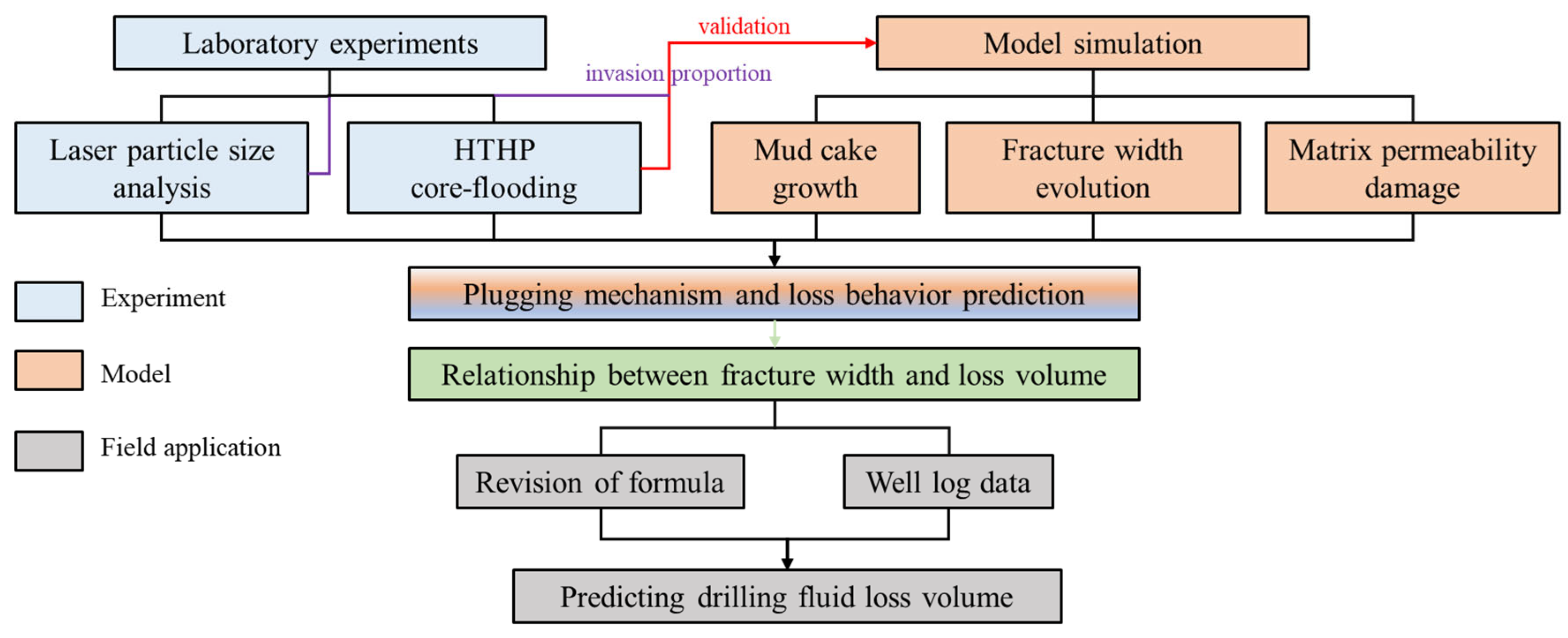
Quantifying drilling fluid loss parameters from conventional well logs is inherently difficult in the ultra-deep fractured carbonate reservoirs of the Shunbei Field. To address this, we combined laboratory experiments, fluid loss modeling, log interpretation, and field loss data analysis. Laser particle size analysis and HTHP core-flooding experiments characterized the solid-phase size distribution and loss behavior under varying fracture widths, revealing the plugging mechanism. A 2D planar fracture loss model incorporating dynamic mud cake growth, effective width evolution, and matrix permeability damage was developed and validated against experiments. From the model, we derived the relationship between fracture width and loss volume, which, together with conventional logs, was used to calibrate the existing width prediction formula against field loss data. This yielded recalculated fracture widths that successfully matched observed loss volumes, establishing a practical analysis framework for the studied block (Figure 1).

2.2. Experiments

To investigate the mechanism of drilling fluid loss and contamination, a laser particle size analyzer was employed to determine the PSD of the solid phase within the drilling fluid. Furthermore, fractured core damage experiments were conducted using an HTHP core flooding apparatus to analyze the damage behavior of the drilling fluid.

2.2.1. Samples Preparation

(1) Core samples

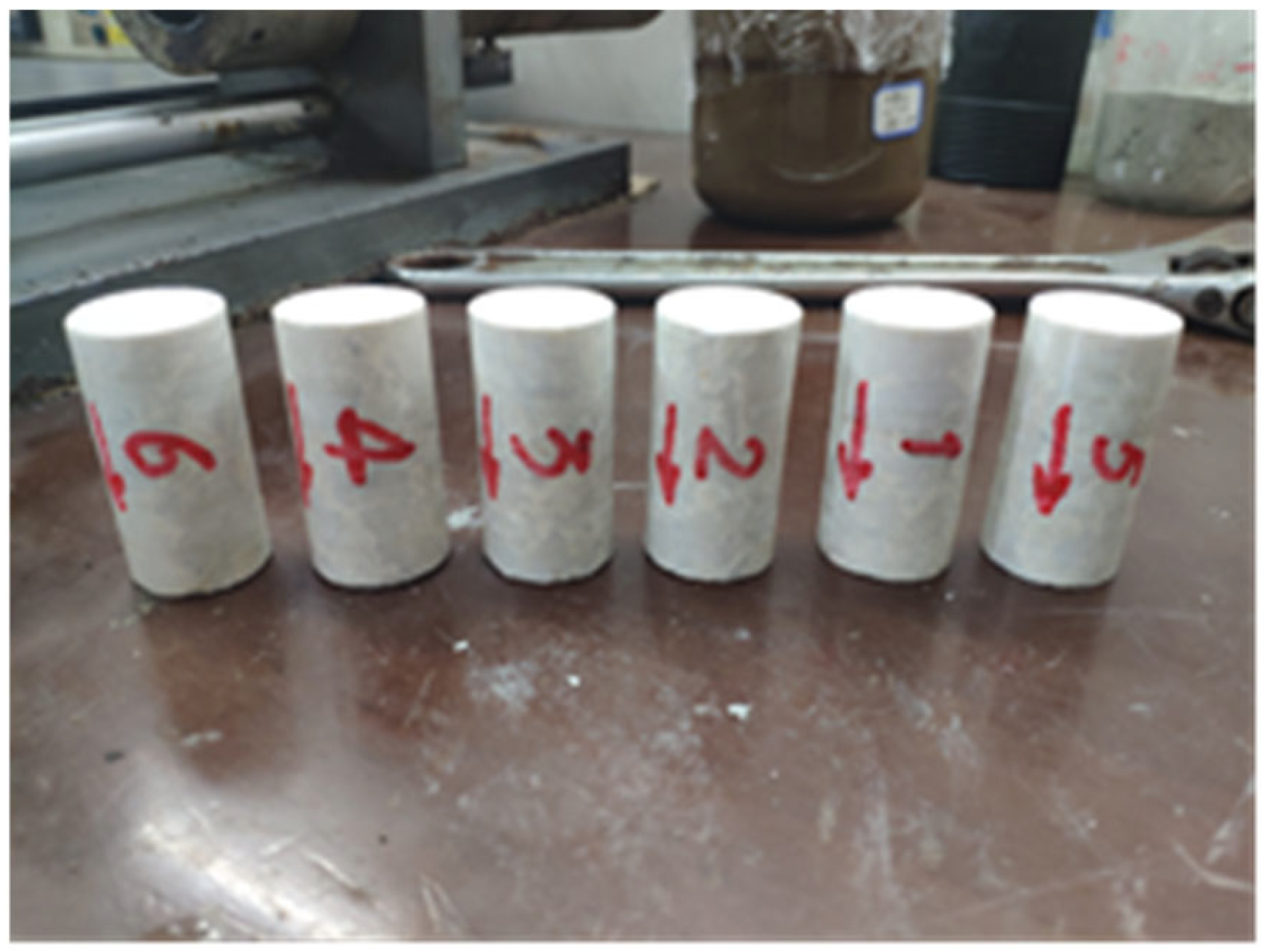
Twenty standard core plugs (50 mm in length × 25 mm in diameter) were obtained from limestone outcrops (with an average porosity of 2%) with properties similar to those of the target formation in the Shunbei Oil and Gas Field. Since this study focuses on fracture-controlled flow rather than matrix properties, this porosity match is considered sufficient to make the samples representative. The selected cores represent the average matrix porosity adjacent to fractures in the target formation. In this study, fractures are treated as the primary fluid conduits. Through-fractures were induced in these samples via the Brazilian splitting method [24] under quasi-static loading in a standard testing fixture, producing a single through-going tensile fracture (Figure 2). The fracture width was then set and maintained by inserting calibrated metal shims of the desired thickness between the two fracture halves. One core plug was used for each fracture-width condition.

(2) Drilling fluids

A drilling fluid with a density of 1.5 g/cm³, based on the field formulation, was used. Its composition per cubic meter was as follows: 50 kg bentonite, 4 kg caustic soda (NaOH), 1.5 kg soda ash (Na₂CO₃), 7.5 kg polyanionic cellulose (PAC), 35 kg sulfonated phenolic resin, 35 kg lignite resin, 7.5 kg fluid loss control agent, and 30 kg ultrafine calcium carbonate (CaCO₃) and barite (as a weighting agent).

2.2.2. Measurement of Insoluble Particle Size in Drilling Fluid

The particle size distribution of the insoluble solids in the drilling fluid was determined using a laser particle size analyzer (Mastersizer 2000, Malvern Panalytical, Malvern, UK). The measurements were based on laser diffraction using full Mie scattering theory. The particle refractive index and absorption index were set to 1.64 and 0.1, respectively, following the manufacturer’s default database for barite-based weighting agents. Deionized water was used as the dispersant, and the dispersion was carried out under the default conditions suggested by the instrument. The instrument provides a particle size analysis range of 0.02–2000 μm, with a repeatability of ±0.5% RSD and an accuracy of ±1% relative error. The obtained distribution characteristics were then used to analyze the plugging mechanism of drilling fluid loss.

2.2.3. Evaluation of Drilling Fluid Damage in Fractured Rock Samples

(1) Core flooding apparatus

The fractured core damage experiments were conducted using an in-house developed HTHP core flooding apparatus. The apparatus operates with a maximum confining pressure of 50 MPa and a maximum flooding pressure of 40 MPa. It accommodates core samples with dimensions of 25 mm in diameter and 25–100 mm in length, while maintaining precise temperature control at ±1 °C within a maximum operating range of 150 °C.

(2) Experimental procedure

In the Shunbei Oil and Gas Field, an ultra—deep fractured carbonate reservoir, fracture width critically influences drilling fluid loss [25]. It plays a vital role in predicting loss volume and designing subsequent plugging measures. Therefore, different fracture widths were set as variables (

Table 2. Design of drilling fluid flooding experiments using fractured core samples.

No.	Fluid Density (g/cm3)	Fracture Width (μm)	Injection Pressure Difference (MPa)	Flooding Time (min)
1	1.5	10~50	3.5	30
2		50~90
3		90~130
4		130~170
5		170~210

A beaker was placed at the outlet of the apparatus to collect the effluent. After the experiment, the beaker containing the effluent was weighed and the displaced fluid volume was then calculated.

). The widths were restricted to the sub-millimeter scale due to laboratory sample size limitations, and the range was further guided by field log data, which show that the majority of natural fractures in the study area have widths between 10 and 210 μm.

2.3. Numerical Simulation

2.3.1. Development of Drilling Fluid Loss Model

To establish the relationship among fracture width, loss volume, and formation damage, we conducted numerical simulations based on experimental results. This study systematically analyzes the key physical processes governing drilling fluid damage in deep fractured carbonate reservoirs: fluid infiltration, solid particle transport, mud cake formation, and matrix permeability evolution.

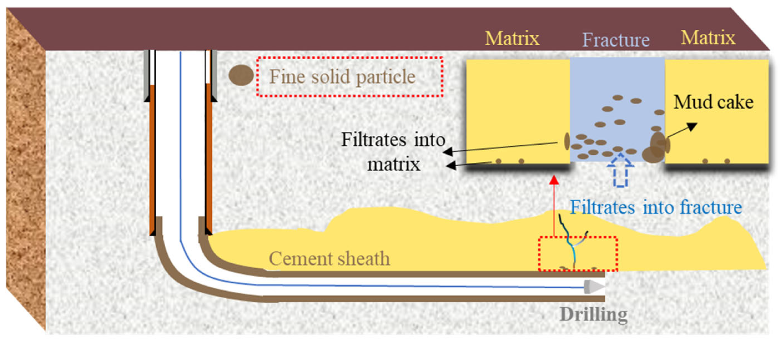
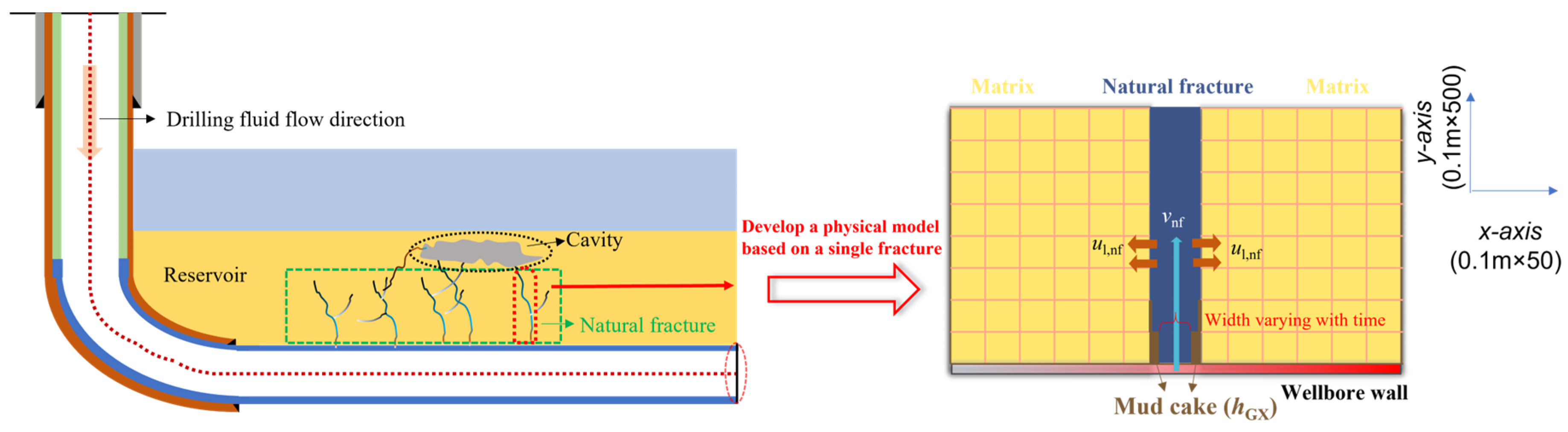
Drilling fluid invasion involves multi-scale coupled flow: filtrate leaks from the fracture into the surrounding matrix under the imposed pressure difference, while solid particles are transported with the filtrate. Larger particles accumulate on fracture walls to form a mud cake; fine particles penetrate the matrix, clogging pore spaces and reducing permeability (Figure 3). The combined effects of external mud cake growth and internal pore blockage significantly hinder further filtrate movement.

To describe the above process, this study presents a 2D planar drilling fluid loss model based on the Reynolds equation [26]. The model incorporates non-Newtonian rheological properties [27]. The simulation domain is defined as a rectangular matrix block containing a central natural fracture (Figure 4), with the x-axis representing the wellbore direction and the y-axis the fracture length. The model is based on the following assumptions:

• The rock matrix is treated as an isotropic, homogeneous medium.
• The influence of gravity on fluid flow is neglected.
• Natural fractures are oriented perpendicular to the wellbore axis, their height is equal to the reservoir thickness, and they do not propagate during the drilling fluid contamination process.
• The pore space is considered incompressible, while the fluid is slightly compressible.

2.3.2. Governing Equations

(1) Fluid flow equations

The model is divided into a matrix domain and a fracture domain. In the matrix domain, the governing equation for flow within the porous matrix medium is given by Equation (1):

$$\rho {\displaystyle \frac{\partial }{\partial x}}\left({\displaystyle \frac{k_{\mathfrak{m}}}{\mu }}{\displaystyle \frac{\partial p_{\mathfrak{m}}}{\partial x}}\right)+\rho {\displaystyle \frac{\partial }{\partial y}}\left({\displaystyle \frac{k_{\mathfrak{m}}}{\mu }}{\displaystyle \frac{\partial p_{\mathfrak{m}}}{\partial y}}\right)=\rho \varphi C_{\mathrm{t}}{\displaystyle \frac{\partial p_{\mathfrak{m}}}{\partial t}}$$

(1)

In the fracture domain, the material balance equation governing drilling fluid flow within the natural fracture is given by Equation (2):

$${\displaystyle \frac{\partial \left(w_{\mathrm{nf}}{v}_{\mathrm{nf}}\right)}{\partial y}}+u_{\mathrm{l},\mathrm{nf}}=-{\displaystyle \frac{\partial w_{\mathrm{nf}}}{\partial t}}$$

(2)

Based on the local cubic law, the flow velocity within natural fractures is calculated using Equation (3):

$$v_{\mathrm{nf}}={\displaystyle \frac{w_{\mathrm{nf}}^2}{12\mu }}{\displaystyle \frac{\partial p_{\mathrm{nf}}}{\partial \mathrm{y}}}$$

(3)

Substituting Equation (3) into Equation (2) yields the governing equation for fluid flow within the fracture, presented as Equation (4):

$${\displaystyle \frac{\partial }{\partial y}}\left({\displaystyle \frac{w_{\mathrm{nf}}^3}{12\mu }}{\displaystyle \frac{\partial p_{\mathrm{nf}}}{\partial y}}\right)+u_{1,\mathrm{nf}}=-{\displaystyle \frac{\partial w_{\mathrm{nf}}}{\partial t}}$$

(4)

where u_l.nf is calculated using Darcy’s law, presented as Equation (5):

$$u_{\mathrm{l},\mathrm{nf}}={\displaystyle \frac{k_{\mathrm{W}}}{\mu }}{\displaystyle \frac{p_{\mathrm{nf}}-p_{\mathrm{m}}}{\raisebox{1ex}{$w_{\mathrm{nf}}$}\!\left/ \!\raisebox{-1ex}{$2$}\right.}}$$

(5)

$$k_{\mathrm{W}}={\displaystyle \frac{k_{\mathrm{m}}{k}_{\mathrm{mc}}\left(\Delta x+h_{\mathrm{mc}}\right)}{\Delta x{k}_{\mathrm{mc}}+h_{\mathrm{mc}}{k}_{\mathrm{m}}}}$$

(6)

(2) Drilling fluid solid phase concentration equation

The concentration distribution of the drilling fluid’s solid phase is determined by solving a convective mass transfer equation, which accounts only for the migration of solid particles carried by the drilling fluid without considering diffusive effects. In this context, the transport of the solid phase within the natural fracture is governed by Equation (7):

$${\displaystyle \frac{\partial C_{\mathrm{D}}}{\partial t}}+v_{\mathrm{nf}}{\displaystyle \frac{\partial C_{\mathrm{D}}}{\partial y}}=0$$

(7)

(3) Natural fracture width evolution equation

During the process of drilling fluid filtration into the matrix, solid particles unable to penetrate the matrix pore throats accumulate on the rock fracture surfaces, forming a mud cake. The total solid mass that migrates with the drilling fluid into the matrix is calculated by Equation (8):

$$M_{\mathrm{D}}=C_{\mathrm{D}}{u}_{\mathrm{l},\mathrm{nf}}\Delta yh\Delta t$$

(8)

The mud cake is composed of tightly packed solid particles that are unable to enter the matrix, and its thickness is calculated by Equation (9):

$$h_{\mathrm{mc}}={\displaystyle \frac{M_{\mathrm{D}}\left(1-f_{\mathrm{D}}\right)}{h\Delta y{\rho }_{\mathrm{D}}}}$$

(9)

The natural fracture width after mud cake formation is calculated by Equation (10):

$$w_{\mathrm{nf}}=w_{\mathrm{ini}}-2h_{\mathrm{mc}}$$

(10)

(4) Matrix permeability evolution equation

Fine solid particles that are capable of entering the rock matrix occupy pore spaces, leading to a reduction in porosity (Equation (11)):

$${\varphi }^{\prime }={\displaystyle \frac{V_{\mathrm{p}}-\frac{C_{\mathrm{D}}{u}_{\mathrm{l},\mathrm{nf}}\mathsf{\Delta }yh\left(1-f_{\mathrm{D}}\right)}{{\rho }_{\mathrm{D}}}}{V_{\mathrm{total}}}}$$

(11)

Subsequently, the matrix permeability after contamination is calculated by Equation (12):

$$k_{\mathrm{m}}^{\prime }=k_{re}{\displaystyle \frac{{\varphi }^{\prime }}{{\varphi }_{re}}}{\left({\displaystyle \frac{{\varphi }^{\prime }\left(1-{\varphi }_{re}\right)}{{\varphi }_{re}\left(1-{\varphi }^{\prime }\right)}}\right)}^{2\beta }$$

(12)

2.3.3. Model Solution

Initial conditions: at t = 0, the natural fracture width is specified, and drilling fluid has not yet flowed through the fracture channel, resulting in a drilling fluid concentration of zero within the fracture (Equation (13)).

$$w_{\mathrm{nf}}=w_{\mathrm{ini}},C_{\mathrm{nf}}=0t=0$$

(13)

The bottomhole pressure is applied at the inlet, the reservoir pressure is applied at the outlet, and closed boundaries are defined on the left and right sides (Equation (14)).

$$\left\{\begin{array}{l}P=P_{\mathrm{wf}} 0\le x\le L_x,y=0\\ P=P_{\mathrm{res}} 0\le x\le L_x,y=L_y\\ \partial P/\partial x=0 x=0,0\le y\le L_y\\ \partial P/\partial x=0 x=L_x,0\le y\le L_y\\ C_{\mathrm{nf}}=C_0 x=\mathrm{fracture} \mathrm{location},y=0\\ \partial C_{\mathrm{nf}}/\partial y=0 x=\mathrm{fracture} \mathrm{location},y=0\end{array}\right.$$

(14)

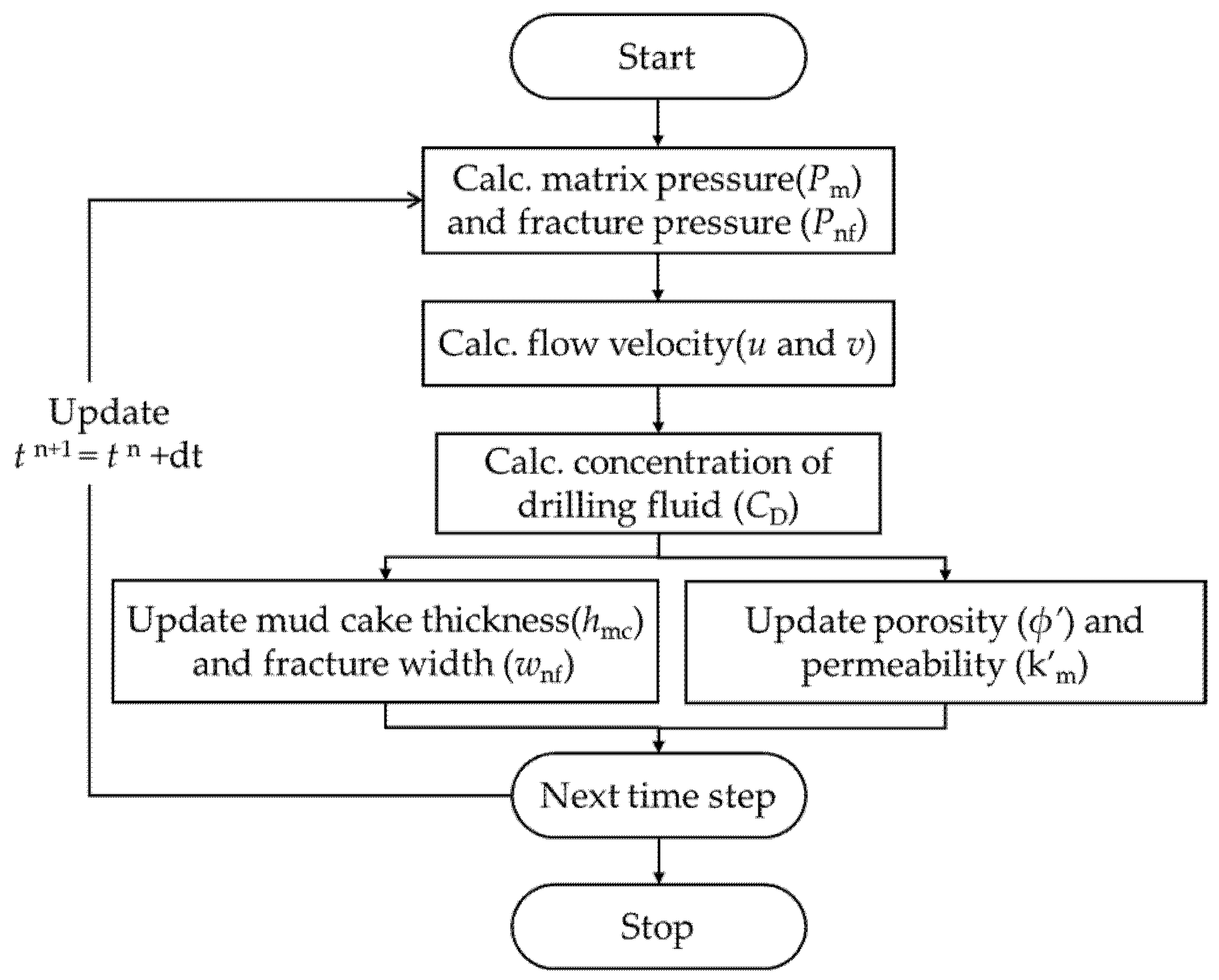
The pressure and concentration fields are solved implicitly, while the mud cake thickness, fracture width and permeability are updated explicitly via Equations (8)–(12) at each time step.

The model solves for the velocity and fracture width of the first grid cell, from which the loss volume is subsequently derived (Equation (15)).

$$V_{\mathrm{loss}}={\displaystyle \sum _{t=0}^{t_{end}}{v}_{\mathrm{nf},1}(t)w_{\mathrm{nf},1}^{\prime }(t)h\Delta t}$$

(15)

The governing equations were implemented in MATLAB (R2023a) using a cell-centered finite volume scheme on a structured grid. The detailed solution procedure is presented as a flowchart in Figure 5.

2.4. An Integrated Approach to Downhole Fracture Interpretation

To reduce the inaccuracy of predicting natural fracture width solely from resistivity logging data in the Shunbei Field, we revised the coefficients in the resistivity-based width calculation formula. Using loss volumes validated by our simulation model, the calculated values agreed well with field observations. A site-specific correlation was then established from collected field fluid loss data. For individual wells, fracture characterization proceeds as follows: well logs are first used to identify fracture locations and numbers based on each fracture’s reservoir contribution (storage and flow capacity). Then, the width of high-angle fractures is calculated using the revised formula.

Furthermore, assuming that all downhole natural fractures exhibiting high storage and permeability significance are high-angle fractures, Equation (16) is employed to calculate the in situ natural fracture width based on well log data [28]:

$$W=A\left(C_{\mathrm{lls}}-C_{\mathrm{lld}}\right)/(4\times {10}^7{R}_{\mathrm{m}})$$

(16)

The methodology described above was applied to well A3 to analyze its natural fracture characteristics. An illustrative example of the procedure is outlined below:

• Based on daily mud logging reports and lost circulation records, the fluid loss intervals for well A3 were identified at depths of 7894.1 m, 7986.68 m, and 8084.78 m.
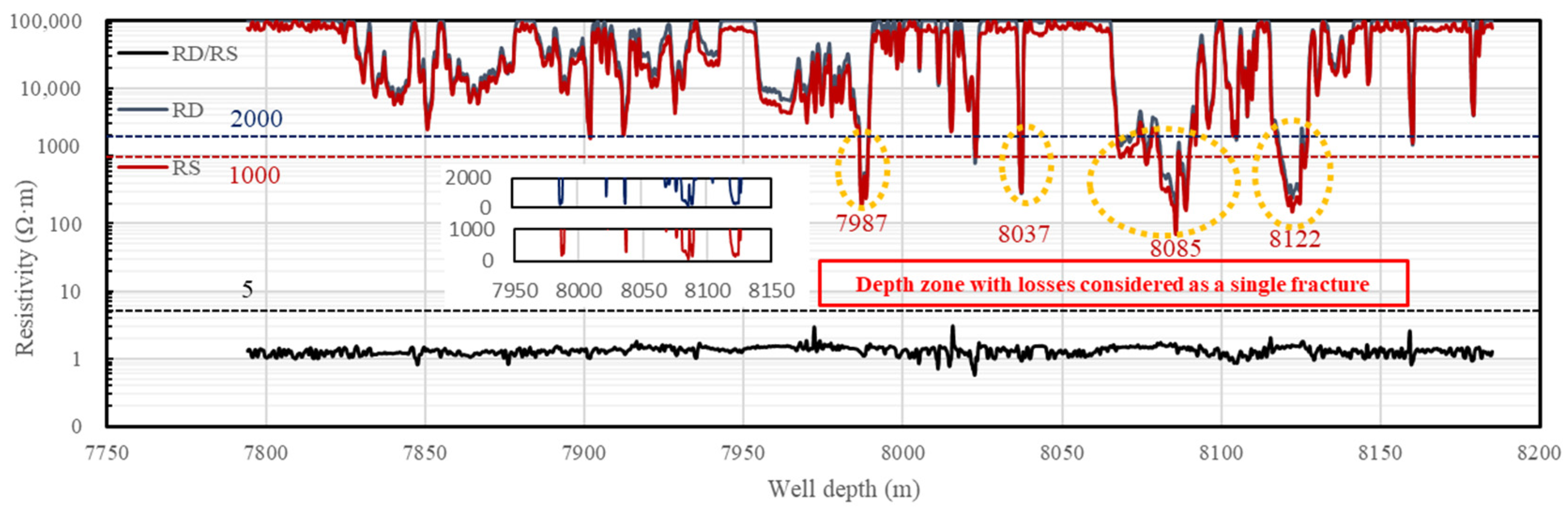
• Utilizing the interpretation criteria based on the RD/RS ratio, RD, and RS values (

  Table 3. Interpretation criteria for fracture significance and extent using deep and shallow laterolog resistivity.

  Fracture Radial Extent	Reservoir Significance	Formation Type	Resistivity (Ω·m)		Ratio
  			Deep Laterolog (RD)	Shallow Laterolog (RS)	RD/RS
  <0.5 m (often indicates induced fractures)	Negligible significance	Low-porosity limestone	>8000	<3000	<5
  		Limestone with effective porosity	>8000	>1000
  0.5–2.5 m (apparent natural fractures)	Negligible significance	Low-porosity limestone	8000~2000	<3000	5~11
  		Limestone with effective porosity	<1000	<1000
  >2.5 m (significant natural fractures)	Some significance	Low-porosity limestone	<2000	<1000	<5
  		Limestone with effective porosity	<1000	<500

  ), we identified the intervals with significant storage and permeability (reservoir significance) for well A3 at depths of 7987 m, 8037 m, 8085 m, and 8122 m (Figure 6). These depths exhibited a good correspondence with the identified fluid loss intervals.

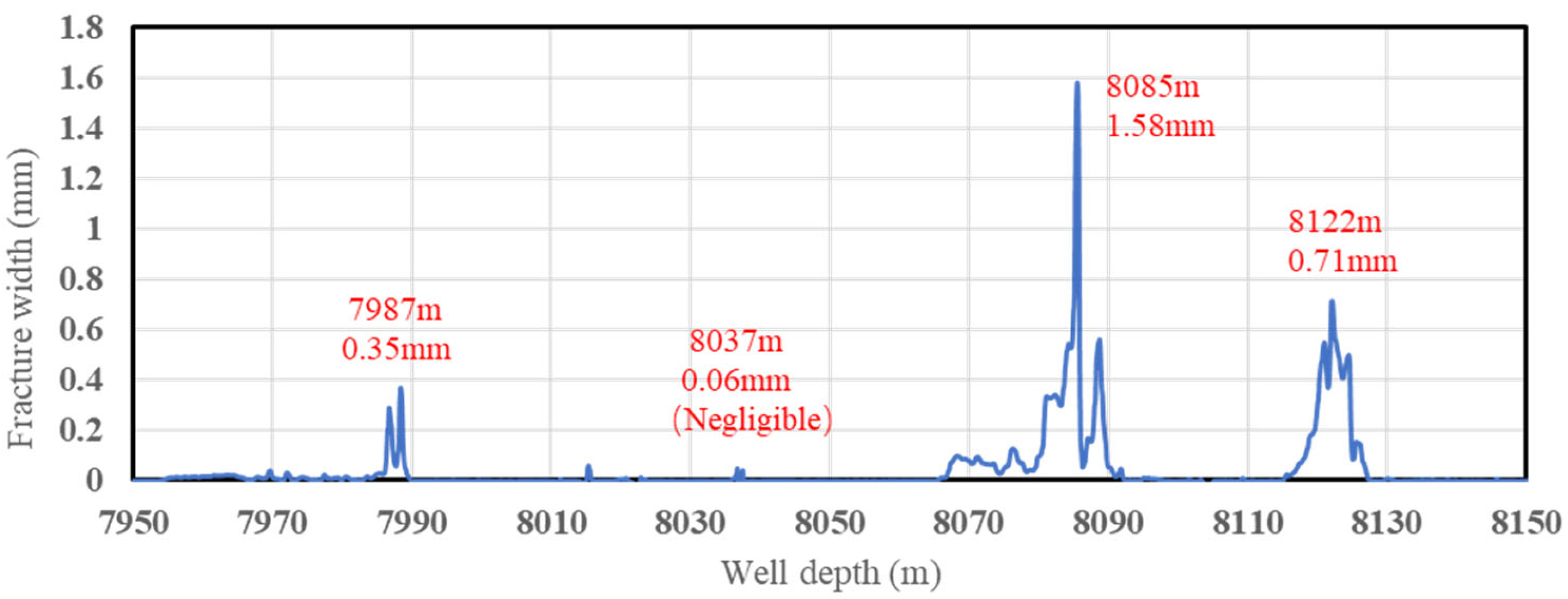
• Using the formula for high-angle fracture width (Equation 16), the corresponding fracture widths were calculated as 0.35 mm, 0.06 mm, 1.58 mm, and 0.71 mm, for the depths identified in the second step.
• Based on the width–loss volume relationship, the 0.06 mm wide fracture was considered to contribute negligible fluid loss (Figure 7). Consequently, the effective number of contributing fractures for fluid loss calculations was determined to be 3.

3. Results

3.1. Drilling Fluid Damage Test Results

3.1.1. Solid Phase Particle Size Distribution Test

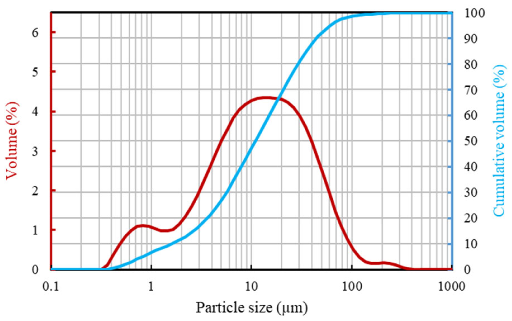
Experimental results indicate that the solid particles in the drilling fluid range in size from 0.3 μm to 416.9 μm, with an average particle size of 19.2 μm. As shown in Figure 8, the particle size distribution exhibits a trimodal pattern, where particles in the 1–100 μm size range constitute the predominant fraction (92.4%). The volume fraction of larger particles (>100 μm) is relatively small (1.3%).

Utilizing the Kozeny Equation [29] applied to core casting thin section analysis (Figure 8), we determined the average pore-throat diameter to be 5.2 μm.

$$d={(180k_{\mathrm{c}}{(1-{\phi }_{\mathrm{c}})}^2/{\phi }_{\mathrm{c}}^3)}^{0.5}$$

(17)

According to Abrams’ rule [30], particles smaller than one-third of the pore-throat diameter (<1.7 μm) are too small to bridge and therefore invade the matrix. As summarized in

Table 4. Solid phase invasion ratio based on reservoir parameters and drilling fluid density.

Porosity (%)	Average Pore Throat Diameter (μm)	Upper Size Limit of Invading Particles (μm)	Solid Phase Invasion (%)	Mud Cake Proportion (%)
2~3	5.2	1.7	10	90

, the fraction of solid particles below 1.7 μm is 10%.

3.1.2. Laboratory-Based Characterization of Drilling Fluid Damage

Table 5. Experimental results for drilling fluid flooding in fractured cores.

No.	Initial Permeability (md)	Equivalent Width (μm)	Drilling Fluid Lost Volume (ml)	Permeability After Flooding (md)	Damage Rate (%)
1	27	18	0.95	0.04	99
2	234	53	4.2	148	37
3	1452	132	16	210	85
4	1976	154	14	909	54
5	2821	184	19	1818	36
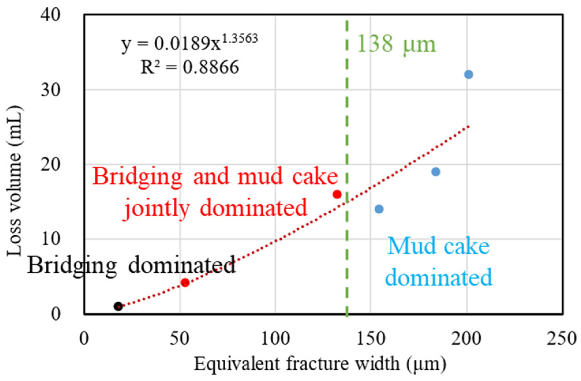
6	3366	201	32	931	72

summarizes the drilling fluid flooding experiments on fractured core samples. Plugging was achieved under all conditions. The lost volume increases with initial fracture width, following a clear power-law relationship (Figure 9). In narrow fractures, mud cakes and bridging form quickly, leading to plugging and limiting fluid loss. As fracture width increases, bridging becomes more difficult, causing a rise in lost volume. Specifically, particles smaller than 46 μm account for over 90% of the solid volume (Figure 8). Therefore, when the fracture width exceeds three times this value (>138 μm), the probability of effective bridging decreases according to Abrams’ rule. However, experiments show that even for fracture widths ≥ 132 μm, plugging still occurs and the power-law relationship still holds. This indicates that mud cake formation on fracture walls also plays a key role in controlling fluid loss in fractured reservoirs.

However, no clear correlation was observed between damage rate and fracture width. While the underlying cause remains to be confirmed, one possible explanation is the stochastic and non-uniform nature of solid plugging. Another is that partial damage removal may have occurred during the reverse core-flooding tests. Except for the 18 μm fracture, which was completely plugged (damage rate 99%), overall damage rates ranged from 36% to 85%.

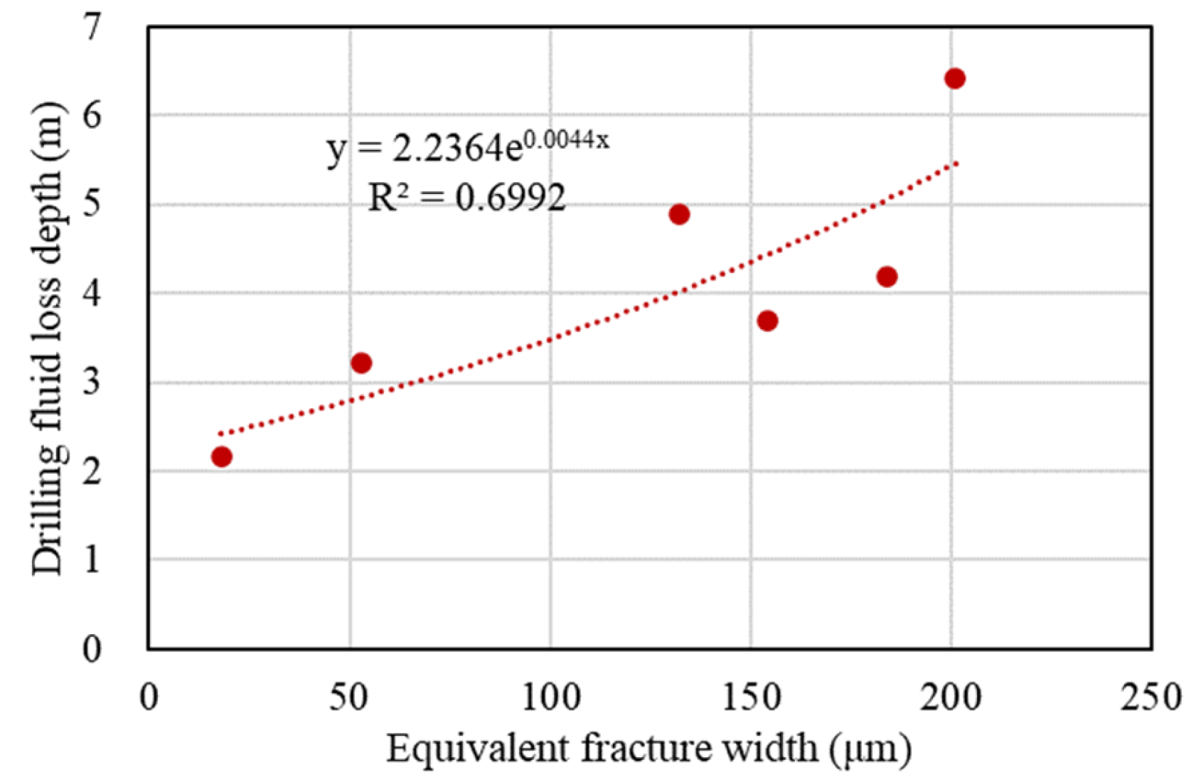
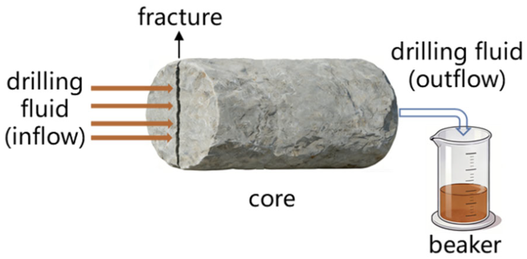
As illustrated in Figure 10, the fracture cross-sectional area is approximated as the product of the equivalent fracture width and the core diameter. Subsequently, based on the volume of drilling fluid discharged at the outlet, the predicted drilling fluid loss depth is calculated by Equation (18):

$$L_{\mathrm{loss}}= V_{\mathrm{out}}/\left(w_{\mathrm{c}}{d}_{\mathrm{c}}\right)+L_{\mathrm{c}}$$

(18)

As shown in Figure 11, for fracture widths ranging from 18 to 201 μm, the predicted drilling fluid loss depth is between 2.16 and 6.42 m. Overall, the predicted loss depth exhibits an exponential relationship with fracture width (R² = 0.69).

3.2. Drilling Fluid Contamination Simulation

The initial parameters used for the simulation are listed in

Table 6. Model parameters.

Category	Parameter	Value	Source
Engineering parameters	Drilling time (min/m)	15	Field data
	Drilling pressure differential (MPa)	7
Geological parameters	Depth (m)	7600
	Pressure coefficient (dimensionless)	1.13
	Matrix porosity (%)	2	Laboratory data
	Natural fracture width (μm)	100~300 (in 50 increments), 500, 1000, 2000, 5000, 10,000
Drilling fluid parameters	Drilling fluid density (g/cm3)	1.5
	Mud cake permeability (md)	10−5

. Based on the H-B rheological model and the definition of apparent viscosity, the rheological properties of the drilling fluid conform to the H-B model, as described in Equation (19).

$$\mu =10592.2\cdot {\gamma }^{-1}+86.17\cdot {\gamma }^{-0.0921}$$

(19)

Given that the solid particle size of the drilling fluid is primarily on the order of 100 μm, fracture widths of 100–300 μm were selected based on the one-third bridging principle to investigate plugging mechanisms. Meanwhile, to investigate the mechanism of lost circulation in large millimeter-scale fractures under field conditions, fracture widths of 500–10,000 μm were also set in this study.

3.2.1. Model Validation

To validate the model, parameters were set to match the experimental conditions (Table 2). The loss volume was calculated using Equation (15), and the loss depth was determined based on the same loss depth definition used in the experiments (Equation (20)).

$$L_{\mathrm{loss}}^{\prime }=V_{\mathrm{loss}}/w_{\mathrm{nf},1}/h$$

(20)

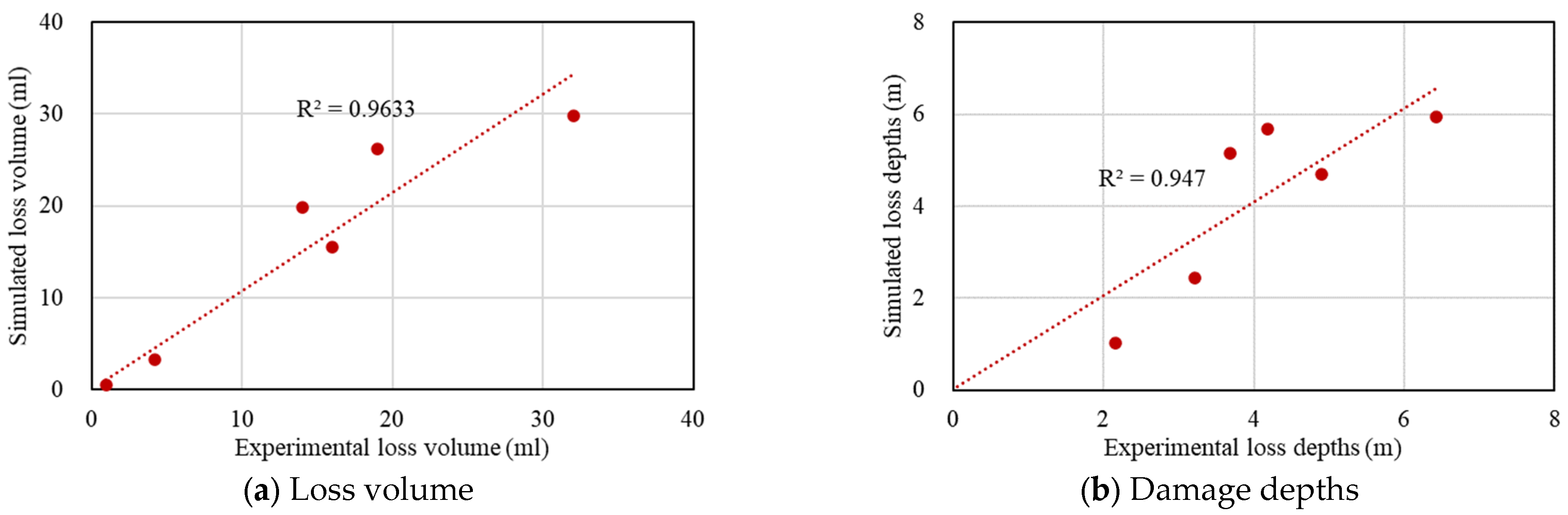
As shown in Figure 12, the simulated loss volumes agreed closely with the experimental measurements, yielding R² = 0.963, RMSE = 3.37 mL, and MAE = 2.91 mL. Similarly, the simulated loss depth showed good agreement, with R² = 0.947, RMSE = 1.04 m, and MAE = 0.96 m. These results confirm the reliability of the developed model.

3.2.2. Mechanism of Mud Cake Growth and Damage

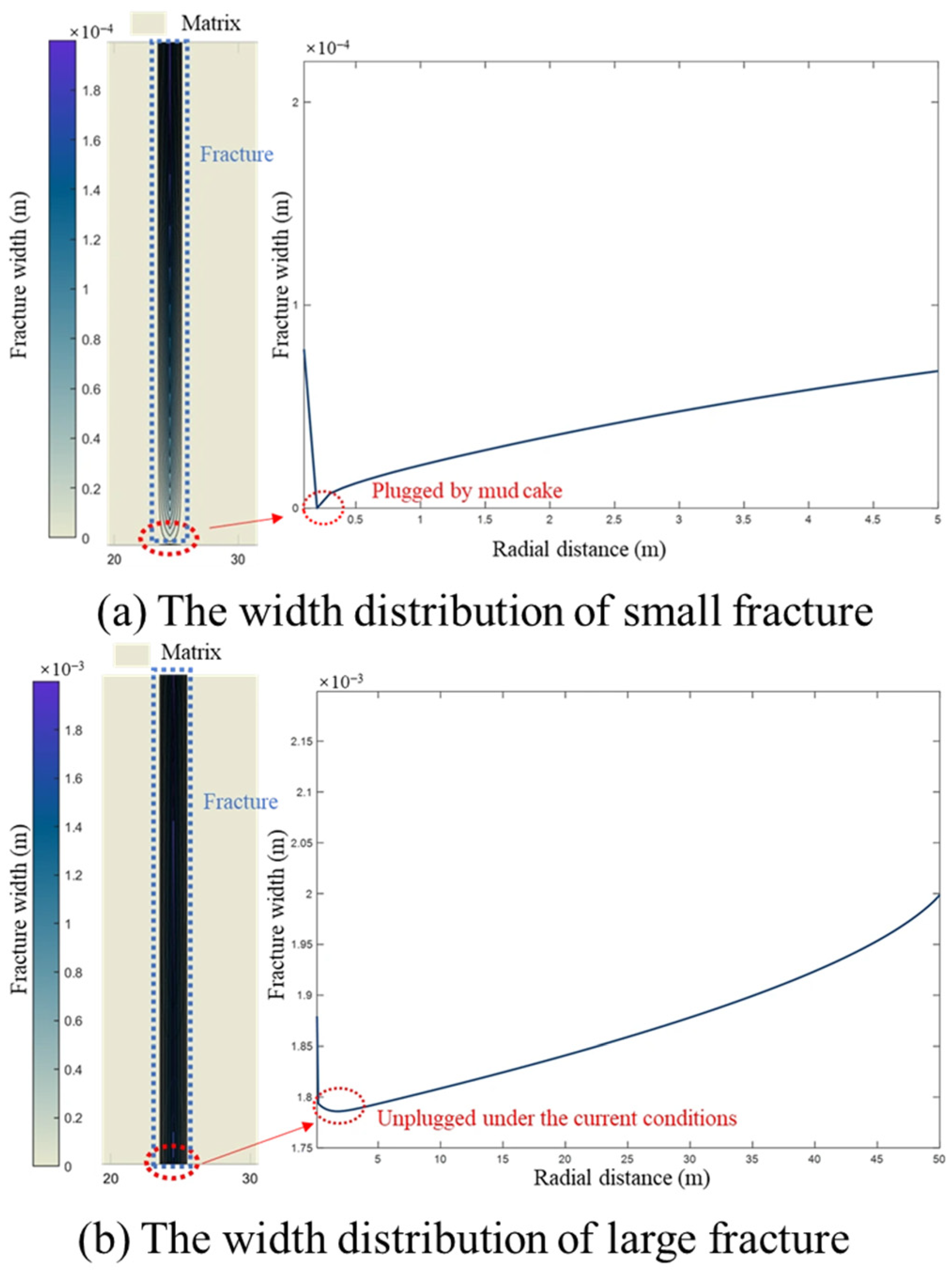
Simulation results showed that the mechanisms of mud cake growth differ between fractures with widths of 100–300 μm and those with widths of 500–10,000 μm. Based on field observations from the Shunbei Block, fracture widths of 200 μm and 2000 μm were selected as representative cases for small and large fractures, respectively.

As shown in Figure 13a, a dense mud cake completely plugs the small fracture within 0.2 m of the wellbore wall. The minimum width does not occur at the first grid cell adjacent to the wellbore but at a farther location, due to the filtration behavior at the fracture entrance. The entrance grid cell receives filtrate from two sources: wellbore-to-matrix invasion and fracture-to-matrix leak-off. Particles from the wellbore do not contribute to mud cake; instead, they raise local pressure, reducing leak-off from the fracture face and inhibiting mud cake growth at the mouth. Thus, initial plugging occurs away from the wellbore.

As illustrated in Figure 13b, the large fracture did not become completely plugged under the current conditions. The minimum width appears at 1.7 m from the wellbore, and with longer invasion, plugging would likely occur at or beyond this point. Unlike small fractures, the width profile along the large fracture is convex with increasing distance from the wellbore, due to greater fluid loss into deeper formations. Consequently, the mud cake grows slowly, making effective plugging more difficult.

3.2.3. The Effect of Width on Mud Cake Growth Evolution and Fluid Loss Dynamics

Simulations were conducted with fracture widths ranging from 100 μm to 300 μm (small fractures) and 500 μm to 10,000 μm (large fractures) to analyze fluid loss mechanisms.

(1) Mud cake growth evolution

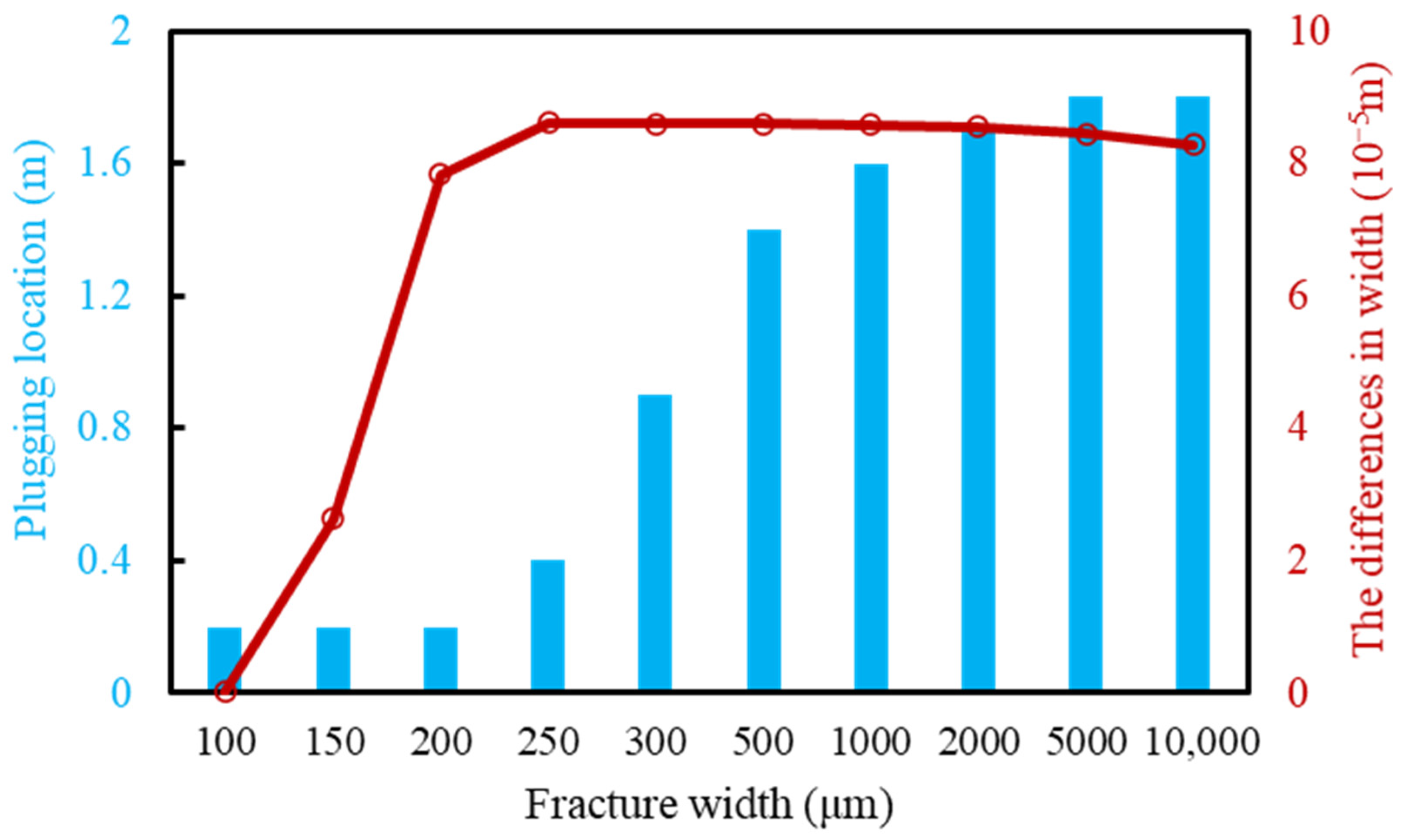
The location of the minimum fracture width after contamination was used as the representative plugging location, and the width difference between the first and second grid cells was statistically analyzed (Figure 14).

Overall, the plugging location moved farther from the wellbore as the initial fracture width increased, primarily governed by mud cake growth dynamics. Fluid loss from the wellbore into the matrix inhibited mud cake development. Because mud cake grew more slowly in wider fractures, bridging took longer, allowing the zone of matrix-to-matrix flow to extend further. The plateau observed at the largest widths represented the physical limit of wellbore-to-matrix invasion under the current conditions.

In fractures narrower than 200 μm, the width difference between the first and second grid cells increased with fracture width, as complete plugging was achieved. After plugging, the sharp permeability reduction halted fluid flow, causing rapid pressure buildup and reduced fluid loss. Thus, mud cake formation constricted the fracture more effectively in narrower fractures. In larger, unplugged fractures, this width difference gradually decreased as fracture width increased, because the influence of wellbore-to-matrix fluid loss diminished with width.

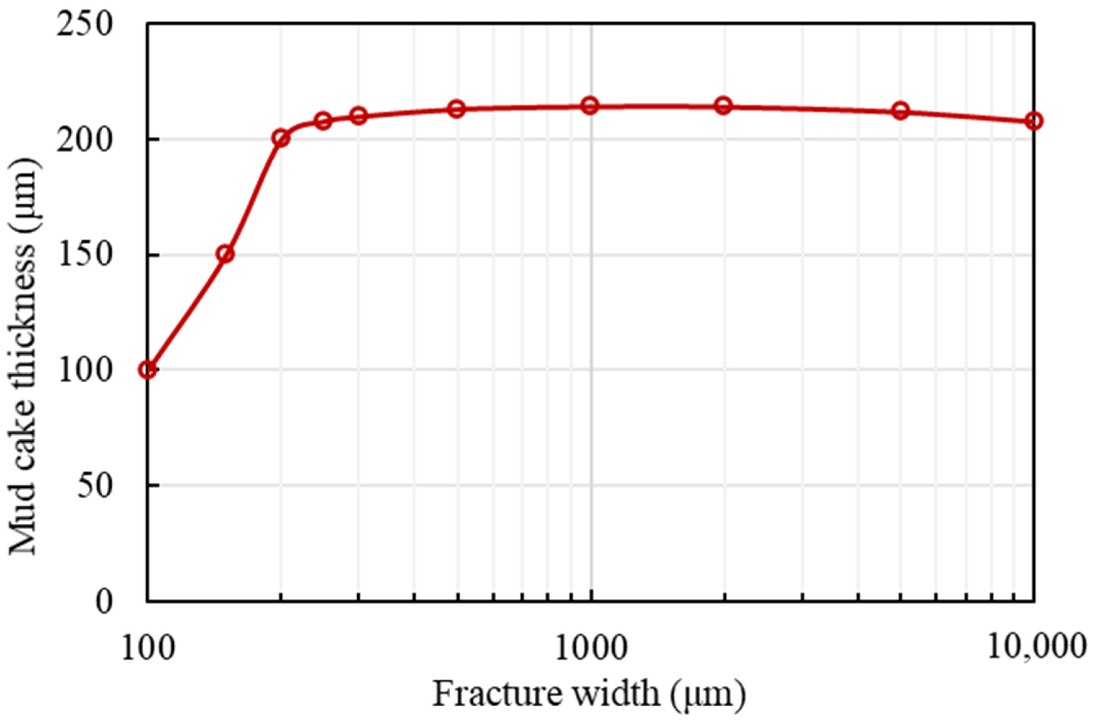
Figure 15 further illustrates the evolution of mud cake thickness with fracture width. Overall, the mud cake thickness exhibits a non-monotonic trend, first increasing and then decreasing as fracture width increases. In small fractures, the mud cake thickness increases with fracture width, as the limited width restricts both the invasion rate and the available space for mud cake growth, promoting particle accumulation and the formation of a dense sealing layer near the wellbore. In large fractures, the mud cake thickness begins to decline. This is attributed to the higher fluid invasion velocity in wider fractures, which transports the mud cake particles deeper into the fracture before an effective plug can be established, thereby thinning the cake at the plugging point. These observations indicate that, under the conditions of this study, the sealing capacity of mud cake alone is limited. While self-plugging by mud cake is sufficient in small fractures, wider fractures require additional engineering measures (e.g., bridging agents or particle-size optimization) to achieve effective loss control.

(2) Fluid loss behavior

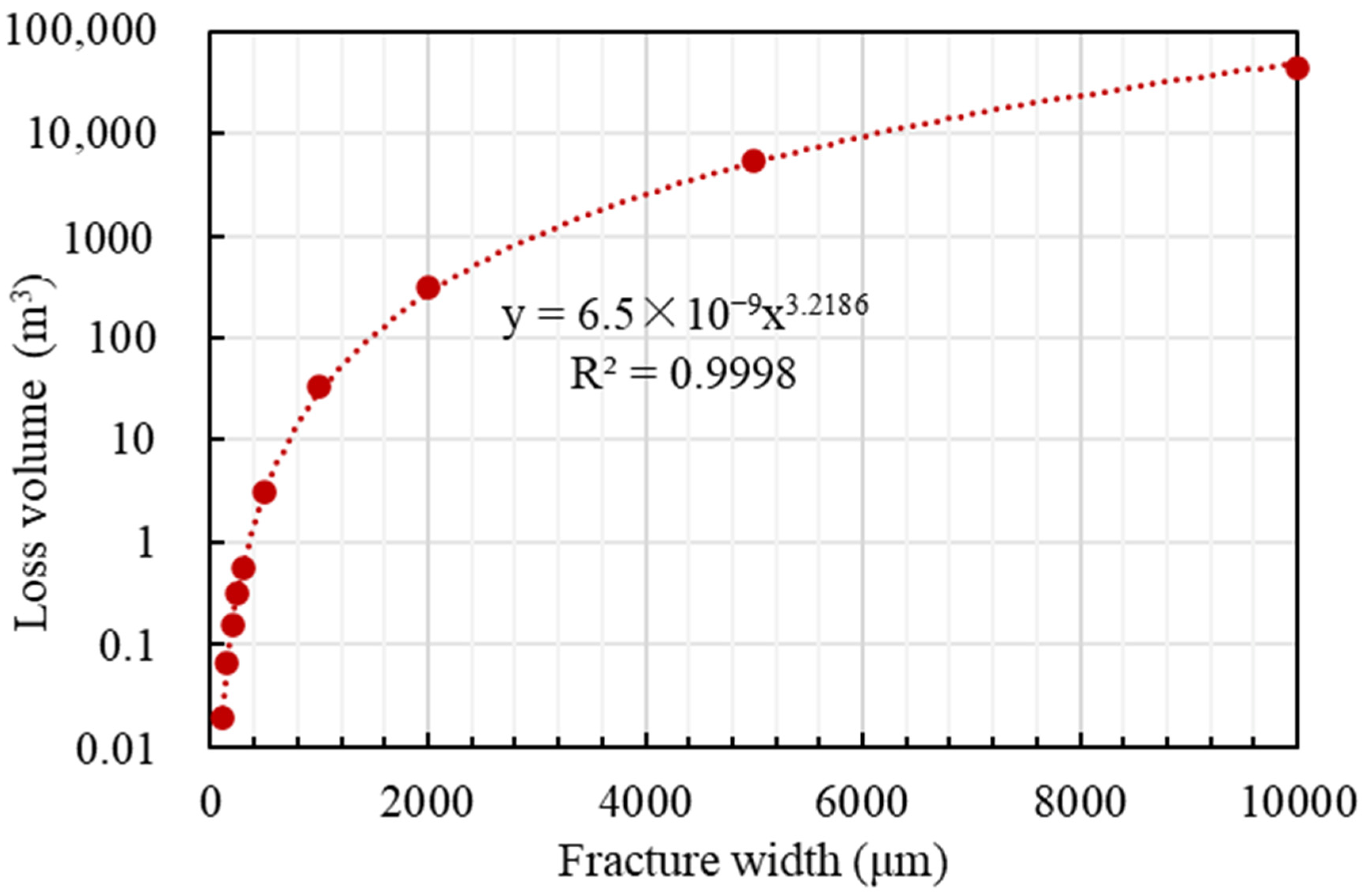
As shown in Figure 16, the cumulative loss volume exhibited a strong power-law relationship with fracture width (R² > 0.99), consistent with experimental observations. A wider flow channel delayed plugging and prolonged fluid loss, increasing total loss volume. Once the fracture width exceeded 200 μm, effective mud cake plugging failed, and loss volume rose sharply as the contribution of plugging diminished.

3.3. Field Application of the Integrated Interpretation Method

As described in Section 2.4 above, the correction of coefficient (A) was completed using the width–loss volume relationship (Figure 16). For different values of the coefficient (A), the number of fractures, fracture widths (W), and corresponding loss volumes were determined for various well intervals using well log data. Using wells A3 and A7 as examples, the coefficients were calibrated for the Shunbei Block (

Table 7. Comparison of results using different correction coefficients for well A3 and A7.

Well	Fracture Count	Log-Interpreted Fracture Width (mm)	Formula Coefficient (A)	Total Fracture Width (mm)	Loss Volume (m3)	Total Loss Volume (m3)	Field Loss Volume (m3)
A3	3	1.6	3	4.8	4242	5302	6625
		0.4		1.2	259
		0.7		2.1	801
		1.6	4.3	6.9	8763	10,955
		0.4		1.7	536
		0.7		3	1656
		1.6	3.15	5	5442	6840
		0.4		1.3	346
		0.7		2.2	1052
A7	1	4.5	1	4.5	3724	3724	3285
		1.2	4.3	5.16	4907	4907
		1.2	3.15	3.78	3072	3072

Note: The total fracture width is the sum of the widths of all contributing fractures in a well.

). The relative error in the calculated loss volume was minimized when A = 3.15, yielding relative error values of 0.06 and 0.03, respectively. This indicates a good match between the revised formula results and actual field measurements.

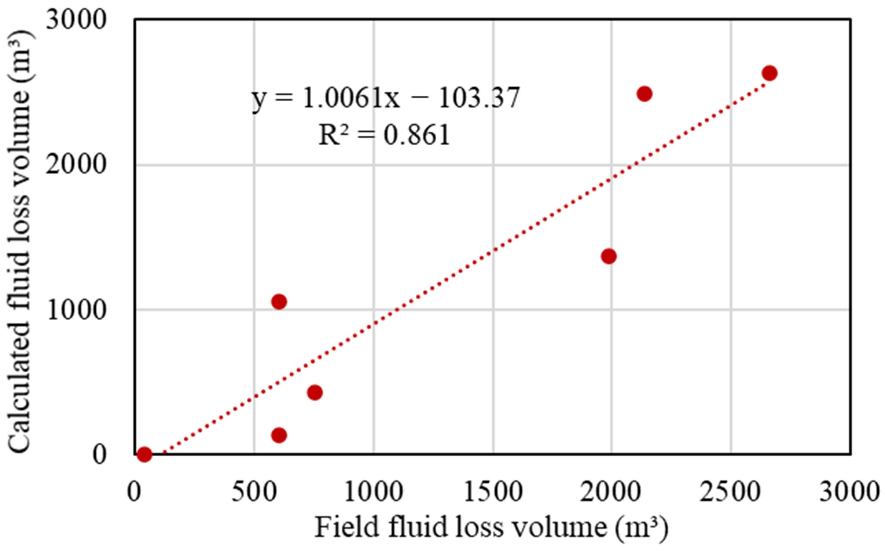
With A = 3.15, the calculated loss volumes agreed well with the field measurements (R² = 0.86), as presented in

Table 8. Comparison between calculated (post-calibration) and field loss volumes.

Well	Single-Fracture Assumption		Multi-Fracture Calibration Using Well-Log Data
	Fracture Width (mm)	Loss Volume (m3)	Number of Fractures (Dimensionless)	Fracture Width (mm)	Loss Volume (m3)	Total Loss Volume (m3)
A1	0.9	39	1	0.15	5.56	5.56
A2	2.1	756	2	1.26	346	433
				0.63	87
A3	6.2	6625	3	5.04	5442	6840
				1.26	346
				2.21	1052
A4	2.8	2138	2	3.15	2138	2484
				1.26	346
A5	2.7	1985	1	2.52	1372	1372
A6	2.9	2666	3	2.84	1734	2630
				1.51	497
				1.35	399
A7	3.6	3285	1	3.78	3072	3072
A8	2	605	1	2.2	1052	1052
A9	2.1	609	1	0.78	136	136

Note: Under the single-fracture assumption, total loss volume is assigned to one equivalent fracture and its width is back-calculated from Figure 16; under multi-fracture calibration, the loss volumes from all logged fractures are summed.

and Figure 17. This demonstrates the reliability of the fracture widths and counts derived from the well log data using the adjusted formula.

4. Discussion

The plugging of a natural fracture depends on the balance between coarse-particle bridging and mud-cake growth on the fracture walls. The 138 μm threshold identified in this study reflects the transition from particle-bridging dominance to mud-cake sealing dominance. While Abrams’ one-third rule [30] predicts bridging failure above ~132 μm, laboratory data confirm that complete plugging can still be attained for widths up to 201 μm, attributed to sealing by mud-cake growth. This observation extends the findings of Ezeakacha and Salehi [23], who demonstrated mud-cake-controlled filtration in porous carbonates, to the context of natural fractures. Notably, the sealing mechanism shifts within a narrow window (138–200 μm). Beyond 200 μm, neither mechanism is sufficient to seal the fracture. This trend is corroborated by the experimental findings of You et al. [31], who reported a critical bridging threshold of approximately 150 μm and observed that mud-cake sealing efficiency decreases substantially in the 200–300 μm range. Although differences in experimental samples exist, these findings provide a degree of support for the results of the present study.

The calibrated coefficient A = 3.15 systematically corrects the resistivity-based underestimation of fracture aperture [28], which is consistent with the known limitation of laterolog-based estimates in intervals invaded by mud filtrate. In the multi-fracture interpretation, each contributing fracture is treated as an independent conduit, an assumption that is widely accepted when the fracture network is not highly dense [32]. The close match between the interpreted parameters and the field loss data lends strong support to this assumption. Consequently, the overall self-consistency of the interpretation validates the proposed integrated approach and confirms its applicability to the studied interval.

Despite these consistencies, several limitations should be acknowledged. First, the experimental validation of the bridging threshold relies on single core plugs per width condition (n = 1), precluding statistical repeatability. Second, the proposed 138 μm criterion remains a particle-size-based engineering proxy, lacking direct microscopic corroboration (e.g., SEM/CT imaging) of the bridging morphology. Third, the absence of a correlation between damage rate and width is tentatively attributed to stochastic plugging or partial damage removal during reverse flooding, yet this hypothesis requires direct verification. Finally, the model simplifies fracture surface roughness and stress-induced dynamic closure (accounted for only via equivalent cubic-law width and imposed pressure differential), and the independent-fracture assumption may not hold for strongly interconnected fracture networks.

5. Conclusions

This study integrated experiments, a fracture loss model with dynamic mud cake growth, and field data to evaluate drilling fluid damage in fractured carbonate reservoirs. The key novel findings are summarized below:

• Effective bridging plugging became difficult when the fracture width exceeded 138 μm, as the probability of bridging decreased significantly.
• Cumulative loss volume increased rapidly with fracture width. Moreover, the contribution of mud cake growth to plugging diminished as width increased, and effective plugging was no longer achievable for fractures wider than 200 μm.
• A robust framework was established by calibrating resistivity-derived fracture width formulas using experimental, numerical, and field loss data. Validation across 9 wells yielded strong predictive accuracy (R² = 0.86). This framework enables reliable identification of fracture parameters and damage characteristics, supporting lost circulation control in ultra-deep fractured carbonate reservoirs.

Future work will treat the liquid and solid components of the drilling fluid separately within a multiphase transport formulation, couple fracture deformation and roughness with mud-cake growth, and verify the plugging mechanism on a microscale basis.

References

1. Ma, Y.; Cai, X.; Yun, L.; Li, Z.; Li, H.; Deng, S.; Zhao, P. Practice and theoretical and technical progress in exploration and development of Shunbei ultra-deep carbonate oil and gas field, Tarim Basin, NW China. Pet. Explor. Dev. 2022, 49, 1–20. [Google Scholar] [CrossRef] [Scilit]
2. Deng, Z.; Zhou, D.; Dong, H.; Huang, X.; Wei, S.; Kang, Z. Deep learning for predicting porosity in ultra-deep fractured vuggy reservoirs from the Shunbei oilfield in Tarim Basin, China. Sci. Rep. 2024, 14, 29605. [Google Scholar] [CrossRef] [Scilit] [PubMed]
3. Ma, Y.; Cai, X.; Li, M.; Li, H.; Zhu, D.; Qiu, N.; Pang, X.; Zeng, D.; Kang, Z.; Ma, A.; et al. Research advances on the mechanisms of reservoir formation and hydrocarbon accumulation and the oil and gas development methods of deep and ultra-deep marine carbonates. Pet. Explor. Dev. 2024, 51, 795–812. [Google Scholar] [CrossRef] [Scilit]
4. Wang, Z.; Fu, L.; Jian, S.; Deng, W. Application of a model-driven simultaneous prestack inversion of rock physical properties in ultra-deep Ordovician carbonate reservoirs in the Shunbei area. Front. Earth Sci. 2023, 10, 1035735. [Google Scholar] [CrossRef] [Scilit]
5. Aghli, G.; Harami, R.M.; Mohammadian, R. Reservoir heterogeneity and fracture parameter determination using electrical image logs and petrophysical data (a case study, carbonate Asmari Formation, Zagros Basin, SW Iran). Pet. Sci. 2020, 17, 51–69. [Google Scholar] [CrossRef] [Scilit]
6. Bu, X.; Wang, L.; Zhu, L.; Al, E. Characteristics and reservoir accumulation model of Ordovician fault-controlled fractured-vuggy reservoirs in Shunbei oil and gas field, Tarim Basin. Lithol. Reserv. 2023, 35, 152–160. [Google Scholar]
7. Kuang, L.; Liu, H.; Ren, Y.; Luo, K.; Shi, M.; Su, J.; Li, X. Application and development trend of artificial intelligence in petroleum exploration and development. Pet. Explor. Dev. 2021, 48, 1–14. [Google Scholar] [CrossRef] [Scilit]
8. Ozkaya, S.I. Geometry of layer-bound fractures based on fracture density and aperture-depth plots from resistivity image logs of deviated wells. J. Struct. Geol. 2021, 149, 104372. [Google Scholar] [CrossRef] [Scilit]
9. Cao, M.; Feng, H.; Xiao, H. An Improved GAN-Based Image Restoration Method for Imaging Logging Images. Appl. Sci. 2023, 13, 9249. [Google Scholar] [CrossRef] [Scilit]
10. Li, Z.; Zhang, G.; Zhang, X.; Zhang, X.; Long, Y.; Sun, Y.; Lin, C. EILnet: An intelligent model for the segmentation of multiple fracture types in karst carbonate reservoirs using electrical image logs. Nat. Gas. Ind. B 2025, 12, 158–173. [Google Scholar] [CrossRef] [Scilit]
11. Wang, M.; Zhou, Q.; Yin, L.; Dong, Y. Automatic detection and classification of igneous rock fractures from imaging logging using K-mean algorithm and DNN. Front. Earth Sci. 2025, 13, 1640235. [Google Scholar] [CrossRef] [Scilit]
12. Du, L.; Lu, X.; Li, H. Automatic fracture detection from the images of electrical image logs using Mask R-CNN. Fuel 2023, 351, 128992. [Google Scholar] [CrossRef] [Scilit]
13. Li, C.; Zou, C.; Peng, C.; Lan, X.; Zhang, Y. Intelligent identification and segmentation of fractures in images of ultrasonic image logging based on transfer learning. Fuel 2024, 369, 131694. [Google Scholar] [CrossRef] [Scilit]
14. Aghli, G.; Soleimani, B.; Moussavi-Harami, R.; Mohammadian, R. Fractured zones detection using conventional petrophysical logs by differentiation method and its correlation with image logs. J. Petrol. Sci. Eng. 2016, 142, 152–162. [Google Scholar] [CrossRef] [Scilit]
15. Dong, S.; Zeng, L.; Lyu, W.; Xu, C.; Liu, J.; Mao, Z.; Tian, H.; Sun, F. Fracture identification by semi-supervised learning using conventional logs in tight sandstones of Ordos Basin, China. J. Nat. Sci. Eng. 2020, 76, 103131. [Google Scholar] [CrossRef] [Scilit]
16. Zhang, S.; Yan, J.; Cai, J.; Zhu, X.; Hu, Q.; Wang, M.; Geng, B.; Zhong, G. Fracture characteristics and logging identification of lacustrine shale in the Jiyang Depression, Bohai Bay Basin, Eastern China. Mar. Petrol. Geol. 2021, 132, 105192. [Google Scholar] [CrossRef] [Scilit]
17. Sun, J.; Bai, Y.; Cheng, R.; Lyu, K.; Liu, F.; Feng, J.; Lei, S.; Zhang, J.; Hao, H. Research progress and prospect of plugging technologies for fractured formation with severe lost circulation. Pet. Explor. Dev. 2021, 48, 732–743. [Google Scholar] [CrossRef] [Scilit]
18. Ozdemirtas, M.; Babadagli, T.; Kuru, E. Effects of Fractal Fracture Surface Roughness on Borehole Ballooning. Vadose Zone J. 2009, 8, 250–257. [Google Scholar] [CrossRef] [Scilit]
19. Ozdemirtas, M.; Kuru, E.; Babadagli, T. Experimental investigation of borehole ballooning due to flow of non-Newtonian fluids into fractured rocks. Int. J. Rock Mech. Min. 2010, 47, 1200–1206. [Google Scholar] [CrossRef] [Scilit]
20. Jia, L.; Chen, M.; Hou, B.; Sun, Z.; Jin, Y. Drilling fluid loss model and loss dynamic behavior in fractured formations. Pet. Explor. Dev. 2014, 41, 95–101. [Google Scholar] [CrossRef] [Scilit]
21. Li, S.; Kang, Y.; Li, D. Flow model and experimental simulation for leak-off of H-B flow-pattern drilling fluid in fractured formation. Oil Drill. Prod. Technol. 2015, 37, 57–62. [Google Scholar]
22. Dokhani, V.; Ma, Y.; Geng, T.; Li, Z.; Yu, M. Transient analysis of mud loss in fractured formations. J. Pet. Sci. Eng. 2020, 195, 107722. [Google Scholar] [CrossRef] [Scilit]
23. Ezeakacha, C.P.; Salehi, S. An Advanced Coupled Rock–Fluid Computational Model for Dynamic–Radial Mud Filtration with Experimental Validation. Rock Mech. Rock Eng. 2019, 52, 3757–3770. [Google Scholar] [CrossRef] [Scilit]
24. Wang, Z.; Chen, S.; Kong, L. Mechanical Properties and Fracture Propagation in Shale with Different Types of Mineral Cementation: A Case Study of the Longmaxi Formation. Processes 2026, 14, 787. [Google Scholar] [CrossRef] [Scilit]
25. Xu, C.; Yang, X.; Liu, C.; Kang, Y.; Bai, Y.; You, Z. Dynamic fracture width prediction for lost circulation control and formation damage prevention in ultra-deep fractured tight reservoir. Fuel 2022, 307, 121770. [Google Scholar] [CrossRef] [Scilit]
26. Lavrov, A. Newtonian fluid flow from an arbitrarily-oriented fracture into a single sink. Acta Mech. 2006, 186, 55–74. [Google Scholar] [CrossRef] [Scilit]
27. Shahri, M.P.; Mehrabi, M. A new approach in modeling of fracture ballooning in naturally fractured reservoirs. In Proceedings of the Kuwait International Petroleum Conference and Exhibition 2012: People and Innovative Technologies to Unleash Challenging Hydrocarbon Resources, KIPCE 2012, Kuwait City, Kuwait, 10–12 December 2012. [Google Scholar]
28. Zhang, F.; Chen, Y.; Shao, C.; Li, S. Comparison and Improvement of Facture Opening Estimation Model Based on Dual laterolog. Well Logging Technol. 2010, 34, 339–342. [Google Scholar]
29. Carman, P.C. Fluid flow through granular beds. Chem. Eng. Res. Des. 1997, 75, S32–S48. [Google Scholar] [CrossRef] [Scilit]
30. Abrams, A. Mud design to minimize rock impairment due to particle invasion. J. Pet. Technol. 1977, 29, 586–592. [Google Scholar] [CrossRef] [Scilit]
31. You, L.; Zou, J.; Kang, Y.; Bai, R. Mechanisms of Formation Damage by Lost Drilling Fluids in Fractured Tight Metamorphic Rock Gas Reservoirs. Drill. Fluid Complet. Fluid 2024, 41, 719–727. [Google Scholar]
32. Kang, Y.; Xu, C.; You, L.; Yu, H.; Zhang, B. Comprehensive evaluation of formation damage induced by working fluid loss in fractured tight gas reservoir. J. Nat. Gas Sci. Eng. 2014, 18, 353–359. [Google Scholar] [CrossRef] [Scilit]
Figure 1. General flowchart.
Processes 14 02872 g001
Figure 2. Core samples containing natural fractures.
Processes 14 02872 g002
Figure 3. Mud cake growth during the contamination process.
Processes 14 02872 g003
Figure 4. Schematic diagram of the model.
Processes 14 02872 g004
Figure 5. Flowchart of the solution procedure.
Processes 14 02872 g005
Figure 6. Identification of significant permeable downhole fractures.
Processes 14 02872 g006
Figure 7. Calculation of downhole natural fracture width. (Note: Positions with similar well depths are treated as a single fracture, and it is assumed that and individual fractures are assumed not to interact with each other.)
Processes 14 02872 g007
Figure 8. Particle size distribution of the solid phase in the 1.5 g/cm3 drilling fluid. (Red represents volume, and blue represents cumulative volume.)
Processes 14 02872 g008
Figure 9. Variation in loss volume with equivalent fracture width.
Processes 14 02872 g009
Figure 10. Principle of drilling fluid loss depth calculation.
Processes 14 02872 g010
Figure 11. Variation in drilling fluid loss depth with equivalent fracture width.
Processes 14 02872 g011
Figure 12. Comparison of simulated and experimental results.
Processes 14 02872 g012
Figure 13. The width distribution of the fracture after contamination.
Processes 14 02872 g013
Figure 14. Plugging location and grid cell width difference under different fracture widths.
Processes 14 02872 g014
Figure 15. Evolution of mud cake thickness with fracture width. (The mud cake thickness plotted here corresponds to the maximum value along the fracture.)
Processes 14 02872 g015
Figure 16. Variation in loss volume with fracture width.
Processes 14 02872 g016
Figure 17. Comparison between calculated (post-calibration) and field loss volumes (wells A3 and A7 are excluded).
Processes 14 02872 g017