Sensitivity-Based Reference-Time Scaling for Local Orthogonalization of Fractional-Order Model Parameters

Abstract

Fractional-order models are useful for describing systems with memory, anomalous relaxation, and non-classical dynamic behavior. However, parameter estimation in these models may be affected by strong covariance between the kinetic coefficient and the fractional order, reducing the independent interpretability of the estimated parameters. This work proposes a reference-time scaling strategy for an unforced fractional-order decay model and a forced fractional-order step response model, aiming to improve the local conditioning of the estimation problem by making the sensitivity vectors of the dimensionless coefficient and the fractional order locally orthogonal. The covariance structure is analyzed through the local sensitivity matrix, and a sensitivity-based expression for the reference time is derived to set the off-diagonal term of the approximate Gauss–Newton covariance matrix to zero, thereby reducing first-order linear dependencies. The methodology is evaluated using previously reported experimental data from Amiodarone plasma concentration-time profiles for fractional pharmacokinetic modeling and from the temperature response of a didactic thermal system to a step change in the manipulated variable for fractional-order system identification. The results show that the fitted trajectories, residual sums of squares, dimensional kinetic coefficients, and fractional orders remain invariant under reference-time scaling. Nevertheless, the choice of reference time strongly affects the covariance and correlation between the dimensionless parameter $\mu$ or $\kappa$ and $\beta$, while the recovered dimensional coefficients m and k remain invariant. Conventional choices, such as the maximum, arithmetic mean, geometric mean, and harmonic mean of the experimental times, did not systematically reduce parameter correlation. In contrast, the proposed reference time, selected from the local sensitivity structure, reduced the first-order local correlation in both applications. The results indicate that reference-time scaling is a simple reparameterization tool that improves local statistical interpretability under the Gauss–Newton approximation of fractional-order parameter estimates without modifying the physical model or the quality of the fit.

1. Introduction

Fractional-order models represent an important alternative tool for mathematical modeling of systems that exhibit memory, hereditary effects, anomalous relaxation, and distributed transport mechanisms. Applications of fractional calculus include the study of chemical kinetics [1], membrane separation [2], process systems engineering [3], and biological systems [4]. Fractional-order model identification may involve statistical and interpretative challenges that are not always directly addressed by reparameterization strategies originally developed for integer-order models.

Beyond their application to the representation of complex dynamic behavior, fractional-order models have also received increasing attention in system identification and parameter estimation. In these applications, the fractional order must generally be estimated simultaneously with other model coefficients, making the reliability and interpretability of the resulting parameter estimates an important issue. For example, Khan et al. [5] proposed a robust identification strategy for a fractional Hammerstein nonlinear model with impulsive noise and reported its application to a heat exchanger system. All these studies demonstrate that the use of fractional-order models should consider the ability to reproduce non-classical dynamics and also the reliable estimation of the fractional order and the associated model parameters. This provides additional motivation for investigating parameter covariance and reparameterization strategies in fractional-order model identification.

Despite the modeling advantages, the parameter estimation in fractional-order derivative-based models presents important statistical and interpretative challenges. In the linear fractional-order model, dimensional consistency requires the coefficient m to have the physical dimension $\left[m\right]=T^{\beta }$. Similarly, in the fractional kinetic model, the coefficient k has the physical dimension $\left[k\right]=T^{-\beta }$, where the brackets denote physical dimensions and T denotes the dimension of time. Therefore, the model parameter and the fractional order are intrinsically coupled in both the model structure and the dimensional interpretation of the parameters. This coupling may appear as parametric covariance or correlation when both parameters are estimated simultaneously. If this correlation is high, then the model parameter and the fractional order may compensate each other during nonlinear least-squares fitting, making it difficult to distinguish the parameter effects from fractional-order effects.

The importance of parametric covariance is well known in nonlinear parameter estimation. Correlated parameters reduce the independent interpretability of estimates and may lead to elongated confidence regions in parameter space. In kinetic modeling, Schwaab and Pinto [6] addressed this problem for the Arrhenius equation by introducing a reference-temperature reparameterization able to reduce or eliminate parameter correlation. Their work showed that a proper reference value can improve the interpretation of kinetic parameter estimates without changing the fitted physical model. The broader statistical basis of this idea is related to parameter orthogonality, as discussed by Box and Cox [7] and Cox and Reid [8], who showed that suitable parameterizations can reduce cross-information between parameters and improve inferential interpretation.

In fractional models, different studies address parameter estimation, sensitivity, or uncertainty, but the explicit use of reparameterization to control parametric covariance is less common. For example, Friesen et al. [9] reported a parametric analysis of a fractional sorption model using a simplified Hessian matrix to evaluate parameter variance. Guo et al. [10] developed sensitivity functions and sensitivity equations for fractional differential equations, showing that parameter sensitivity is a relevant topic in fractional modeling. Victor et al. [11] addressed simultaneous estimation of the parameters and differentiation order in fractional-order system identification of a thermal system. These works show that sensitivity and uncertainty analysis are present in the fractional-calculus literature; however, their main focus was not the systematic evaluation of how a reference-time scale affects the covariance and correlation between a dimensionless kinetic parameter and the fractional order.

This gap is relevant because a fractional-order model involves a structural interaction between the model parameter and the fractional order, despite a good fit of the model. Therefore, evaluating only the objective function or the estimated value of $\beta$ may be insufficient for rigorous interpretation. A more complete analysis should also investigate the covariance structure of the estimated parameters and determine whether the model parameter effect can be locally separated from the fractional-order effect.

The present work addresses this issue by proposing a reference-time scaling framework for two dimensionless fractional first-order formulations, where the first consists of a fractional decay model and the second describes a forced fractional step response model by applying the methodology originally proposed by Schwaab and Pinto [6] for estimating parameters of the Arrhenius equation. The fractional first-order models are rewritten using a dimensionless time variable and a dimensionless kinetic parameter, and then different reference-time definitions are evaluated, including the maximum experimental time, arithmetic mean, geometric mean, harmonic mean, and a covariance-based reference time. The latter is calculated from the sensitivity structure of the fitted fractional model and is designed to improve the numerical conditioning of the estimation problem by locally orthogonalizing the sensitivity vectors associated with the dimensionless parameters and the fractional order. This considerably reduces the off-diagonal term of the approximate variance-covariance matrix derived from the Gauss–Newton method. In this manuscript, this framework is developed from the analytical solution of the fractional first-order model, the sensitivity matrix, the approximate variance-covariance matrix, and the reference-time transformation. It is important to emphasize that this transformation is local and relies on the Gauss–Newton approximation. While it significantly reduces first-order linear dependencies, it does not account for second-order (curvature) effects inherent in nonlinear parameter estimation.

The methodology does not alter the governing fractional model, the fitted trajectory, or the residual sum of squares. Instead, it changes the coordinate system in which uncertainty is represented, allowing the model parameter and the fractional-order effect to be interpreted with minimal first-order statistical coupling. To the best of our knowledge, such a systematic, sensitivity-based reference-time reparameterization strategy has not been developed for the fractional first-order formulations considered in this work.

The main contribution of this work is a sensitivity-based procedure for selecting a reference time in two fractional first-order formulations: a fractional decay model and a forced fractional step response model. The procedure is derived from the local sensitivity matrix and aims to reduce the first-order covariance between the dimensionless model coefficient, $\kappa$ or $\mu$, and the fractional order $\beta$. The method does not change the governing model, the fitted trajectory, or the residual sum of squares. Its effect is restricted to the local statistical representation of the estimated parameters under the Gauss–Newton approximation. Therefore, the proposed reference-time scaling should be interpreted as a local reparameterization strategy rather than as a general solution for parameter identifiability in fractional-order models.

2. Theoretical Framework

2.1. Caputo Constant-Order Fractional Derivative

Among the several definitions of fractional differentiation, the Caputo formulation is particularly convenient for initial-value problems because it permits the use of initial conditions expressed in terms of integer-order derivatives and yields a zero derivative for constant functions [12,13,14,15]. The Caputo derivative of an arbitrary order $\beta$ with respect to t of a given function $f\left(t\right)$ is obtained with the following equation:

$${}_0{}^{C}D_t^{\beta }f\left(t\right)={}_0{}^C|{\displaystyle \frac{d^{\beta }f\left(t\right)}{d{t}^{\beta }}}={\displaystyle \frac{1}{\mathsf{\Gamma }(n-\beta )}}{\int }_0^t{\displaystyle \frac{1}{{(t-\tau )}^{\beta -n+1}}}·{\displaystyle \frac{d^{n}f\left(\tau \right)}{d{\tau }^n}}d\tau ,n-1<\beta <n$$

(1)

where $\mathsf{\Gamma }\left(z\right)$ is the Gamma function [16], $\mathsf{\Gamma }\left(z\right)={\int }_0^{\infty }{x}^{z-1}·e^{-x}dx$.

For $n-1<\beta <n$, the Laplace transform of the Caputo fractional derivative is given by the expression [14]

$$\mathcal{L}\left\{{}_0{}^{C}D_t^{\beta }f\left(t\right)\right\}=s^{\beta }F\left(s\right)-{\displaystyle \sum _{k=0}^{n-1}}{s}^{\beta -1-k}·{\left.{\displaystyle \frac{d^{k}f\left(t\right)}{d{t}^k}}\right|}_{t=0},n-1<\beta <n$$

(2)

2.2. Dimensionless Parameters and Variables

Dimensionless parameters are commonly introduced in mathematical models in order to improve scaling, express governing equations in normalized form, and facilitate parameter estimation [17]. In fractional-order derivatives models, dimensionless parameters have been also used, particularly in mass transfer, heat conduction, and chemical processes systems [18,19,20,21]. Usually, the dependent variable is divided by the highest available value, and the independent variable, such as time, is divided by a reference value [22]. When considering the time as the independent variable, the reference value or reference time $t_{ref}$ used for calculating the dimensionless time can use the maximum time of the dataset as a first approach. In a second approach, any mean of the set, as presented in

Table 1. Expressions for $t_{ref}$.

Approach 1
$t_{ref-M}$	$t_{max}$	Maximum Experimental Time
Approach 2
$t_{ref-A}$	${\displaystyle \left(\frac{1}{N}\right)·{\displaystyle \sum _{i=1}^N}{t}_i}$	Arithmetic Mean
$t_{ref-G}$	${\displaystyle {\left({\displaystyle \prod _{i=1}^N}{t}_i\right)}^{\frac{1}{N}}}$	Geometric Mean
$t_{ref-H}$	${\displaystyle \frac{N}{{\sum }_{i=1}^N\frac{1}{t_i}}}$	Harmonic Mean

, can be used.

It is interesting to observe that the role of the reference time in the covariance structure of fractional kinetic parameters has not been explored sufficiently. In fractional kinetic models, the choice of $t_{ref}$ does more than rescale the independent variable, as its choice directly affects the numerical value of the model parameters and may also modify its covariance with the fractional order $\beta$. Therefore, different choices of $t_{ref}$, such as the maximum experimental time or the average experimental times, can lead to different levels of parametric correlation.

This aspect is particularly important because in fractional-order models, changes in $\beta$ can be locally compensated by changes in the other parameters of the model, reducing the independent interpretability of the estimated parameters. In this context, the present work analyzes how reference-time scaling affects the dimensionless model parameter and its parametric correlation with the fractional order. Beyond conventional descriptive choices of $t_{ref}$, a covariance-based reference time is derived to locally eliminate the off-diagonal term of the covariance matrix $V_{\theta }$.

Therefore, if an adequate choice of $t_{ref}$ changes the off-diagonal term of $V_{\theta }$ to zero, then the resulting covariance matrix becomes locally diagonal. Diagonalizing matrix $V_{\theta }$ approaches can be found in the literature, and in this work, the approach proposed by Schwaab and Pinto [6] is considered for further development.

2.3. General Covariance Framework

After a given experimental activity, one can consider the experimental response vector, i.e., the dependent variable and the independent variable, respectively, as given by:

$${\mathbf{y}}^{EXP}={\left[\begin{array}{cccc}{y}_1^{EXP}& y_2^{EXP}& \cdots & y_N^{EXP}\end{array}\right]}^T$$

(3)

$${\mathbf{t}}^{EXP}={\left[\begin{array}{cccc}{t}_1^{EXP}& t_2^{EXP}& \cdots & t_N^{EXP}\end{array}\right]}^T.$$

(4)

The corresponding response vector obtained from a proposed mathematical model and the vector of p parameters estimated from the experimental data and used to calculate the responses can be given by

$${\mathbf{y}}^M={\left[\begin{array}{cccc}{y}_1^M& y_2^M& \cdots & y_N^M\end{array}\right]}^T.$$

(5)

$$\mathit{\theta }={\left[\begin{array}{cccc}{\theta }_1& {\theta }_2& \cdots & {\theta }_p\end{array}\right]}^T,$$

(6)

Taking into account the residual vector given by $\mathbf{r}={\mathbf{y}}^{EXP}-{\mathbf{y}}^M$, the sum of squared errors is expressed by the next expression, which can be used as an objective function to be minimized by adequately estimating the values of the parameters in Equation (6):

$$SSE({\theta }_1,\cdots ,{\theta }_p)={\mathbf{r}}^T\mathbf{r}={\left({\mathbf{y}}^{EXP}-{\mathbf{y}}^M\right)}^T\left({\mathbf{y}}^{EXP}-{\mathbf{y}}^M\right)={\displaystyle \sum _{i=1}^N}{r}_i^2={\displaystyle \sum _{i=1}^N}{\left(y_i^{EXP}-y_i^M\right)}^2$$

(7)

The local sensitivity matrix is defined as follows:

$$J={\displaystyle \frac{\partial {\mathbf{y}}^M}{\partial \mathit{\theta }}}=\left[\begin{array}{cccc}{\displaystyle \frac{\partial y_1^M}{\partial {\theta }_1}}& {\displaystyle \frac{\partial y_1^M}{\partial {\theta }_2}}& \cdots & {\displaystyle \frac{\partial y_1^M}{\partial {\theta }_p}}\\ {\displaystyle \frac{\partial y_2^M}{\partial {\theta }_1}}& {\displaystyle \frac{\partial y_2^M}{\partial {\theta }_2}}& \cdots & {\displaystyle \frac{\partial y_2^M}{\partial {\theta }_p}}\\ ⋮& ⋮& \ddots & ⋮\\ {\displaystyle \frac{\partial y_N^M}{\partial {\theta }_1}}& {\displaystyle \frac{\partial y_N^M}{\partial {\theta }_2}}& \cdots & {\displaystyle \frac{\partial y_N^M}{\partial {\theta }_p}}\end{array}\right]$$

(8)

Under the local Gauss–Newton approximation, the variance-covariance matrix of the estimated parameters is given by

$$V_{\theta }={\sigma }^2·{\left(J^T·J\right)}^{-1}$$

(9)

$$V_{\theta }={\sigma }^2·{\left[\begin{array}{cccc}{\displaystyle {\sum }_{i=1}^N}{\left({\displaystyle \frac{\partial y_i^M}{\partial {\theta }_1}}\right)}^2& {\displaystyle {\sum }_{i=1}^N}\left({\displaystyle \frac{\partial y_i^M}{\partial {\theta }_2}}\right)·\left({\displaystyle \frac{\partial y_i^M}{\partial {\theta }_1}}\right)& \cdots & {\displaystyle {\sum }_{i=1}^N}\left({\displaystyle \frac{\partial y_i^M}{\partial {\theta }_p}}\right)·\left({\displaystyle \frac{\partial y_i^M}{\partial {\theta }_1}}\right)\\ {\displaystyle {\sum }_{i=1}^N}\left({\displaystyle \frac{\partial y_i^M}{\partial {\theta }_1}}\right)·\left({\displaystyle \frac{\partial y_i^M}{\partial {\theta }_2}}\right)& {\displaystyle {\sum }_{i=1}^N}{\left({\displaystyle \frac{\partial y_i^M}{\partial {\theta }_2}}\right)}^2& \cdots & {\displaystyle {\sum }_{i=1}^N}\left({\displaystyle \frac{\partial y_i^M}{\partial {\theta }_p}}\right)·\left({\displaystyle \frac{\partial y_i^M}{\partial {\theta }_2}}\right)\\ ⋮& ⋮& \ddots & ⋮\\ {\displaystyle {\sum }_{i=1}^N}\left({\displaystyle \frac{\partial y_i^M}{\partial {\theta }_1}}\right)·\left({\displaystyle \frac{\partial y_i^M}{\partial {\theta }_p}}\right)& {\displaystyle {\sum }_{i=1}^N}\left({\displaystyle \frac{\partial y_i^M}{\partial {\theta }_2}}\right)·\left({\displaystyle \frac{\partial y_i^M}{\partial {\theta }_p}}\right)& \cdots & {\displaystyle {\sum }_{i=1}^N}{\left({\displaystyle \frac{\partial y_i^M}{\partial {\theta }_p}}\right)}^2\end{array}\right]}^{-1}$$

(10)

If the experimental variance ${\sigma }^2$ is unknown, then it can be estimated from the residual variance [17] using the estimated parameters as follows:

$${\sigma }^2={\displaystyle \frac{SSE({\theta }_1,\cdots ,{\theta }_p)}{N-p}},$$

(11)

where $N-p$ is the number of degrees of freedom, obtained by the difference between the number of experimental data available N and the number of estimated parameters p.

The variance-covariance matrix can also be represented by

$$V_{\theta }=\left[\begin{array}{cccc}Var\left({\theta }_1\right)& Cov({\theta }_1,{\theta }_2)& \cdots & Cov({\theta }_1,{\theta }_p)\\ Cov({\theta }_2,{\theta }_1)& Var\left({\theta }_2\right)& \cdots & Cov({\theta }_2,{\theta }_p)\\ ⋮& ⋮& \ddots & ⋮\\ Cov({\theta }_p,{\theta }_1)& Cov({\theta }_p,{\theta }_2)& \dots & Var\left({\theta }_p\right)\end{array}\right].$$

(12)

The diagonal elements are the variances in the estimated parameters, whereas the off-diagonal elements correspond to the covariances between pairs of parameters. Since the covariance matrix is symmetric, the parametric covariance of the parameters ${\theta }_i$ and ${\theta }_j$ is equal, i.e., $Cov({\theta }_i,{\theta }_j)=Cov({\theta }_j,{\theta }_i)$ for all $i,j=1,\dots ,p$.

The standard deviation of the ith parameter ${\theta }_i$ is obtained from the corresponding diagonal element $s_{{\theta }_i}=\sqrt{Var\left({\theta }_i\right)}$, and the correlation coefficient between parameters ${\theta }_i$ and ${\theta }_j$, ${\rho }_{{\theta }_i,{\theta }_j}$, is calculated by normalizing the covariance with the product of the corresponding standard deviations, as given by

$${\rho }_{{\theta }_i,{\theta }_j}={\displaystyle \frac{Cov({\theta }_i,{\theta }_j)}{\sqrt{Var\left({\theta }_i\right)·Var\left({\theta }_j\right)}}}.$$

(13)

The values of ${\rho }_{{\theta }_i,{\theta }_j}$ are bounded between $-1$ and 1, where $-1\le {\rho }_{{\theta }_i,{\theta }_j}\le 1$. Values close to zero indicate weak local linear correlation between the corresponding parameters, whereas values close to $-1$ or 1 indicate strong negative or positive local linear correlation, respectively. In this context, large absolute correlation values indicate that changes in one parameter can be locally compensated by changes in another parameter, reducing the independent interpretability of the estimated parameters.

The use of the covariance matrix $V_{\theta }$ (Equation (9)) to evaluate the quality and reliability of parameter estimates ${\widehat{\theta }}_1$, …, ${\widehat{\theta }}_p$ is an important task. However, complementary tools are also indicated to visualize and interpret the uncertainty of the parameters. The first tool considers the analysis of the confidence ellipse, derived from the covariance matrix. This is obtained with the next expression, which considers a local quadratic approximation of the objective function near the optimum parameter estimation:

$${(\theta -\widehat{\theta })}^T·V_{\theta }^{-1}·(\theta -\widehat{\theta })=\left(\begin{array}{ccc}{\theta }_1-\widehat{{\theta }_1}& \cdots & {\theta }_p-\widehat{{\theta }_p}\end{array}\right)·V_{\theta }^{-1}·\left(\begin{array}{c}{\theta }_1-\widehat{{\theta }_1}\\ \cdots \\ {\theta }_p-\widehat{{\theta }_p}\end{array}\right)=p·F_{p,N-p,1-\alpha }$$

(14)

The second tool is given by the following expression. It uses the actual behavior of the nonlinear parameter estimation problem over a range of parameter values [22]:

$$S({\theta }_1,\cdots ,{\theta }_p)\le S(\widehat{{\theta }_1},\cdots ,\widehat{{\theta }_p})·\left(1+{\displaystyle \frac{p}{N-p}}·F_{p,N-p,1-\alpha }\right)$$

(15)

where $\alpha$ is the degree of confidence, p is the number of estimated parameters, N is the amount of experimental data, F is the Fisher–Snedecor distribution value, S is given by Equation (7), and $V_{\theta }$ is given by Equation (9).

It is important to note that the variance-covariance matrix $V_{\theta }$ in Equation (9) and the resulting correlation coefficient in Equation (13) are derived under the local Gauss–Newton approximation. These expressions provide a first-order estimate of the parameter uncertainty and linear dependence. In nonlinear models, higher-order curvature effects may also contribute to parameter coupling. Consequently, setting the off-diagonal terms equal to zero ensures local orthogonality of the sensitivity vectors but does not guarantee global statistical independence of the estimated parameters. The method should therefore be interpreted as a practical tool for improving the conditioning of the estimation problem, rather than as a definitive elimination of parameter correlation.

It is important to emphasize that the reference-time expressions derived in this work are formulated for local two-parameter estimation problems involving either $(\kappa ,\beta )$ in the fractional decay model or $(\mu ,\beta )$ in the forced fractional model. Other quantities, such as the initial condition, the input magnitude, and the steady-state gain, are treated as fixed or independently determined. If additional parameters are estimated simultaneously, then the covariance structure becomes multidimensional, and the cancellation of a single off-diagonal term does not imply full parameter orthogonality. In such cases, the proposed reference-time scaling should be interpreted as a conditional local orthogonalization between the dimensionless parameter and the fractional order, while additional transformations or projection-based orthogonalization procedures may be required for complete multiparameter decorrelation.

2.4. Fractional-Order Differential Equation Analysis

2.4.1. Fractional Kinetic Model-Model Solution

The first part of this work considers the fractional-order kinetic differential equation model given by

$${\displaystyle \frac{d^{\beta }y\left(t\right)}{d{t}^{\beta }}}=-k·y\left(t\right)y(t=0)=y_0$$

(16)

where $\beta$ is the fractional derivative order. Applying the Laplace transform to Equation (16) and using the initial condition $y\left(0\right)=y_0$ yields

$$s^{\beta }·Y\left(s\right)-s^{\beta -1}·y_0=-k·Y\left(s\right),$$

(17)

and consequently

$$Y\left(s\right)=y_0·{\displaystyle \frac{s^{\beta -1}}{s^{\beta }+k}}.$$

(18)

When using the standard Laplace transform pair for the Mittag-Leffler function [14] given by

$$\mathcal{L}\left\{t^{\gamma -1}·E_{\beta ,\gamma }\left(-a{t}^{\beta }\right)\right\}={\displaystyle \frac{s^{\beta -\gamma }}{s^{\beta }+a}}.$$

(19)

the inverse transform yields

$$y\left(t\right)=y_0·E_{\beta }\left(-k·t^{\beta }\right)0<\beta \le 1$$

(20)

The function $E_{\beta }$(z) can be derived from the Mittag-Leffler function [23] of two parameters: $E_{\alpha ,\gamma }\left(z\right)$

$$E_{\alpha ,\gamma }\left(z\right)={\displaystyle \sum _{n=0}^{\infty }}{\displaystyle \frac{z^n}{\mathsf{\Gamma }(\alpha ·n+\gamma )}}$$

(21)

It is important to observe that Equation (21) simplifies to $E_{\alpha ,\gamma }\left(z\right)=E_{\beta ,1}\left(z\right)=E_{\beta }\left(z\right)$ when $\alpha =\beta$ and $\gamma =1$, yielding

$$E_{\beta }\left(z\right)={\displaystyle \sum _{n=0}^{\infty }}{\displaystyle \frac{z^n}{\mathsf{\Gamma }(\beta ·n+1)}}$$

(22)

In this work, the ith independent variable value in its dimensionless form ${\tau }_i$ leads to the dimensionless parameter in the fractional order model $\kappa$, given by

$${\tau }_i={\displaystyle \frac{t_i}{t_{ref}}}⟺t_i={\tau }_i·t_{ref}$$

(23)

$$\kappa =k·t_{ref}^{\beta }⟺k={\displaystyle \frac{\kappa }{t_{ref}^{\beta }}}$$

(24)

Consequently, using the dimensionless parameter $\kappa$ and independent variable $\tau$, the general fractional-order model (Equation (16)) is expressed below with its respective solution, where $Y\left(\tau \right)=y(t_{ref}·\tau )$:

$${\displaystyle \frac{d^{\beta }Y\left(\tau \right)}{d{\tau }^{\beta }}}=-\kappa ·Y\left(\tau \right),Y(\tau =0)=y_0$$

(25)

$$Y\left(\tau \right)=y_0·E_{\beta }\left(-\kappa ·{\tau }^{\beta }\right)$$

(26)

2.4.2. Fractional Kinetic Model-Parameter Covariance Analysis

The terms of the sensitivity matrix in Equation (8) are given by the following equations for the reparametrized problem (Equation (26)):

$$g_{i,\kappa }=-y_0·{\tau }_i^{\beta }·ter{m}_{\kappa }$$

(27)

$$g_{i,\beta }^{\kappa }={\left({\displaystyle \frac{\partial Y_i^M}{\partial \beta }}\right)}_{\kappa }=y_0·(ter{m}_{\kappa ,\beta }+z_i·ln\left({\tau }_i\right)·ter{m}_{\kappa })$$

(28)

$$ter{m}_{\kappa }={\displaystyle \sum _{j=1}^{\infty }}\left({\displaystyle \frac{j·z_i^{j-1}}{\mathsf{\Gamma }(\beta ·j+1)}}\right),z_i=-\kappa ·{\tau }_i^{\beta }$$

(29)

$$ter{m}_{\kappa ,\beta }=-\left({\displaystyle \sum _{j=1}^{\infty }}\left({\displaystyle \frac{j·\psi (\beta ·j+1)·z_i^j}{\mathsf{\Gamma }(\beta ·j+1)}}\right)\right),z_i=-\kappa ·{\tau }_i^{\beta }$$

(30)

where $i=1\cdots N$, N is the amount of experimental information and $\psi \left(z\right)$ is the digamma function given by Equation (31):

$$\psi \left(z\right)={\displaystyle \frac{d}{dz}}ln\left(\mathsf{\Gamma }\left(z\right)\right)={\displaystyle \frac{{\mathsf{\Gamma }}^{\prime }\left(z\right)}{\mathsf{\Gamma }\left(z\right)}}$$

(31)

For the original problem (Equation (20)), the sensitivity matrix elements are given by

$$g_{i,k}={\displaystyle \frac{\partial Y_i^M}{\partial k}}=-y_0·{(t_{ref}·{\tau }_i)}^{\beta }·ter{m}_k$$

(32)

$$g_{i,\beta }^k={\left({\displaystyle \frac{\partial Y_i^M}{\partial \beta }}\right)}_k=y_0·(ter{m}_{k,\beta }+w_i·ln(t_{ref}·{\tau }_i)·ter{m}_k)$$

(33)

$$ter{m}_k={\displaystyle \sum _{j=1}^{\infty }}\left({\displaystyle \frac{j·w_i^{j-1}}{\mathsf{\Gamma }(\beta ·j+1)}}\right),w_i=-k·{(t_{ref}·{\tau }_i)}^{\beta }$$

(34)

$$ter{m}_{k,\beta }=-\left({\displaystyle \sum _{j=1}^{\infty }}\left({\displaystyle \frac{j·\psi (\beta ·j+1)·w_i^j}{\mathsf{\Gamma }(\beta ·j+1)}}\right)\right),w_i=-k·{(t_{ref}·{\tau }_i)}^{\beta }$$

(35)

where $i=1\cdots N$, N is the amount of experimental information.

Considering the original parameters k and $\beta$, the following relations are valid:

$$g_{i,k}=g_{i,\kappa }·t_{ref}^{\beta }$$

(36)

$$g_{i,\beta }^k=g_{i,\beta }^{\kappa }+\kappa ·ln\left(t_{ref}\right)·g_{i,\kappa }$$

(37)

The use of dimensionless variables is also important for the logarithmic terms. In Equation (28), the argument ${\tau }_i$ is dimensionless. However, in the original parameterization, the logarithmic terms involving $t_{ref}$ or $t_{ref}·{\tau }_i$ should be interpreted with respect to a fixed time unit. Therefore, $ln\left(t_{ref}\right)$ and $ln(t_{ref}·{\tau }_i)$ are treated as dimensionless logarithms.

For the two-parameter case, the matrix $[J^T·J]$ (Equation (9)) can be expressed by

$$J^T·J=\left[\begin{array}{cc}{A}_{\kappa }& B_{\kappa ,\beta }\\ B_{\kappa ,\beta }& D_{\beta }\end{array}\right]$$

(38)

The elements $A_{\kappa }$, $B_{\kappa ,\beta }$, and $D_{\beta }$, also seen in Equation (10), are given by the following respective expressions:

$$A_{\kappa }={\displaystyle \sum _{i=1}^N}{\left({\displaystyle \frac{\partial Y_i^M}{\partial \kappa }}\right)}^2={\displaystyle \sum _{i=1}^N}{\left(g_{i,\kappa }\right)}^2$$

(39)

$$B_{\kappa ,\beta }={\displaystyle \sum _{i=1}^N}\left({\displaystyle \frac{\partial Y_i^M}{\partial \kappa }}\right)·\left({\displaystyle \frac{\partial Y_i^M}{\partial \beta }}\right)={\displaystyle \sum _{i=1}^N}\left(g_{i,\kappa }·g_{i,\beta }^{\kappa }\right)$$

(40)

$$D_{\beta }={\displaystyle \sum _{i=1}^N}{\left({\displaystyle \frac{\partial Y_i^M}{\partial \beta }}\right)}^2={\displaystyle \sum _{i=1}^N}{\left(g_{i,\beta }^{\kappa }\right)}^2$$

(41)

After inversion, the matrix $V_{\theta }$ is given by

$$V_{\theta }={\displaystyle \frac{{\sigma }^2}{A_{\kappa }·D_{\beta }-{\left(B_{\kappa ,\beta }\right)}^2}}·\left[\begin{array}{cc}{D}_{\beta }& -B_{\kappa ,\beta }\\ -B_{\kappa ,\beta }& A_{\kappa }\end{array}\right]$$

(42)

From this matrix, it is possible to obtain the variance in the estimated parameter $\kappa$, the variance in the estimated parameter $\beta$, and the covariance between both parameters, given by the following respective equations:

$$Var\left(\kappa \right)={\displaystyle \frac{{\sigma }^2·D_{\beta }}{A_{\kappa }·D_{\beta }-{\left(B_{\kappa ,\beta }\right)}^2}}$$

(43)

$$Var\left(\beta \right)={\displaystyle \frac{{\sigma }^2·A_{\kappa }}{A_{\kappa }·D_{\beta }-{\left(B_{\kappa ,\beta }\right)}^2}}$$

(44)

$$Cov(\kappa ,\beta )=-\left({\displaystyle \frac{{\sigma }^2·B_{\kappa ,\beta }}{A_{\kappa }·D_{\beta }-{\left(B_{\kappa ,\beta }\right)}^2}}\right)$$

(45)

From these values, the parametric correlation can be obtained by

$${\rho }_{\kappa ,\beta }=\left({\displaystyle \frac{Cov(\kappa ,\beta )}{\sqrt{Var\left(\kappa \right)·Var\left(\beta \right)}}}\right)=-\left({\displaystyle \frac{B_{\kappa ,\beta }}{\sqrt{A_{\kappa }·D_{\beta }}}}\right)$$

(46)

In a first view, the value of $t_{ref}$ can be chosen arbitrarily, but an important question that arises is how this choice would influence the parameter correlation, particularly the terms $B_{\kappa ,\beta }$ in Equation (45). Therefore, when $B_{\kappa ,\beta }$ is zero, the parametric correlation vanishes:

$${\displaystyle \sum _{i=1}^N}\left({\displaystyle \frac{\partial Y_i^M}{\partial \kappa }}\right)·\left({\displaystyle \frac{\partial Y_i^M}{\partial \beta }}\right)={\displaystyle \sum _{i=1}^N}\left(g_{i,\kappa }·g_{i,\beta }^{\kappa }\right)=0$$

(47)

Substituting Equations (36) and (37) leads to

$${\displaystyle \sum _{i=1}^N}\left(g_{i,\kappa }·g_{i,\beta }^{\kappa }\right)={\displaystyle \sum _{i=1}^N}\left(\left(g_{i,k}·t_{ref}^{-\beta }\right)·\left(g_{i,\beta }^k-k·ln\left(t_{ref}\right)·g_{i,k}\right)\right)=0$$

(48)

After some algebraic work, one obtains the following expressions that can be used to obtain $t_{ref}$, which causes the parametric correlation to vanish:

$$t_{ref}^{-\beta }·{\displaystyle \sum _{i=1}^N}\left(\left(g_{i,k}·g_{i,\beta }^k\right)-k·ln\left(t_{ref}\right)·{\left(g_{i,k}\right)}^2\right)=0$$

(49)

$$t_{ref}=exp\left({\displaystyle \frac{{\sum }_{i=1}^N\left(g_{i,k}·g_{i,\beta }^k\right)}{k·{\sum }_{i=1}^N{\left(g_{i,k}\right)}^2}}\right)$$

(50)

The reference-time transformation can be implemented in two different ways. The first one follows the iterative reparameterization strategy originally proposed by Schwaab and Pinto [6]. However, their formulation cannot be directly applied to fractional models because the sensitivity equations are fundamentally different, as fractional models involve the Mittag-Leffler function and its derivatives, which depend nonlinearly on both $\beta$ and the respective argument. Therefore, the iterative procedure must be reformulated using the fractional sensitivity expressions derived in Equations (27), (28), (65), and (66). This approach can also be useful for improving convergence in ill-conditioned problems.

The iterative procedure consists of updating the reference time during an outer iterative procedure. In this case, for a given arbitrary initial reference time $t_{ref}^{\left(r\right)}$, the model is fitted in terms of the parameters ${\kappa }^{\left(r\right)}$ and ${\beta }^{\left(r\right)}$. The reference time is then updated according to the local covariance structure of the sensitivity matrix. The iterative sequence is given by

$$t_{ref}^{\left(r\right)}⟶\left({\kappa }^{\left(r\right)},{\beta }^{\left(r\right)}\right)⟶t_{ref}^{(r+1)}⟶\cdots .$$

(51)

The $t_{ref}$ update equation is given by

$$t_{ref}^{(r+1)}=t_{ref}^{\left(r\right)}·exp\left({\displaystyle \frac{B^{\left(r\right)}}{{\kappa }^{\left(r\right)}{A}^{\left(r\right)}}}\right),$$

(52)

where $A^{\left(r\right)}$ is given by Equation (39) and $B^{\left(r\right)}$ is given by Equation (40).

In these calculations, $g_{i,\kappa }$ and $g_{i,\beta }^{\kappa }$ are the local sensitivities of the model prediction with respect to $\kappa$ and $\beta$, respectively, evaluated at iteration r. The iterative procedure is stopped when the correlation between $\kappa$ and $\beta$ becomes sufficiently small, such as when

$$\left|{\rho }_{\kappa ,\beta }^{\left(r\right)}\right|<\epsilon ,$$

(53)

where $\epsilon$ is a prescribed numerical tolerance. Here, ${10}^{-8}$ in particular was used in this work.

The iterative formulation can improve the conditioning of the nonlinear estimation problem, particularly when the original parameters are highly correlated. It is an important tool as a possible computational alternative for difficult numerical cases.

In the post-estimation procedure, the fractional kinetic model is first fitted in its original parameterization, yielding the estimates $\widehat{k}$ and $\widehat{\beta }$. After convergence of the nonlinear regression, the reference time is calculated from the local sensitivity matrix. The dimensional kinetic constant is then transformed into the dimensionless kinetic constant according to Equation (24), leading to $\widehat{\kappa }=\widehat{k}{t}_{ref}^{\widehat{\beta }}$, using $t_{ref}$ obtained from Equation (50).

It is important to stress that this procedure does not modify the fitted trajectory, the residuals, or the value of the objective function. Its purpose is to change the local statistical representation of the estimated parameters so that the covariance between $\kappa$ and $\beta$ vanishes or is significantly reduced.

2.4.3. Fractional Forced Model-Model Solution

In the second part, this study considers the fractional-order differential equation model given by

$$m·{\displaystyle \frac{d^{\beta }y\left(t\right)}{d{t}^{\beta }}}+y\left(t\right)=f\left(t\right),y(t=0)=y_0$$

(54)

where $\beta$ is the order of the derivative, m is a model parameter, and $f\left(t\right)$ is a force input function.

For $0<\beta \le 1$, applying the Laplace transform to Equation (54) and using $y\left(0\right)=y_0$ gives

$$m·\left[s^{\beta }·Y\left(s\right)-s^{\beta -1}·y_0\right]+Y\left(s\right)=F\left(s\right).$$

(55)

Solving for $Y\left(s\right)$ yields

$$Y\left(s\right)=y_0·{\displaystyle \frac{s^{\beta -1}}{s^{\beta }+1/m}}+{\displaystyle \frac{1}{m}}·{\displaystyle \frac{F\left(s\right)}{s^{\beta }+1/m}}.$$

(56)

By using the standard Laplace transform pair for the two-parameter Mittag-Leffler function (Equation (19)) and applying the convolution theorem [14], the inverse transform yields

$$y\left(t\right)=y_0·E_{\beta }\left(-{\displaystyle \frac{t^{\beta }}{m}}\right)+{\displaystyle \frac{1}{m}}·{\displaystyle \underset{0}{\overset{t}{\int }}}{(t-\xi )}^{\beta -1}·E_{\beta ,\beta }\left(-{\displaystyle \frac{{\left(t-\xi \right)}^{\beta }}{m}}\right)·f\left(\xi \right)d\xi$$

(57)

The function $E_{\beta }$(z) is also given by Equation (22), while $E_{\beta ,\beta }$(z) is obtained from Equation (21) with $\alpha =\beta$ and $\gamma =\beta$. Consequently, $E_{\alpha ,\gamma }\left(z\right)=E_{\beta ,\beta }\left(z\right)$, and it is given by

$$E_{\beta ,\beta }\left(z\right)={\displaystyle \sum _{n=0}^{\infty }}{\displaystyle \frac{z^n}{\mathsf{\Gamma }(\beta ·n+\beta )}}$$

(58)

One important result obtained from Equation (57) arises if $f\left(t\right)$ is a Heaviside function of a magnitude R, i.e., $f\left(t\right)=R·H\left(t\right)$. In particular, the following equations are equivalent, considering the equivalence formula of the Mittag-Leffler function:

$$y\left(t\right)=y_0·E_{\beta }\left(-{\displaystyle \frac{t^{\beta }}{m}}\right)+{\displaystyle \frac{R}{m}}·t^{\beta }·E_{\beta ,\beta +1}\left(-{\displaystyle \frac{t^{\beta }}{m}}\right)$$

(59)

$$y\left(t\right)=R+(y_0-R)·E_{\beta }\left(-{\displaystyle \frac{t^{\beta }}{m}}\right)$$

(60)

$${\displaystyle \frac{1}{m}}·t^{\beta }·E_{\beta ,\beta +1}\left(-{\displaystyle \frac{t^{\beta }}{m}}\right)=1-E_{\beta }\left(-{\displaystyle \frac{t^{\beta }}{m}}\right)$$

(61)

In the forced model (Equation (54)), the ith independent variable value in its dimensionless form ${\tau }_i$ is also given by Equation (23), which leads to the dimensionless parameter in the fractional order model $\mu =m/t_{ref}^{\beta }$. Therefore, the dimensionless model and the respective solution are given by

$$\mu ·{\displaystyle \frac{d^{\beta }Y\left(\tau \right)}{d{\tau }^{\beta }}}+Y\left(\tau \right)=F\left(\tau \right),Y(\tau =0)=y_0$$

(62)

$$Y\left(\tau \right)=y_0·E_{\beta }\left(-{\displaystyle \frac{{\tau }^{\beta }}{\mu }}\right)+{\displaystyle \frac{1}{\mu }}·{\displaystyle \underset{0}{\overset{\tau }{\int }}}{(\tau -\xi )}^{\beta -1}·E_{\beta ,\beta }\left(-{\displaystyle \frac{{\left(\tau -\xi \right)}^{\beta }}{\mu }}\right)·F\left(\xi \right)d\xi$$

(63)

where $Y\left(\tau \right)=y(t_{ref}·\tau )$ and $F\left(\tau \right)=f(t_{ref}·\tau )$.

For the special case where $F\left(\tau \right)=R·H\left(\tau \right)$, the solution is

$$Y\left(\tau \right)=R+\left(y_0-R\right)·E_{\beta }\left(-{\displaystyle \frac{{\tau }^{\beta }}{\mu }}\right)$$

(64)

2.4.4. Fractional Forced Model-Parameter Covariance Analysis

For the forced model with $f\left(t\right)=R·H\left(t\right)$, the terms of the sensitivity matrix (Equation (8)) are given by the following expressions for the reparametrized problem:

$$g_{i,\mu }={\displaystyle \frac{\partial Y_i^M}{\partial \mu }}=-{\displaystyle \frac{y_0-R}{\mu }}·ter{m}_{\mu }$$

(65)

$$g_{i,\beta }^{\mu }={\left({\displaystyle \frac{\partial Y_i^M}{\partial \beta }}\right)}_{\mu }=(y_0-R)·(ter{m}_{\mu ,\beta }+ln\left({\tau }_i\right)·ter{m}_{\mu })$$

(66)

$$ter{m}_{\mu }={\displaystyle \sum _{j=0}^{\infty }}\left({\displaystyle \frac{j·z_i^j}{\mathsf{\Gamma }(\beta ·j+1)}}\right),z_i=-{\displaystyle \frac{{\tau }_i^{\beta }}{\mu }}$$

(67)

$$ter{m}_{\mu ,\beta }=-\left({\displaystyle \sum _{j=1}^{\infty }}\left({\displaystyle \frac{j·\psi (\beta ·j+1)·z_i^j}{\mathsf{\Gamma }(\beta ·j+1)}}\right)\right),z_i=-{\displaystyle \frac{{\tau }_i^{\beta }}{\mu }}$$

(68)

where $i=1\cdots N$, N is the number of experimental information and $\psi \left(z\right)$ is the digamma function given by Equation (31).

For the original problem, these terms are given by the following expressions, also considering $f\left(t\right)=R·H\left(t\right)$:

$$g_{i,m}={\displaystyle \frac{\partial Y_i^M}{\partial m}}=-{\displaystyle \frac{y_0-R}{m}}·ter{m}_m$$

(69)

$$g_{i,\beta }^m={\left({\displaystyle \frac{\partial Y_i^M}{\partial \beta }}\right)}_m=(y_0-R)·(ter{m}_{m,\beta }+ln\left(t_i\right)·ter{m}_m)$$

(70)

$$ter{m}_m={\displaystyle \sum _{j=0}^{\infty }}\left({\displaystyle \frac{j·z_i^j}{\mathsf{\Gamma }(\beta ·j+1)}}\right),z_i=-{\displaystyle \frac{t_i^{\beta }}{m}}$$

(71)

$$ter{m}_{m,\beta }=-\left({\displaystyle \sum _{j=1}^{\infty }}\left({\displaystyle \frac{j·\psi (\beta ·j+1)·z_i^j}{\mathsf{\Gamma }(\beta ·j+1)}}\right)\right),z_i=-{\displaystyle \frac{t_i^{\beta }}{m}}$$

(72)

where $i=1\cdots N$, N is the amount of experimental information.

Considering the original parameters m and $\beta$, the following relations are valid:

$$g_{i,\mu }=g_{i,m}·t_{ref}^{\beta }$$

(73)

$$g_{i,\beta }^{\mu }=g_{i,\beta }^m+\mu ·ln\left(t_{ref}\right)·g_{i,\mu }$$

(74)

As previously considered, the logarithmic terms involving $t_{ref}$ or $t_{ref}·{\tau }_i$ should be interpreted with respect to a fixed time unit, and therefore, $ln\left(t_{ref}\right)$ and $ln(t_{ref}·{\tau }_i)$ are treated as dimensionless logarithms.

For the two-parameter model with the forced function $f\left(t\right)\ne 0$, the matrix $[J^T·J]$ (Equation (9)) can be expressed by

$$J^T·J=\left[\begin{array}{cc}{A}_{\mu }& B_{\mu ,\beta }\\ B_{\mu ,\beta }& D_{\beta }\end{array}\right]$$

(75)

The elements $A_{\mu }$, $B_{\mu ,\beta }$ and $D_{\beta }$, also seen in Equation (10), are given by the following respective equations:

$$A_{\mu }={\displaystyle \sum _{i=1}^N}{\left({\displaystyle \frac{\partial Y_i^M}{\partial \mu }}\right)}^2={\displaystyle \sum _{i=1}^N}{\left(g_{i,\mu }\right)}^2$$

(76)

$$B_{\mu ,\beta }={\displaystyle \sum _{i=1}^N}\left({\displaystyle \frac{\partial Y_i^M}{\partial \mu }}\right)·\left({\displaystyle \frac{\partial Y_i^M}{\partial \beta }}\right)={\displaystyle \sum _{i=1}^N}\left(g_{i,\mu }·g_{i,\beta }^{\mu }\right)$$

(77)

$$D_{\beta }={\displaystyle \sum _{i=1}^N}{\left({\displaystyle \frac{\partial Y_i^M}{\partial \beta }}\right)}^2={\displaystyle \sum _{i=1}^N}{\left(g_{i,\beta }^{\mu }\right)}^2$$

(78)

After inversion, the matrix $V_{\theta }$ is given by

$$V_{\theta }={\displaystyle \frac{{\sigma }^2}{A_{\mu }·D_{\beta }-{\left(B_{\mu ,\beta }\right)}^2}}·\left[\begin{array}{cc}{D}_{\beta }& -B_{\mu ,\beta }\\ -B_{\mu ,\beta }& A_{\mu }\end{array}\right]$$

(79)

From this matrix, it is possible to obtain the variance in the estimated parameter $\mu$, the variance in the estimated parameter $\beta$, and the covariance between both parameters, given by the following respective equations:

$$Var\left(\mu \right)={\displaystyle \frac{{\sigma }^2·D_{\beta }}{A_{\mu }·D_{\beta }-{\left(B_{\mu ,\beta }\right)}^2}}$$

(80)

$$Var\left(\beta \right)={\displaystyle \frac{{\sigma }^2·A_{\mu }}{A_{\mu }·D_{\beta }-{\left(B_{\mu ,\beta }\right)}^2}}$$

(81)

$$Cov(\mu ,\beta )=-\left({\displaystyle \frac{{\sigma }^2·B_{\mu ,\beta }}{A_{\mu }·D_{\beta }-{\left(B_{\mu ,\beta }\right)}^2}}\right)$$

(82)

From these values, the parametric correlation can be obtained as follows:

$${\rho }_{\mu ,\beta }=\left({\displaystyle \frac{Cov(\mu ,\beta )}{\sqrt{Var\left(\mu \right)·Var\left(\beta \right)}}}\right)=-{\displaystyle \frac{B_{\mu ,\beta }}{\sqrt{A_{\mu }·D_{\beta }}}}$$

(83)

Consequently, a similar approach for the kinetic case can be used here. The value of $t_{ref}$ can be chosen arbitrarily, but it can be chosen to reduce or eliminate the parametric correlation vanishes, as given by

$${\displaystyle \sum _{i=1}^N}\left({\displaystyle \frac{\partial Y_i^M}{\partial \mu }}\right)·\left({\displaystyle \frac{\partial Y_i^M}{\partial \beta }}\right)={\displaystyle \sum _{i=1}^N}\left(g_{i,\mu }·g_{i,\beta }^{\mu }\right)=0$$

(84)

Substituting Equations (73) and (74) leads to

$${\displaystyle \sum _{i=1}^N}\left(g_{i,\mu }·g_{i,\beta }^{\mu }\right)={\displaystyle \sum _{i=1}^N}\left(\left(g_{i,m}·t_{ref}^{\beta }\right)·\left(g_{i,\beta }^m+m·ln\left(t_{ref}\right)·g_{i,m}\right)\right)=0$$

(85)

After some algebraic work, one obtains the following expressions that can be used to obtain $t_{ref}$, which causes the parametric correlation to vanish:

$$t_{ref}^{\beta }·{\displaystyle \sum _{i=1}^N}\left(\left(g_{i,m}·g_{i,\beta }^m\right)+m·ln\left(t_{ref}\right)·{\left(g_{i,m}\right)}^2\right)=0$$

(86)

$$t_{ref}=exp\left(-{\displaystyle \frac{{\sum }_{i=1}^N\left(g_{i,m}·g_{i,\beta }^m\right)}{m·{\sum }_{i=1}^N{\left(g_{i,m}\right)}^2}}\right)$$

(87)

Similar to the kinetics case, the iterative implementation consists of updating the reference time during an outer iterative procedure. In this case, for a given arbitrary initial reference time $t_{ref}^{\left(r\right)}$, the model is fitted in terms of the parameters ${\mu }^{\left(r\right)}$ and ${\beta }^{\left(r\right)}$. The reference time is then updated according to the local covariance structure of the sensitivity matrix. The iterative sequence is given by

$$t_{ref}^{\left(r\right)}⟶\left({\mu }^{\left(r\right)},{\beta }^{\left(r\right)}\right)⟶t_{ref}^{(r+1)}⟶\cdots .$$

(88)

The $t_{ref}$ update equation is given by

$$t_{ref}^{(r+1)}=t_{ref}^{\left(r\right)}·exp\left(-{\displaystyle \frac{B^{\left(r\right)}}{{\mu }^{\left(r\right)}{A}^{\left(r\right)}}}\right),$$

(89)

where $A^{\left(r\right)}$ is given by Equation (76) and $B^{\left(r\right)}$ is given by Equation (77).

In these calculations, $g_{i,\mu }$ and $g_{i,\beta }^{\mu }$ are the local sensitivities of the model prediction with respect to $\mu$ and $\beta$, respectively, evaluated at iteration r. The iterative procedure is stopped when the correlation between $\mu$ and $\beta$ becomes sufficiently small, such as when

$$\left|{\rho }_{\mu ,\beta }^{\left(r\right)}\right|<\epsilon ,$$

(90)

where $\epsilon$ is a prescribed numerical tolerance. In particular, ${10}^{-8}$ was used in this work.

The iterative formulation can improve the conditioning of the nonlinear estimation problem, particularly when the original parameters are highly correlated. It is an important tool as a possible computational alternative for difficult numerical cases. For clarity, the main steps of the proposed reference-time scaling procedure are summarized below (Appendix A):

1.

Select the fractional-order model and the experimental data.

2.

Estimate the model coefficient and the fractional order via the nonlinear least squares method.

3.

Evaluate the local sensitivity matrix at the estimated parameters.

4.

Calculate the local information-matrix terms A, B, and D and the corresponding parameter correlation coefficient $\rho$.

5.

Determine or iteratively update the reference time $t_{ref}$ using the sensitivity- based expression.

6.

Transform the model coefficient into the corresponding dimensionless parameter $\kappa$ or $\mu$ using the updated reference time.

7.

Repeat the estimation and reference-time update until $\left|\rho \right|<{10}^{-8}$.

8.

Recover the dimensional coefficient k or m and evaluate the final covariance matrix and confidence regions.

2.5. Experimental Data

2.5.1. Case Study-01

In order to evaluate the fractional kinetics, i.e., Equation (16) with $f\left(t\right)=0$, experimental data regarding pharmacokinetics of Amiodarone were used. This dataset was used by Dokoumetzidis and Macheras [4] and originally reported by Weiss [24]. The dataset describes the concentration-time profile of Amiodarone in plasma following intravenous administration. These authors investigated the use of fractional-order kinetic equations to describe anomalous drug absorption and disposition processes, particularly cases in which the observed behavior deviates from classical exponential kinetics and exhibits power law-like relaxation. The fractional-order kinetic model parameters were estimated, but the previous studies did not address parameter reparametrization or correlation analysis, which motivated the present investigation.

2.5.2. Case Study-02

In order to evaluate the forced fractional order model, i.e., Equation (54), experimental data from Cripa [25] were considered. The data were obtained from open-loop tests performed on a didactic thermal process control system. In Test 01, the experimental conditions included an initial temperature of $26.9$ °C and a step change from 0 ${\mathrm{V}}_{AC}$ to $44.1$ ${\mathrm{V}}_{AC}$ applied to the heating element. After $0.921$ h $\approx 3315$ s, the system reached $52.1$ °C, leading to a steady-state process gain of $(52.1-26.9)/(44.1-0)=0.5714$ °C/${\mathrm{V}}_{AC}$. In Test 02, the experimental conditions considered an initial temperature of $26.0$ °C and a step change from 0 ${\mathrm{V}}_{AC}$ to $63.3$ ${\mathrm{V}}_{AC}$ applied to the heating element. After $1.276$ h $\approx 4594$ s, the system reached $62.3$ °C, leading to a steady-state process gain of $(62.3-26.0)/\left(63.3-0\right)=0.5735$ °C/${\mathrm{V}}_{AC}$. The tests were independent, and Test 02 was carried out to obtain an independent process gain to be used in the modeling of Test 01’s data.

2.6. Numerical Implementation

The direct numerical evaluation of the Mittag-Leffler function (Equation (21)) may become unreliable for large arguments. This limitation does not arise from the analytical solution itself, which remains mathematically valid, but from the finite-precision arithmetic used in computational systems. In particular, when the Mittag-Leffler function is evaluated through its defining power series, large-magnitude arguments may generate extremely large intermediate terms with alternating signs, leading to severe cancellation errors, loss of significant digits, overflow, or non-finite numerical values. Therefore, the apparent failure of the analytical expression for large arguments should be interpreted as a numerical limitation of the direct computational evaluation, rather than as an inadequacy of the analytical formulation [26].

All numerical calculations were implemented in $Python$ 3.12 [27], using routines from $NumPy$ 2.0.2 [28] and $SciPy$ 1.15.2 [29]. The computational set-up consisted of the following hardware and software: (1) a 12th-gen Intel Core i5-12450H 2.00 GHz processor; (2) the Windows 11 Home Single Language operating system; (3) 16 GB of RAM; and (4) 512 GB of SSD storage (359 GB available).

The numerical evaluation of the Mittag-Leffler function was performed using the algorithm proposed by Garrappa [26], which is based on the numerical inversion of the Laplace transform along an optimal parabolic contour. This approach was adopted because the stable and accurate evaluation of Mittag-Leffler functions is a nontrivial numerical problem, especially for large negative arguments and for parameter combinations commonly encountered in fractional relaxation processes. In the present implementation, the two-parameter Mittag-Leffler function (Equation (21)) was evaluated with prescribed absolute and relative tolerances of ${10}^{-10}$–${10}^{-12}$.

Although interesting approaches are available in the literature [30] for obtaining derivatives of the Mittag-Leffler function, the sensitivity matrix (Equation (8)) was obtained numerically via finite differences. This choice was made because this approach simplifies the numerical implementation, particularly when the framework is extended to more complex fractional models. In the present work, the $approx\_derivative$ function from $Scipy$ was used with a relative step size equal to ${10}^{-7}$ and an absolute step size equal to ${10}^{-8}$, and the three-point method of the routine was selected to calculate the finite-differences.

Before using the numerical sensitivity matrix in the covariance analysis, the finite-difference approximation was validated against the analytical Jacobian (Equation (8), built with Equations (27) and (28)) available for the fractional first-order kinetic model (Equation (20)) and using the experimental data of Section 2.5.1. This validation was performed using the reference-time parameterization with $t_{ref}=1.0$ and the respective estimated parameters $\widehat{\kappa }=5.8506$ and $\widehat{\beta }=0.6553$.

The analytical and numerical Jacobians were compared entry by entry, as presented in

Table 2. Differences between analytical and numerical terms of the Jacobian matrix for $t_i$.

Time	Equation (27)	Equation (28)
$t_0$	$-3.3837·{10}^{-11}$	$-1.0631·{10}^{-10}$
$t_1$	$-1.8580·{10}^{-11}$	$-5.4529·{10}^{-11}$
$t_2$	$+1.1770·{10}^{-12}$	$-1.5199·{10}^{-10}$
$t_3$	$-3.3266·{10}^{-12}$	$+1.1810·{10}^{-12}$
$t_4$	$-4.8235·{10}^{-12}$	$-1.4890·{10}^{-10}$
$t_5$	$+1.3345·{10}^{-11}$	$-6.7260·{10}^{-11}$
$t_6$	$-1.8580·{10}^{-11}$	$-5.4529·{10}^{-11}$
$t_7$	$+7.8158·{10}^{-12}$	$+3.5401·{10}^{-11}$
$t_8$	$-1.9134·{10}^{-12}$	$-1.6501·{10}^{-11}$
$t_9$	$+1.1411·{10}^{-11}$	$-1.0719·{10}^{-10}$
$t_{10}$	$+8.4963·{10}^{-12}$	$+9.4055·{10}^{-11}$

, for each parameter and for each of the first experimental entries. The differences were of the order ${10}^{-10}$ or smaller, indicating rather good agreement between the analytical and numerical sensitivities. This comparison confirms that the finite-difference scheme used to construct the numerical sensitivity matrix was sufficiently accurate for the covariance and confidence-region analyses performed in this work.

The use of this validated numerical approach becomes important when analyzing greater arguments of the Mittag-Leffler function. For experimental entries that produced greater arguments, the analytical expression was unable to converge. For example, for the last experimental condition $t=63.9$, the numerical Jacobians for parameters $\kappa$ and $\beta$ are $-5.1568·{10}^{-3}$ and $-2.0384·{10}^{-1}$, respectively; on the other hand, the analytical solution led to values of $-4.9970·{10}^{+133}$ and $2.5395·{10}^{+134}$, respectively.

3. Results and Discussion

3.1. Case Study-01

To evaluate the proposed sensitivity-based reference-time methodology, the first analysis considered the pharmacokinetics of the Amiodarone experimental data. This case study shows that the fitted trajectory and dimensional parameters were invariant to the reference-time choice and to comparing the proposed sensitivity-based selection against conventional heuristic choices (maximum, arithmetic mean, geometric mean, and harmonic mean). The comparison is critical because, as noted before, conventional reference-time choices are often used in fractional modeling without systematic evaluation of their effect on parameter conditioning.

Table 3. Summary of the estimation results for different $t_{ref}$ values in Case Study-01.

Reference-Time Strategy	${\mathit{t}}_{\mathit{ref}}$$\left[\mathit{Day}\right]$	$\mathit{\kappa }$	$\mathit{\rho }(\mathit{\kappa },\mathit{\beta })$	${\mathit{V}}_{\mathit{\theta }}$ Equation (42)
None	1.0	$5.851\pm 0.2583$	0.2459	$\left[\begin{array}{cc}6.671·{10}^{-2}& 1.526·{10}^{-3}\\ 1.526·{10}^{-3}& 5.772·{10}^{-4}\end{array}\right]$
Maximum t value	63.69	$89.01\pm 10.56$	0.9327	$\left[\begin{array}{cc}1.115·{10}^{+2}& 2.366·{10}^{-1}\\ 2.366·{10}^{-1}& 5.772·{10}^{-4}\end{array}\right]$
Arithmetic mean	13.34	$31.95\pm 2.706$	0.8630	$\left[\begin{array}{cc}7.325·{10}^0& 5.612·{10}^{-2}\\ 5.612·{10}^{-2}& 5.772·{10}^{-4}\end{array}\right]$
Harmonic mean	0.1175	$1.436\pm 0.08475$	−0.6887	$\left[\begin{array}{cc}7.182·{10}^{-3}& -1.402·{10}^{-3}\\ -1.402·{10}^{-3}& 5.772·{10}^{-4}\end{array}\right]$
Geometric mean	2.175	$9.736\pm 0.5062$	0.5679	$\left[\begin{array}{cc}2.562·{10}^{-1}& 6.907·{10}^{-3}\\ 6.907·{10}^{-3}& 5.772·{10}^{-4}\end{array}\right]$
This work	0.6365	$4.351\pm 0.1862$	$5.566·{10}^{-9}$	$\left[\begin{array}{cc}3.467·{10}^{-2}& 2.490·{10}^{-11}\\ 2.490·{10}^{-11}& 5.772·{10}^{-4}\end{array}\right]$

presents the estimation results using concentration values as the dependent variable and time as the independent variable. The experimental data were fitted considering five different approaches for $t_{ref}$, and $t_{ref}=1.0$ was also considered. The fitted concentration profile was invariant with respect to the reference-time strategy. The residual sum of squares remained constant for all choices of $t_{ref}$, with $SSE\approx 0.3579$. The estimated fractional order was also invariant, with $\beta =0.6553\pm 0.02403$. The recovered dimensional kinetic coefficient was $k=5.8506$ day^−β, regardless of the selected reference time. On the other hand, the scaled coefficient (Equation (24)) changed with $t_{ref}$, as expected from the reparametrization.

The reference time, however, had a pronounced effect on the geometry of the parameter estimation problem. With $t_{ref}=1$, the correlation between $\kappa$ and $\beta$ was $\rho =0.2459$, indicating a non-negligible local dependence between the scaled kinetic coefficient and the fractional order. The arithmetic mean of the positive times increased this dependence to $\rho =0.8630$, whereas the harmonic mean reversed the sign of the correlation $\rho =-0.6887$. The geometric mean produced an intermediate value of $\rho =0.5679$. Finally, $t_{ref}$, when equal to the highest time value, led to the highest value of $\rho$, which was equal to $0.9327$. Therefore, conventional central tendency measures of the sampling times do not necessarily provide a statistically orthogonal parameterization.

The proposed method, given by Equations (51)–(53), reduced the correlation to $\rho =5.566·{10}^{-9}$, almost eliminating the local covariance between $\kappa$ and $\beta$ at the numerical precision of the calculation, as expected from the construction of the method. This result shows that the covariance reduction is not produced by a different fit, because the residual surface minimum was unchanged. Instead, it results from a change in coordinates that makes the sensitivity column associated with $\beta$ locally orthogonal to the sensitivity column associated with $\kappa$. This improvement in the conditioning of the local sensitivity matrix suggests that the estimated uncertainties in $\kappa$ or $\mu$ and $\beta$ can be discussed with reduced first-order interference. However, as noted in Section 2.3, this local orthogonalization does not eliminate all possible nonlinear dependencies arising from model curvature.

For the Amiodarone dataset, the proposed parameter estimation yielded $\beta =0.6553$ and $k=5.8506$. One study [4] reported different numerical values of $\beta =0.84$ and $k=5.49$, but a direct comparison is difficult due to differences in the objective function and algorithmic implementation. When using $ln\left(Ci\right)$ instead of $C_i$ as the dependent variable, we were able to estimate $\beta =0.832$ and $k=5.14$ with $SS{E}_{ln}=\sum {(ln{\left(C_i\right)}_{exp}-ln{\left(C_i\right)}_{model})}^2=1.465$, while for this objective function, $\beta =0.84$ and $k=5.49$, the parameter values reported in [4], led to $SS{E}_{ln}=1.818$. However, it is important to emphasize that the focus of the present analysis relies on the relative changes in parameter covariance induced by the reference-time scaling, rather than the absolute values of the parameters themselves.

These additional results were not used to replace the main concentration-scale results but to verify whether the covariance reduction conclusion depends on the chosen objective function. As mentioned, the log-scale fit produced $\beta =0.832$ and $k=5.14$, with $SS{E}_{ln}=1.465$, values closer to those reported in the previous pharmacokinetic study. More importantly, the same qualitative conclusion was obtained: the conventional reference-time choices did not systematically reduce the local parameter correlation, whereas the sensitivity-based reference time reduced the off-diagonal covariance term to zero under the Gauss–Newton approximation. Therefore, the proposed reference-time strategy is not an artifact of the specific concentration-scale objective function.

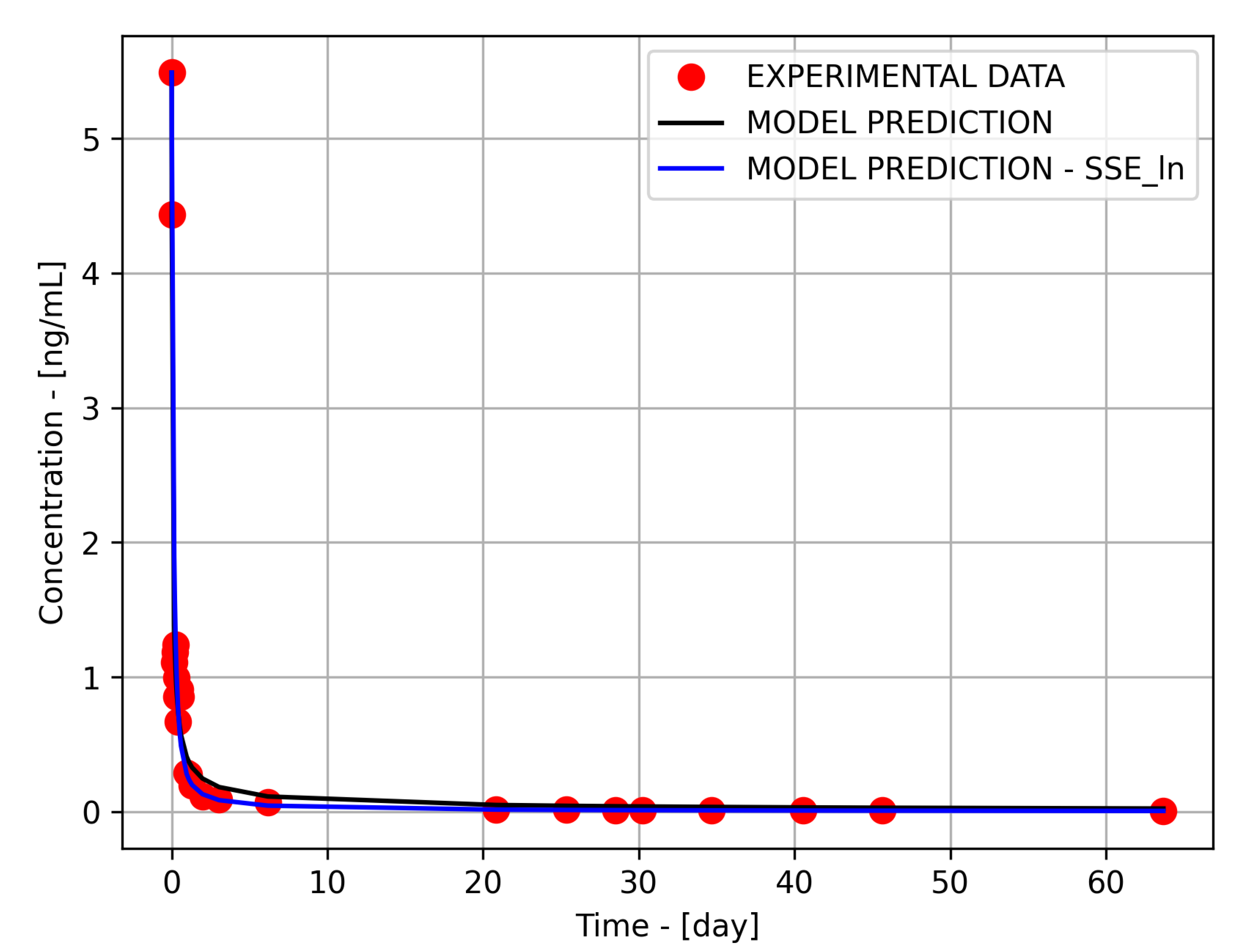
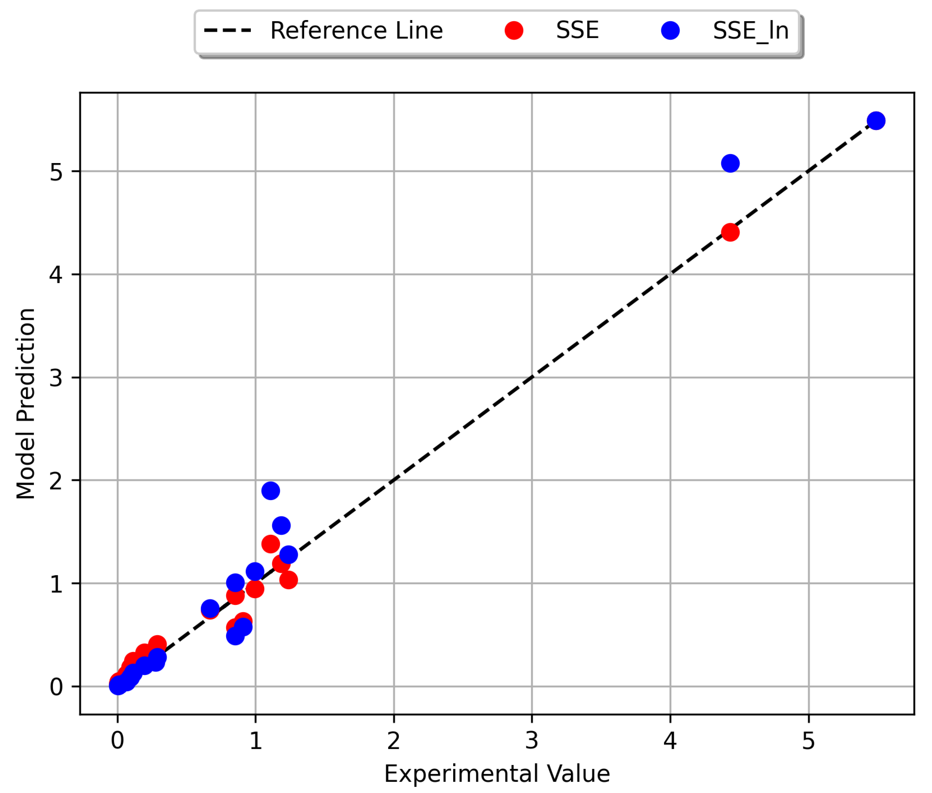
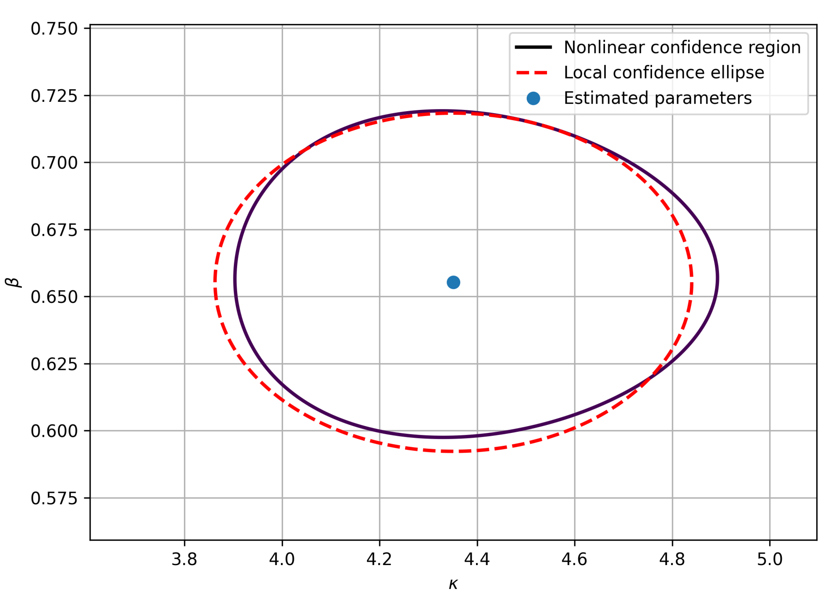
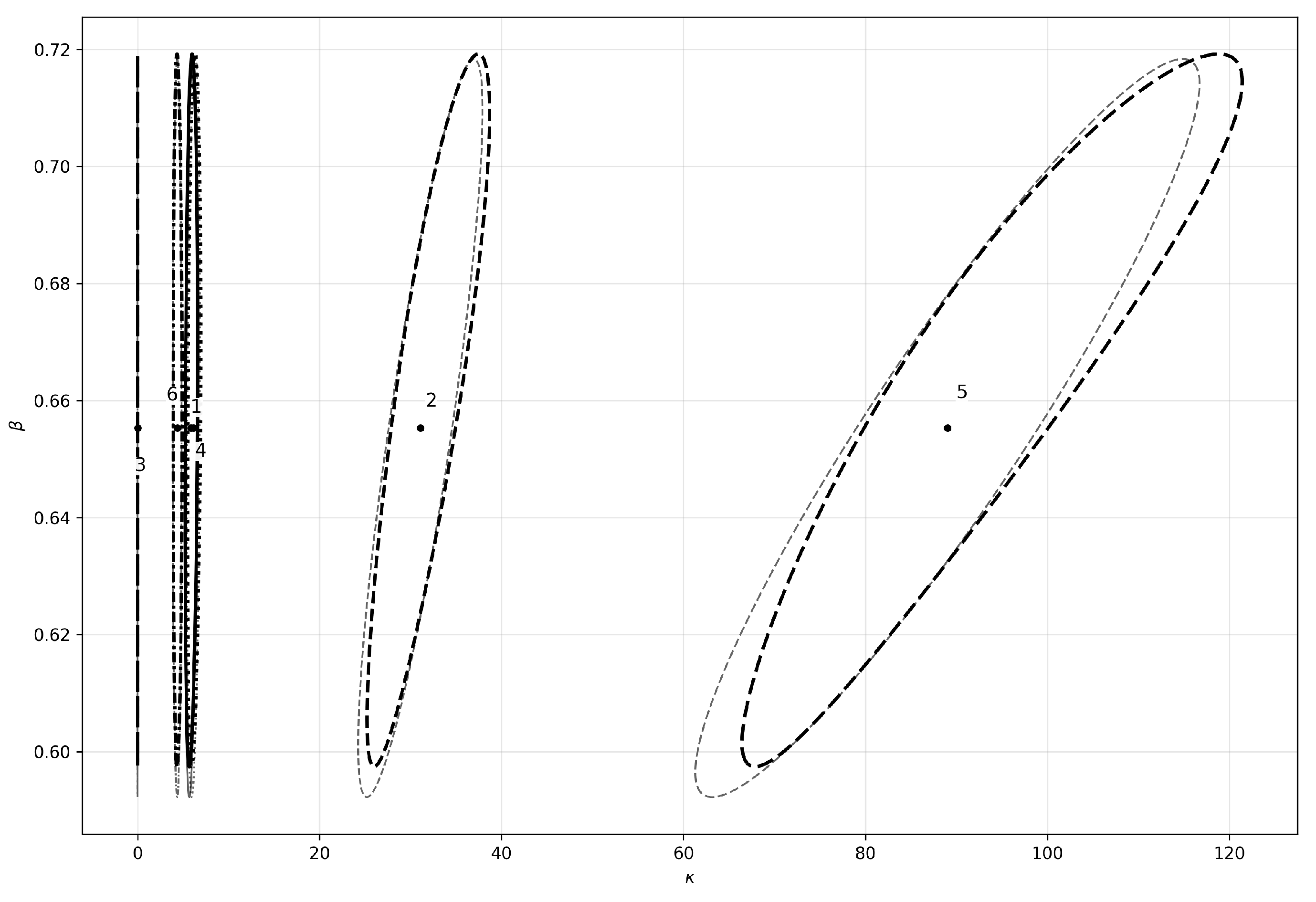
Figure 1 and Figure 2 present the model prediction and dynamic behavior of the experimental data and the model prediction versus the experimental data plot, considering SSE given by Equation (7) and $SS{E}_{ln}=\sum {(ln{\left(C_i\right)}_{exp}-ln{\left(C_i\right)}_{model})}^2$. It can be seen that the model presented good agreement considering the new estimation procedure, and therefore, the choice of scale of the dependent variable did not influence the quality of the fit. The linear confidence ellipses (Equation (14)) and the nonlinear confidence regions (Equation (15)) are shown in Figure 3 for the parameters estimated considering the methodology proposed in this work. The local ellipse became nearly aligned with the coordinate axes because the covariance term was approximately zero. The nonlinear region was not forced to be exactly elliptical, but its orientation was consistent with the local covariance structure. Thus, the covariance vanishing scale improved the interpretability of the estimates, as the uncertainty in $\kappa$ can be discussed with minimal first-order interference approximation from uncertainty in $\beta$, and vice versa. Finally, Figure 4 presents the confidence regions for all cases, particularly (1)$t_{ref}=1.0$; (2) $t_{ref}=13.34$ (arithmetic mean); (3) $t_{ref}=0.1175$ (harmonic mean); (4) $t_{ref}=2.175$ (geometric mean); (5) $t_{ref}=63.69$ (maximum t value); and (6) $t_{ref}=0.6365$ (vanishing covariance). It can be observed that the sign of the parameter correlation resulted in a right (regions 1, 2, 4, and 5) or left inclination (region 3) of the region, while region 6 had rough to no inclination due to the parameter correlation value.

Figure 5 presents the histogram of the residuals, defined as ${\left(C_i\right)}_{exp}-{\left(C_i\right)}_{model}$, and Figure 6 presents the corresponding normal Q–Q plot. The residuals were centered close to zero, with a mean equal to $-0.0151$ and standard deviation equal to $0.1211$, indicating the absence of a strong systematic bias in the fitted concentration scale. However, the Q–Q plot shows deviations in the tails, suggesting that the residual distribution should not be interpreted as strictly Gaussian. Therefore, the confidence regions reported in this work should be understood approximate local inferential tools based on the least-squares and Gauss–Newton framework. This limitation does not affect the main conclusion of this study because the comparison among reference-time strategies was based on the same objective function, the same residual vector, and the same fitted trajectory.

For model identification, these results indicate that the reference-time scaling procedure should be an interesting alternative tool for parameter estimation, but it is important to stress that it does not modify the physical model or change the curve behavior that would be obtained with the original parameters. The arithmetic, harmonic, and geometric means are useful descriptive scales, but they are not guaranteed to minimize the covariance. The optimal reference time obtained by the methodology proposed in this work is model- and data-dependent, because it was determined from the sensitivity matrix evaluated at the least-squares solution. Consequently, $t_{ref}$ should be interpreted as the reference time that best conditions the local estimation problem for the available experimental design.

3.2. Case Study-02

In Case Study-02, the mathematical analysis considered experimental data of open-loop tests performed on a didactic thermal process control system. The study considered the fractional model (Equation (54)). The expression of $f\left(t\right)$ was considered a Heaviside function with a magnitude obtained from the voltage step and the gain of the process. Test 02 was performed to validate the system gain to be $0.57$ °C/${\mathrm{V}}_{AC}$, and Test 01 data were used for parameter estimation. Therefore, $f\left(t\right)=(T(t=0)$ °C $+(0.57$ °C/${\mathrm{V}}_{AC}·44.1$ ${\mathrm{V}}_{AC}\left)\right)·Heaviside\left(t\right)$, where $T(t=0)=26.9$ °C in Test 01.

Since the steady-state gain used in the forced model was obtained from an independent experiment, an additional sensitivity analysis was performed to evaluate whether small variations in the gain affected the proposed reference-time scaling. The estimation procedure was repeated using the gains obtained from Test 01 and Test 02, as well as the rounded value $0.57$ °C $/V_{AC}$ used in the main analysis. The estimated values of m and $\beta$ changed only slightly, whereas the qualitative covariance behavior remained unchanged. Conventional choices of $t_{ref}$ produced non-zero parameter correlations, while the sensitivity-based reference time reduced the local correlation between $\mu$ and $\beta$ to zero. Therefore, the main conclusion of the thermal case study is robust with respect to the small experimental variation observed in the independently determined process gain.

Table 4. Summary of the estimation results for different $t_{ref}$ values: Case Study-02.

Reference-Time Strategy	${\mathit{t}}_{\mathit{ref}}$$\left[\mathit{h}\right]$	$\mathit{\mu }$	$\mathit{\rho }(\mathit{\mu },\mathit{\beta })$	${\mathit{V}}_{\mathit{\theta }}$ Equation (79)
None	1.0	$0.2413\pm 0.00527$	−0.366	$\left[\begin{array}{cc}3.084·{10}^{-5}& -3.132·{10}^{-5}\\ -3.132·{10}^{-5}& 2.369·{10}^{-4}\end{array}\right]$
Maximum t value	0.9210	$0.2620\pm 0.005865$	−0.317	$\left[\begin{array}{cc}3.474·{10}^{-5}& -2.881·{10}^{-5}\\ -2.881·{10}^{-5}& 2.369·{10}^{-4}\end{array}\right]$
Arithmetic mean	0.4605	$0.5055\pm 0.01092$	0.161	$\left[\begin{array}{cc}1.204·{10}^{-4}& 2.699·{10}^{-5}\\ 2.699·{10}^{-5}& 2.369·{10}^{-4}\end{array}\right]$
Harmonic mean	0.000200	$815.6\pm 101.0$	0.985	$\left[\begin{array}{cc}1.042·{10}^{+4}& 1.5474\\ 1.5474& 2.369·{10}^{-4}\end{array}\right]$
Geometric mean	0.2174	$1.034\pm 0.02694$	0.574	$\left[\begin{array}{cc}7.331·{10}^{-4}& 2.389·{10}^{-4}\\ 2.389·{10}^{-4}& 2.369·{10}^{-4}\end{array}\right]$
This work	0.5780	$0.4070\pm 0.008676$	$3.69·{10}^{-10}$	$\left[\begin{array}{cc}7.624·{10}^{-5}& 4.959·{10}^{-14}\\ 4.959·{10}^{-14}& 2.369·{10}^{-4}\end{array}\right]$

presents the estimation results, using temperature values as the dependent variable and time as the independent variable. Similar to the previous study, the experimental data were fitted considering five different approaches for $t_{ref}$, and $t_{ref}=1.0$ was also considered. As expected, the fitted temperature profile was invariant with respect to the reference-time strategy. The residual sum of squares remained constant for all choices of $t_{ref}$, with $SSE\approx 4.73$. Also, $\beta =0.9540\pm 0.01530$ was obtained for all approaches. The recovered dimensional coefficient was $m=0.2413$ h^β, while the scaled coefficient $\mu =m/t_{ref}^{\beta }$ varied according to the selected reference time. For example, for the covariance-vanishing reference time, $t_{ref}=0.5780$ h, the estimated scaled coefficient was $\mu =0.4070$, which corresponds to $m=0.2413$ h^β.

In this case study, parameter correlations were either positive or negative according to the value of $t_{ref}$. The proposed methodology reduced the correlation to $\rho =3.69·{10}^{-10}$, roughly eliminating the local covariance between $\mu$ and $\beta$ at the numerical precision of the calculation. As in the kinetics case study of this work, the results obtained here also show that the covariance reduction was not produced by a different fit, because the residual surface minimum continued unchanged. Instead, it resulted from a change in coordinates that made the sensitivity column associated with $\beta$ locally orthogonal to the sensitivity column associated with $\mu$.

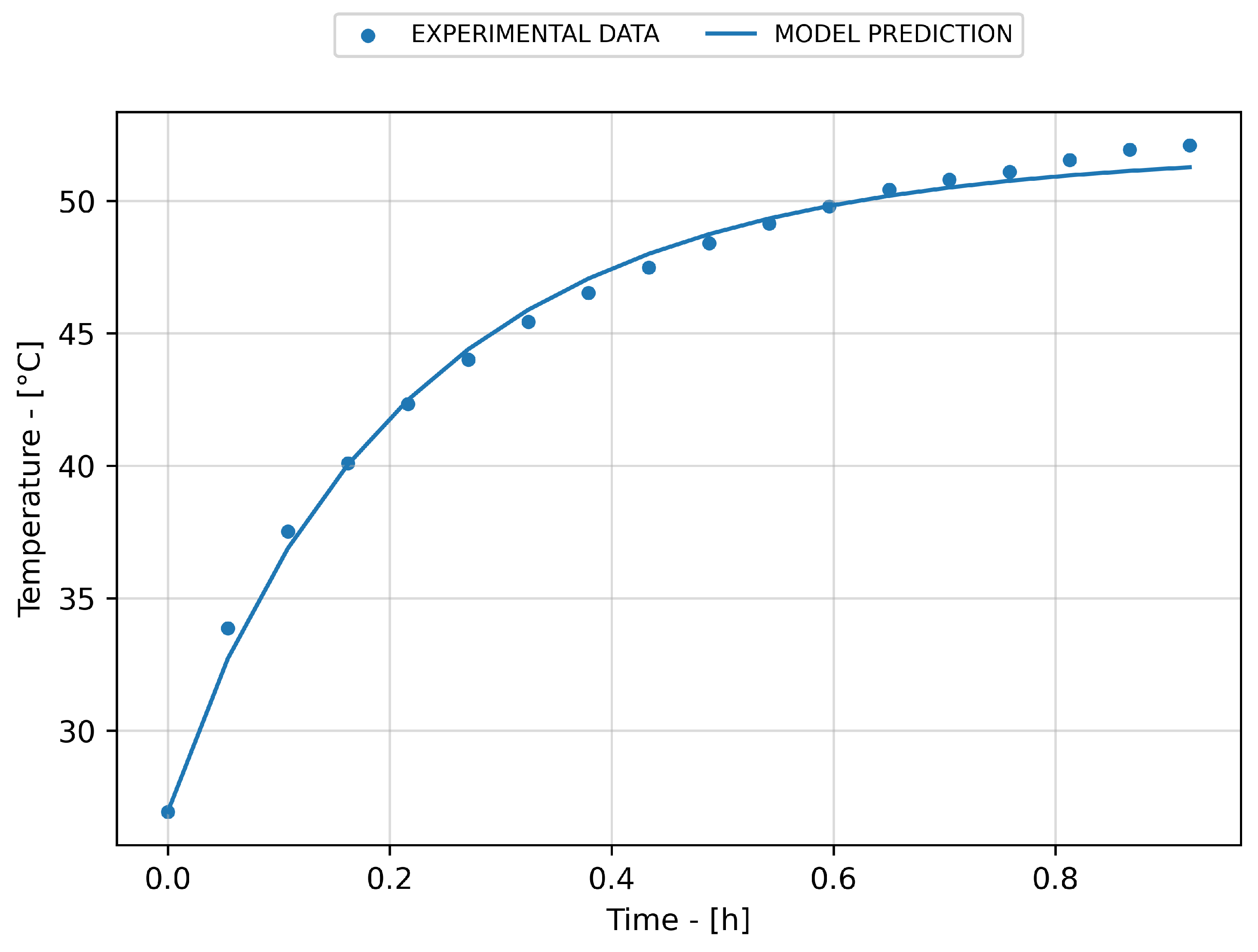
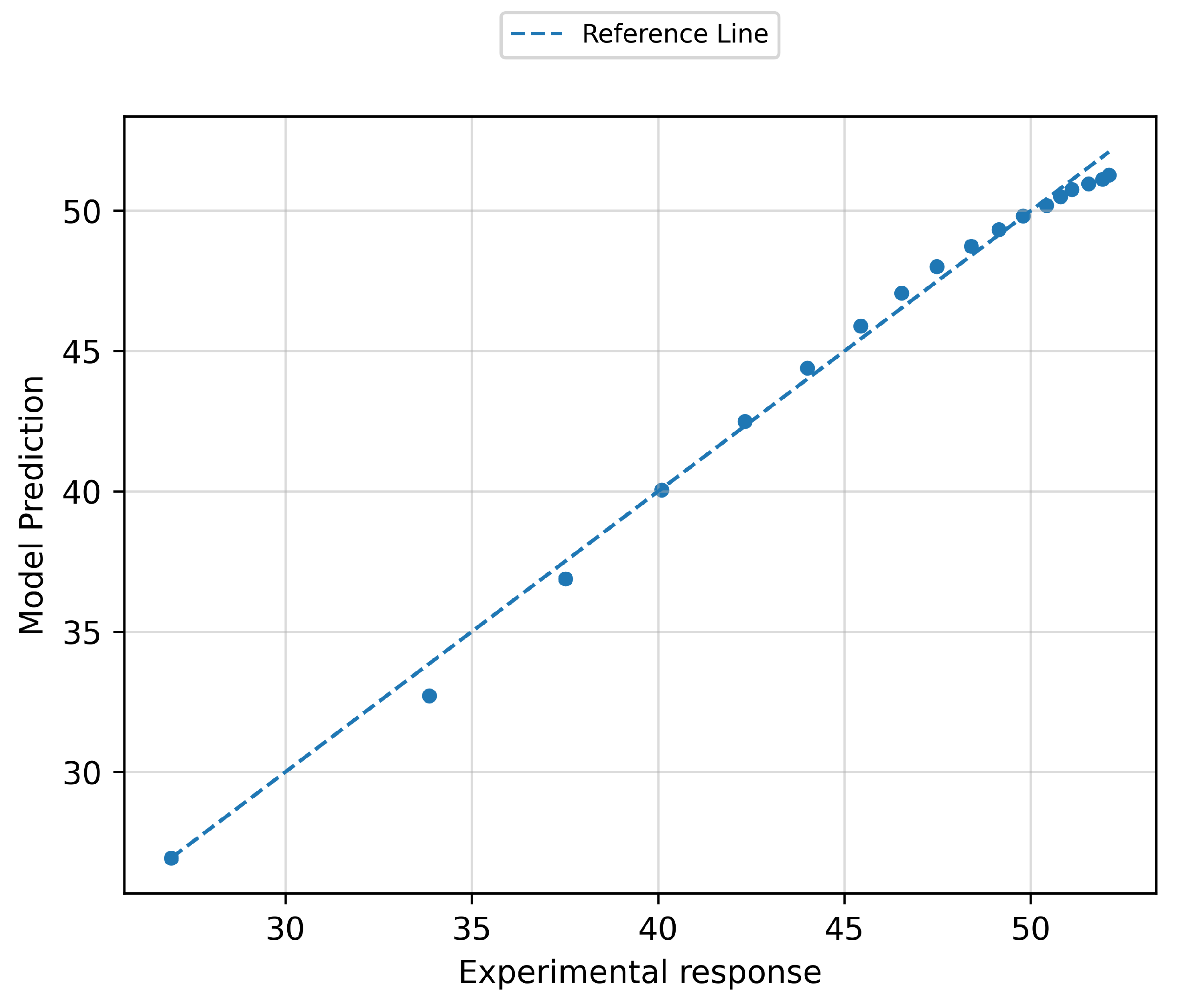
Figure 7 and Figure 8 present the model prediction and experimental data dynamic behavior and the model prediction versus experimental data plots. It can be seen that the model predictions agreed with the experimental data when considering the new estimation procedure.

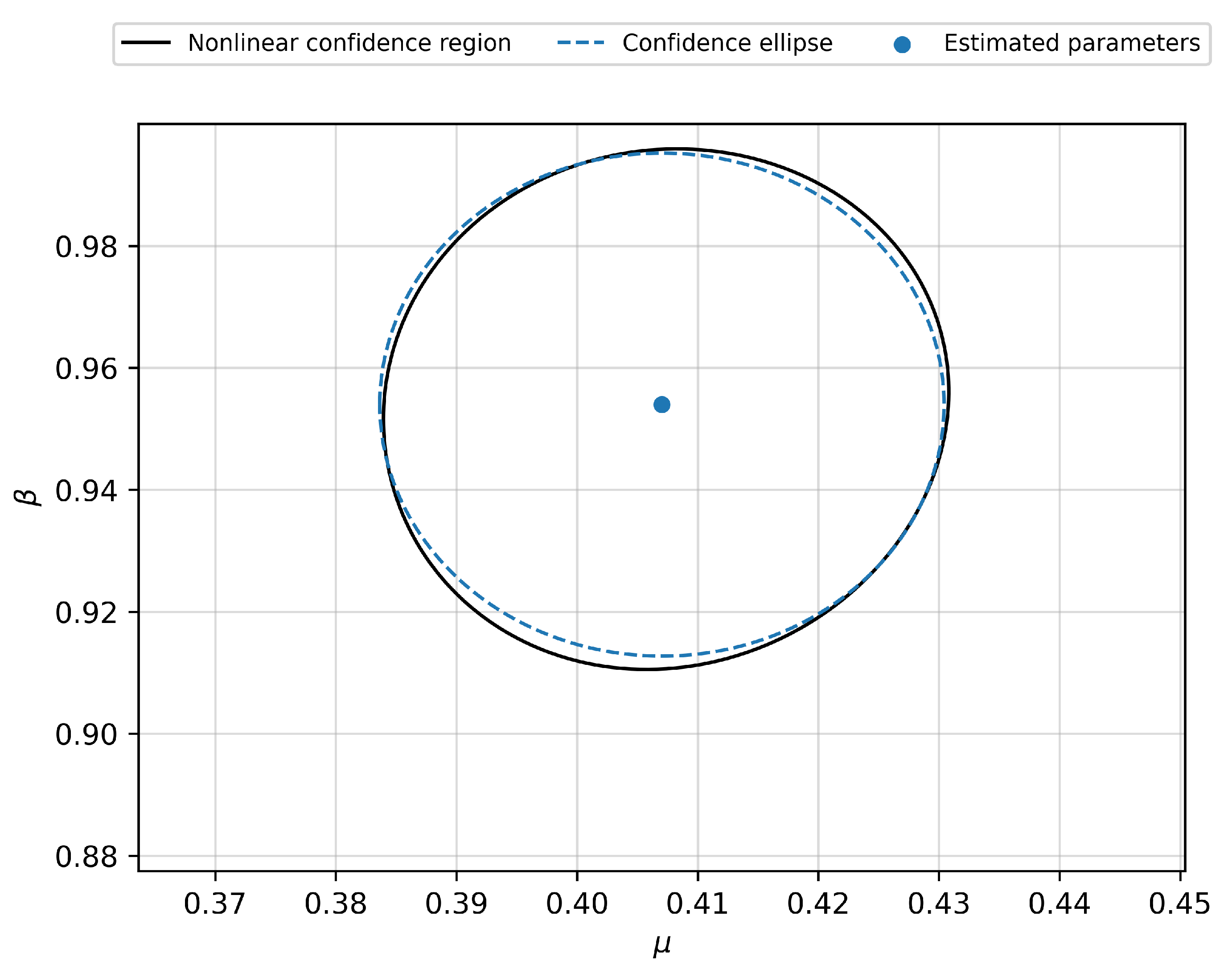
The linear confidence ellipses (Equation (14)) and the nonlinear confidence regions (Equation (15)) are shown in Figure 9 for the parameters estimated when considering the methodology proposed in this work. The local ellipse became nearly aligned with the coordinate axes, because the covariance term was approximately zero. The nonlinear region was not forced to be exactly elliptical, but its orientation was consistent with the local covariance structure. Thus, the covariance-vanishing scale improved the interpretability of the estimates, as the uncertainty in $\mu$ could be discussed with minimal interference from uncertainty in $\beta$, and vice versa. For all reference-time choices, the fitted trajectory, residual sum of squares, fractional order, and recovered dimensional coefficient remained invariant, whereas the proposed covariance-vanishing reference time reduced the local correlation between $\mu$ and $\beta$ to zero.

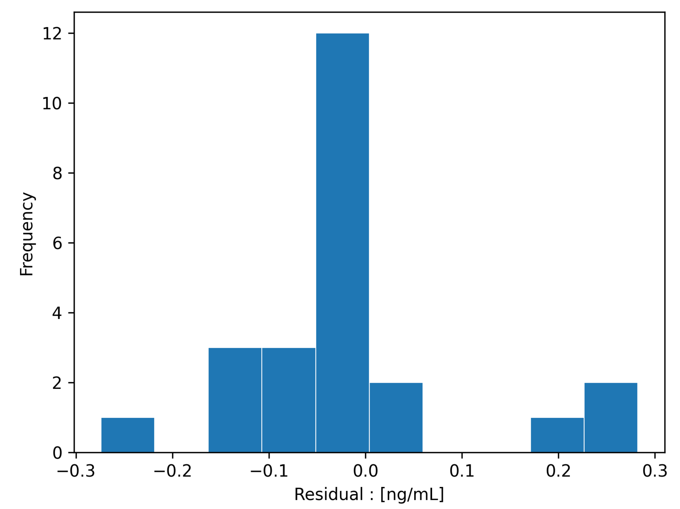
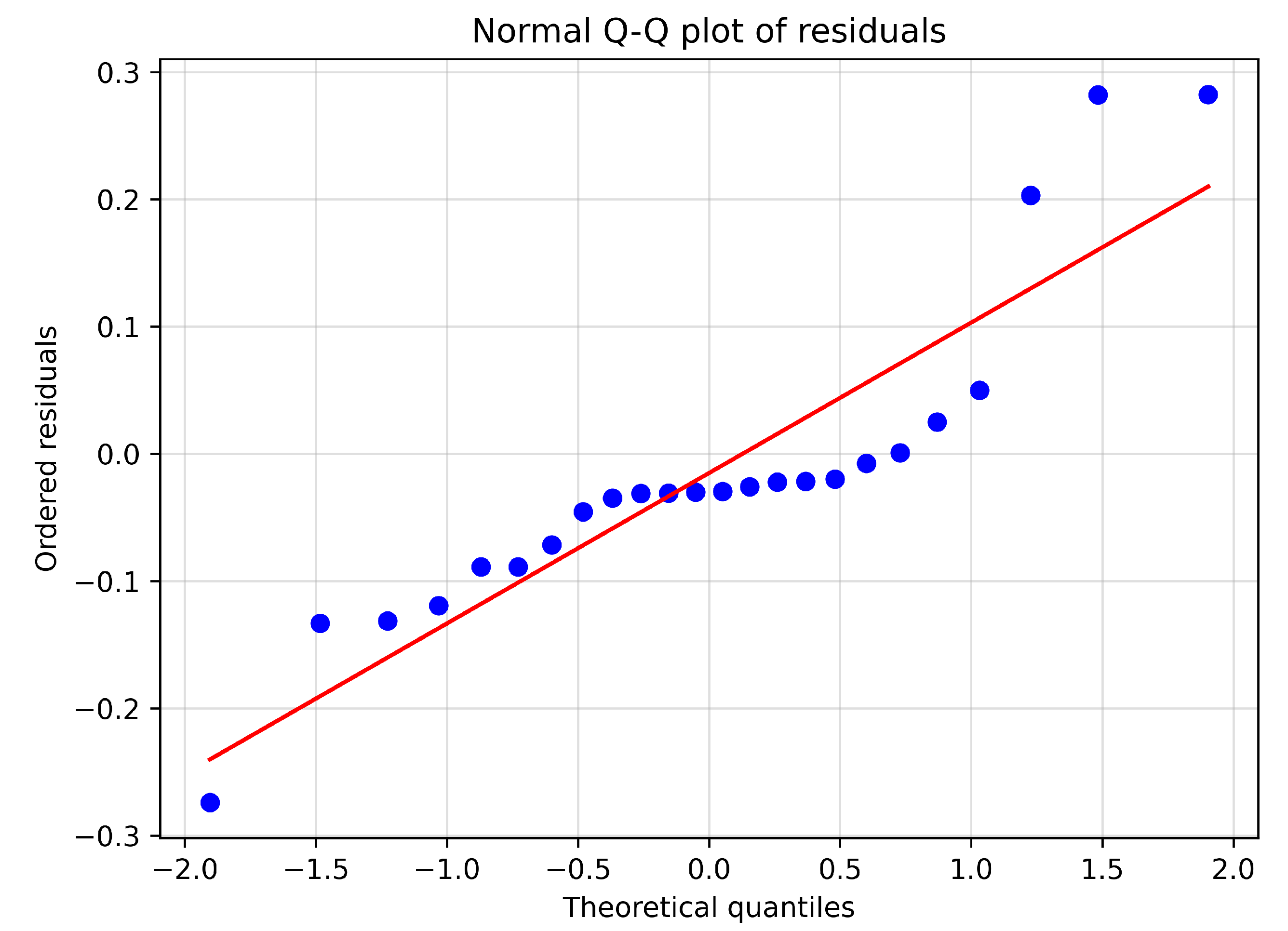
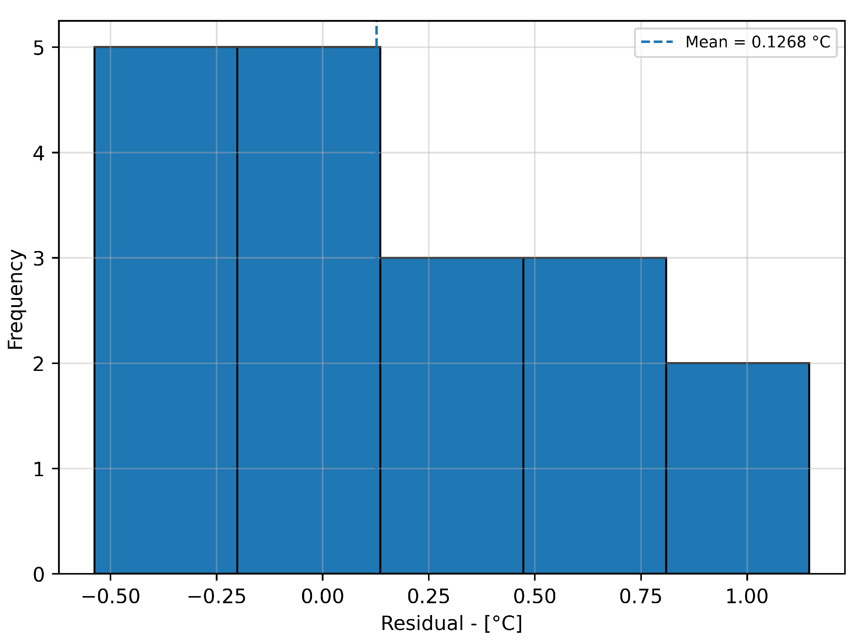
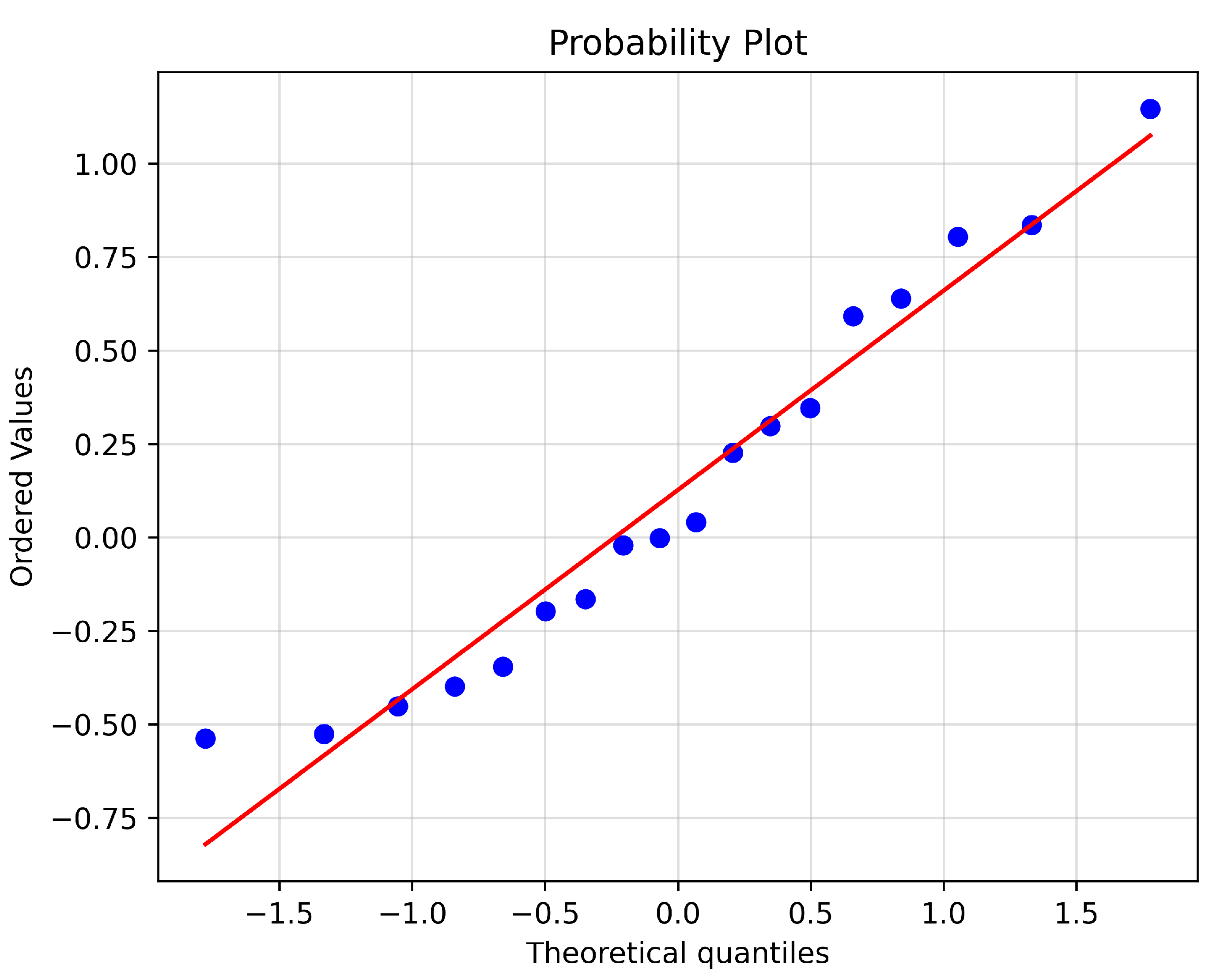
Figure 10 presents the histogram of the residuals, and Figure 11 presents the normal Q–Q plot. The residuals were concentrated mainly in the interval $(-0.5,0.5)$ °C, with a mean equal to $0.127$ °C and standard deviation equal to $0.516$ °C. The Shapiro–Wilk test did not reject the normality hypothesis for this dataset. Nevertheless, because the sample size was limited, and some residual structure was still visible over time, the residual analysis should be interpreted as compatible with approximate normality rather than as definitive evidence of Gaussian errors. The main purpose of this case study is therefore not to prove a complete stochastic error model but to demonstrate that reference-time scaling changes the local covariance structure while preserving the fitted model response.

3.3. Practical Implications and Scope of the Reference-Time Scaling

The proposed reference-time scaling is most relevant when the dimensionless kinetic coefficient and the fractional order are estimated simultaneously and exhibit strong local correlation. In these problems, changes in one parameter may be locally compensated by changes in the other, leading to inclined or elongated confidence regions and making their individual effects and uncertainties difficult to interpret. In the present case studies, conventional reference-time choices produced absolute local correlations as high as 0.9327 for the fractional decay model and 0.985 for the forced fractional model. In contrast, the sensitivity-based reference time reduced the corresponding correlations to $5.566·{10}^{-9}$ and $3.69·{10}^{-10}$. This reduction leaves the local confidence regions closer to the parameter axes and permits the marginal uncertainties of the dimensionless coefficient and $\beta$ to be interpreted with minimal first-order mutual interference.

This feature may be particularly useful when the physical interpretation of the fractional order is central to the analysis, when parameter estimates must be compared across experiments or operating conditions, or when strong parameter compensation produces poorly scaled estimation problems. The transformation also provides a systematic alternative to selecting the reference time from descriptive measures of the experimental times, such as their arithmetic, geometric, or harmonic means. Because the proposed reference time is derived from the fitted sensitivity structure, it is specific to the model, parameter estimates, and experimental design.

However, the proposed procedure is a reparameterization of the same physical model. Therefore, it does not improve the fitted trajectory, residual sum of squares, point predictions, fractional order estimate, or recovered dimensional coefficient. Its primary demonstrated benefit is the improvement of local inferential interpretability under the Gauss–Newton approximation. When incorporated into the iterative estimation procedure, the improved local conditioning may also contribute to numerical robustness in highly correlated or poorly scaled problems. Nevertheless, possible improvements in convergence speed, robustness to initial guesses, and reductions in optimization failure rates were not quantitatively evaluated and therefore remain to be demonstrated. Finally, it is worth mentioning that the applicability demonstrated here is restricted to the two linear first-order fractional formulations investigated, and the present results should not be extrapolated directly to nonlinear, multiparameter, distributed-order, or variable-order fractional models.

4. Conclusions

This work proposed a sensitivity-based reference-time scaling strategy for local reparameterization of two linear fractional-order models. The method was developed for a fractional decay model and a forced fractional step response model. In both cases, the dimensional model parameter and the fractional order were structurally coupled through the non-integer power of time and the Mittag-Leffler response. This coupling may appear as local covariance between the estimated model coefficient and the fractional order.

The proposed reference time was derived from the local sensitivity matrix by imposing a zero off-diagonal term in the Gauss–Newton information matrix. As a result, the dimensionless coefficient and the fractional order become locally orthogonal under the first-order approximation. The transformation does not modify the governing model, the fitted trajectory, the residual sum of squares, the fractional order, or the recovered dimensional coefficient. It only changes the coordinate system in which the uncertainty of the estimated parameters is represented.

In the two case studies analyzed, conventional reference-time choices, such as the maximum experimental time and arithmetic, geometric, or harmonic means of the sampling times, did not consistently reduce the local correlation between the dimensionless parameter and $\beta$. In contrast, the sensitivity-based reference time reduced the corresponding Gauss–Newton local correlation to zero for the fitted models, as expected from its construction. These results suggest that the proposed scaling can be useful as a post-estimation reparameterization tool for improving the first-order statistical interpretation of the two fractional-order formulations considered here.

Therefore, the method should not be interpreted as a global solution to parameter identifiability, nonlinear parameter dependence, or multiparameter decorrelation. Its validity is local and depends on the Gauss–Newton approximation, the residual structure, the numerical accuracy of the sensitivity matrix, and the information content of the experimental data. The present validation is restricted to the two linear first-order fractional formulations considered in this work. Extension to nonlinear, multiparameter, distributed-order, and variable-order fractional models, together with higher-order uncertainty analyses, should therefore be investigated in future work to assess the broader applicability of the proposed approach.

References

1. Zaslavsky, G.M. Chaos, fractional kinetics, and anomalous transport. Phys. Rep. 2002, 371, 461–580. [Google Scholar] [CrossRef] [Scilit]
2. Cherifi, L.; Ammi, Y.; Hanini, S.; Bailek, N.; El-Kenawy, E.-S.M.; Younis, J.A.; Zerouali, B.; Dahmani, A.; Colak, I.; Almaliki, A.H. A generalized fractional model for one-step identification of membrane filtration clogging mechanisms. Sci. Rep. 2026, 16, 3649. [Google Scholar] [CrossRef] [Scilit] [PubMed]
3. Li, M.; He, J. Fractional processes and systems in computer science and engineering. Fractal Fract. 2026, 10, 198. [Google Scholar] [CrossRef] [Scilit]
4. Dokoumetzidis, A.; Macheras, P. Fractional kinetics in drug absorption and disposition processes. J. Pharmacokinet. Pharmacodyn. 2009, 36, 165–178. [Google Scholar] [CrossRef] [Scilit] [PubMed]
5. Khan, Z.A.; Khan, T.A.; Waqar, M.; Chaudhary, N.I.; Raja, M.A.Z.; Shu, C.M. Nonlinear marine predator algorithm for robust identification of fractional hammerstein nonlinear model under impulsive noise with application to heat exchanger system. Commun. Nonlinear Sci. Numer. Simul. 2025, 146, 108809. [Google Scholar] [CrossRef] [Scilit]
6. Schwaab, M.; Pinto, J.C. Optimum reference temperature for reparameterization of the Arrhenius equation. Part 1: Problems involving one kinetic constant. Chem. Eng. Sci. 2007, 62, 2750–2764. [Google Scholar] [CrossRef] [Scilit]
7. Box, G.E.P.; Cox, D.R. An analysis of transformations. J. R. Stat. Soc. Ser. B (Methodol.) 1964, 26, 211–243. [Google Scholar] [CrossRef] [Scilit]
8. Cox, D.; Reid, N. Parameter orthogonality and approximate conditional inference. J. R. Stat. Soc. Ser. B (Methodol.) 1987, 49, 1–18. [Google Scholar] [CrossRef] [Scilit]
9. Friesen, V.C.; Leitoles, D.P.; Gonçalves, G.; Lenzi, E.K.; Lenzi, M.K. Modeling heavy metal sorption kinetics using fractional calculus. Math. Probl. Eng. 2015, 2015, 549562. [Google Scholar] [CrossRef] [Scilit]
10. Guo, Y.; Ma, B.; Wu, R. On sensitivity analysis of parameters for fractional differential equations with Caputo derivatives. Electron. J. Qual. Theory Differ. Equ. 2016, 2016, 1–17. [Google Scholar] [CrossRef] [Scilit]
11. Victor, S.; Malti, R.; Garnier, H.; Oustaloup, A. Parameter and differentiation order estimation in fractional models. Automatica 2013, 49, 926–935. [Google Scholar] [CrossRef] [Scilit]
12. Caputo, M. Linear models of dissipation whose Q is almost frequency independent—II. Geophys. J. Int. 1967, 13, 529–539. [Google Scholar] [CrossRef] [Scilit]
13. Diethelm, K. The Analysis of Fractional Differential Equations: An Application-Oriented Exposition Using Differential Operators of Caputo Type; Lecture Notes in Mathematics; Springer: Berlin/Heidelberg, Germany, 2010; Volume 2004. [Google Scholar] [CrossRef] [Scilit]
14. Podlubny, I. Fractional Differential Equations: An Introduction to Fractional Derivatives, Fractional Differential Equations, to Methods of Their Solution and Some of Their Applications; Mathematics in Science and Engineering; Academic Press: San Diego, CA, USA, 1999; Volume 198. [Google Scholar] [CrossRef] [Scilit]
15. de Oliveira, E.C.; Jarosz, S.; Vaz, J., Jr. Fractional calculus via Laplace transform and its application in relaxation processes. Commun. Nonlinear Sci. Numer. Simul. 2018, 69, 58–72. [Google Scholar] [CrossRef] [Scilit]
16. Euler, L. De progressionibus transcendentibus seu quarum termini generales algebraice dari nequeunt. Comment. Acad. Sci. Petropolitanae 1738, 5, 36–57. [Google Scholar]
17. Bard, Y. Nonlinear Parameter Estimation, 1st ed.; Academic Press: New York, NY, USA, 1974. [Google Scholar]
18. Pavlenko, I.; Ochowiak, M.; Włodarczak, S.; Krupińska, A.; Matuszak, M. Parameter Identification of the Fractional-Order Mathematical Model for Convective Mass Transfer in a Porous Medium. Membranes 2023, 13, 819. [Google Scholar] [CrossRef] [Scilit] [PubMed]
19. Ji, C.C.; Dai, W.; Mickens, R.E. A fractional-order alternative for phase-lagging equation. Int. J. Numer. Anal. Model. 2023, 20, 391–406. [Google Scholar] [CrossRef] [Scilit]
20. Mainardi, F.; Gorenflo, R. Time-fractional derivatives in relaxation processes: A tutorial survey. Fract. Calulus Appl. Anal. 2007, 10, 269–308. [Google Scholar] [CrossRef] [Scilit]
21. Flores-Tlacuahuac, A.; Biegler, L.T. Optimization of fractional order dynamic chemical processing systems. Ind. Eng. Chem. Res. 2014, 53, 5110–5127. [Google Scholar] [CrossRef] [Scilit]
22. Himmelblau, D. Process Analysis by Statistical Methods, 1st ed.; John Wiley & Sons: New York, NY, USA, 1970. [Google Scholar]
23. Mittag-Leffler, M. Sur la nouvelle fonction. Comptes Rendus Acad. Sci. 1903, 137, 554–558. [Google Scholar]
24. Weiss, M. The anomalous pharmacokinetics of amiodarone explained by nonexponential tissue trapping. J. Pharmacokinet. Biopharm. 1999, 27, 383–396. [Google Scholar] [CrossRef] [Scilit] [PubMed]
25. Cripa, C. Aplicação de Controle Fuzzy a Sistemas Térmicos. Master’s Thesis, Universidade Federal do Paraná, Curitiba, Brazil, 2020. (In Portuguese) [Google Scholar]
26. Garrappa, R. Numerical evaluation of two and three parameter Mittag-Leffler functions. SIAM J. Numer. Anal. 2015, 53, 1350–1369. [Google Scholar] [CrossRef] [Scilit]
27. Python Core Team. Python: A Dynamic, Open Source Programming Language, version 3.12; Python Software Foundation (PSF): Beaverton, OR, USA, 2024.
28. Harris, C.R.; Millman, K.J.; van der Walt, S.J.; Gommers, R.; Virtanen, P.; Cournapeau, D.; Wieser, E.; Taylor, J.; Berg, S.; Smith, N.J.; et al. Array programming with NumPy. Nature 2020, 585, 357–362. [Google Scholar] [CrossRef] [Scilit] [PubMed]
29. Virtanen, P.; Gommers, R.; Oliphant, T.E.; Haberland, M.; Reddy, T.; Cournapeau, D.; Burovski, E.; Peterson, P.; Weckesser, W.; Bright, J.; et al. SciPy 1.0: Fundamental Algorithms for Scientific Computing in Python. Nat. Methods 2020, 17, 261–272. [Google Scholar] [CrossRef] [Scilit] [PubMed]
30. Biolek, D.; Garrappa, R.; Mainardi, F.; Popolizio, M. Derivatives of Mittag-Leffler functions: Theory, computation and applications. Nonlinear Dyn. 2025, 113, 34389–34403. [Google Scholar] [CrossRef] [Scilit]
Figure 1. Model prediction and experimental data dynamic behavior: Case Study 01.
Processes 14 02588 g001
Figure 2. Model prediction versus experimental data: Case Study 01.
Processes 14 02588 g002
Figure 3. Local parameter confidence Region (Gauss–Newton Approximation), κ = 4.351 and β = 0.6553 : Case Study-01.
Processes 14 02588 g003
Figure 4. Effect of reference-time scaling on confidence regions for all cases: Case Study-01 (dashed gray region: Equation (14)/dashed black region: Equation (15)).
Processes 14 02588 g004
Figure 5. Histogram of residuals: Case Study-01.
Processes 14 02588 g005
Figure 6. Normal Q–Q plot of residuals: Case Study-01.
Processes 14 02588 g006
Figure 7. Model prediction and experimental data dynamic behavior: Case Study 02.
Processes 14 02588 g007
Figure 8. Model prediction versus experimental data: Case Study 02.
Processes 14 02588 g008
Figure 9. Parameter confidence region (Gauss–Newton approximation), μ = 0.4070 and β = 0.9540 : Case Study-02.
Processes 14 02588 g009
Figure 10. Histogram of residuals: Case Study-02.
Processes 14 02588 g010
Figure 11. Normal Q–Q plot of residuals: Case Study-02.
Processes 14 02588 g011