Article

A Dual-Track Feature-Enhanced Physics-Informed Model for Accurate Wind Power Forecasting with Physical Consistency

1
College of Information, Shanghai Ocean University, Shanghai 201306, China
2
School of Electromechanical and Automotive Engineering, Yantai University, Yantai 264005, China
*
Authors to whom correspondence should be addressed.
Processes 2026, 14(16), 2560; https://doi.org/10.3390/pr14162560
Submission received: 7 July 2026 / Revised: 24 July 2026 / Accepted: 3 August 2026 / Published: 11 August 2026

Abstract

In response to stochastic fluctuations in large-scale wind power integration and the resulting peak-shaving challenges, high-precision forecasting with physical consistency is essential for grid safety. To address the inefficiency of physical models and poor interpretability of data-driven methods, this paper proposes a hybrid FCM-WGM-BiLSTM-Transformer (FW-BTP) framework integrating Fuzzy C-Means (FCM) clustering, Weighted Grey Model (WGM) trend extraction, and a coupled BiLSTM-Transformer module. Physical prior knowledge—wind turbine power curves—is embedded into the loss function via a Physics-Guided Loss Regularization (PGL) mechanism. Validated on measured data from a Xinjiang wind farm, the model achieves an R 2 of 0.9967, MAE of 6.11, and RMSE of 11.19. The proposed model reduces R 2 by 37% compared to the newer model KAN, and compared to the better-performing recurrent baseline model (BiLSTM, MAE = 8.75 MW), the proposed FW-BTP model reduces the MAE by 30% (to 6.12 MW). Ablation studies confirm the WGM reduces LogCosh loss from 9.57 to 5.12, and SHAP analysis verifies sensitivity to trend and physical wind speed features. The framework balances accuracy, robustness, and interpretability, supporting refined scheduling in modern power systems.

1. Introduction

As the global energy transition continues to advance, wind power—the most mature form of renewable energy for large-scale development—poses significant challenges to the real-time balance and safety control of power system operations due to its large-scale grid integration. The intermittent and fluctuating nature of wind power output is primarily governed by meteorological factors, making high-precision power forecasting a key technology for ensuring grid absorption capacity and optimizing dispatch decisions. With advancements in the Internet of Things (IoT) and numerical weather prediction technologies, data-driven methods have become dominant in the forecasting field; however, accurately identifying and learning complex and variable weather-output mapping patterns from historical data remains the core bottleneck in improving model performance.
Wind power forecasting refers to the estimation of a power plant’s output power for a specific future time period by integrating historical power data, meteorological forecast information, and temporal characteristics. Forecasting accuracy directly impacts the economic efficiency and reliability of the power system: in day-ahead markets, forecast results support the formulation of generation schedules and trading bids; in real-time dispatch, ultra-short-term forecasts are used to rapidly adjust reserve capacity in response to disturbances such as extreme wind speed fluctuations; for microgrids with a high proportion of wind power integration, accurate forecasting is a prerequisite for achieving coordinated control of generation, load, and storage, and maintaining stable system operation. Therefore, developing intelligent forecasting models capable of adapting to different weather types and possessing strong generalization capabilities holds significant practical importance for advancing the construction of new power systems.
Existing wind power forecasting methods can be categorized into physics-driven models and data-driven models based on their technical architecture [1]. Physics-driven models, typified by energy system planning tools, construct optimization models based on the economic parameters and physical constraints of energy technologies [2]. They use methods such as linear programming to determine the lowest-cost energy system configuration and can perform structured, multi-sector coordinated simulations of long-term energy transition scenarios. Employing flexible time-slice techniques to decompose intraday and seasonal electricity demand curves, it can more accurately characterize the role of energy storage technologies in the power system, providing quantitative support for optimizing energy storage deployment on both the supply and demand sides. Furthermore, the wind farm physical modeling chain [3] represents another significant branch. By modeling physical mechanisms such as wind turbine power characteristic curves and the impact of terrain on wind speed evolution [4], it enables the optimization of capacity allocation for distributed wind power and energy storage devices under power balance constraints. The advantage of such models lies in their rigorous logic and solid theoretical foundation, which fully reflect the physical nature of energy systems. However, their limitations are equally evident: complex model structures result in high computational costs and stringent hardware requirements; simultaneously, they exhibit a delayed response to sudden meteorological fluctuations, failing to capture short-term system changes in a timely manner [5]. Some physical models rely on high-precision input data (such as mesoscale numerical weather prediction data), and errors in the raw data are directly propagated to the prediction results, requiring additional error correction [6].
Data-driven models do not require predefined physical mechanisms but instead directly mine the relationships between variables from historical data. Based on their technical approaches, they can be categorized into traditional statistical models and machine learning models, with the latter further subdivided into deterministic and non-deterministic forecasting subtypes. Traditional statistical models primarily include time-series analysis and regression methods. In addition to the classic ARIMA model, autoregressive moving average (ARMA) models are suitable for forecasting stationary energy time-series data. The seasonal autoregressive integrated moving average (SAARMA) model [7] introduces a seasonal difference term, specifically targeting data with pronounced seasonal fluctuations, such as wind power generation. Vector autoregressive (VAR) models [8] overcome the limitations of univariate analysis and support forecasting under the influence of multiple factors. Among regression methods, geographically weighted regression [9] captures the differentiated impact of regional topography on wind energy development by introducing spatial weighting coefficients. The core limitations of such models lie in their inability to describe the complex nonlinear interactions between wind power output and multiple factors such as meteorological conditions and policies [10]; furthermore, they struggle to handle sudden power fluctuations caused by wind shear or sudden gusts [11].
Machine learning models are primarily based on statistical learning theory, with ensemble algorithms such as Random Forests [12], Extreme Gradient Boosting [13], and LightGBM being widely adopted. Classification Boosting (CatBoost) [14], as an enhanced variant, has demonstrated excellent performance in distributed wind power forecasting. Support Vector Machines utilize kernel mapping for high-dimensional regression [15], while the K-Nearest Neighbors algorithm achieves rapid estimation through similarity matching of historical meteorological conditions [16]. Building on this foundation, deep learning models have emerged. Multi-layer perceptrons are used to fuse multi-source heterogeneous features [17]; Long Short-Term Memory (LSTM) networks and their variants (such as BiLSTM) are widely applied to overcome the vanishing gradient problem and capture bidirectional temporal dependencies [18]. To further explore spatial correlations, Convolutional Neural Networks (CNNs) have been introduced to process numerical weather prediction grid data [19,20]. In recent years, Transformer models have overcome the parallelism bottleneck in sequence processing through self-attention mechanisms, significantly enhancing the ability to capture ultra-long-term meteorological-load correlations [21]. Meanwhile, spatio-temporal graph convolutional networks can accurately model the spatio-temporal heterogeneity of cross-regional wind power output [22]. Furthermore, to tackle the spatio-temporal dynamics and wake effects among adjacent wind turbines or sub-farms, recent state-of-the-art studies in 2024–2025 have widely leveraged spatio-temporal graph neural networks (STGNNs) and adaptive graph attention mechanisms. For example, dynamic inter-farm coupling and propagation delays have been effectively modeled using dynamic multi-graph attention networks [23] and adaptive sparse graph attention models [24].
While hybrid architectures combining CNNs, LSTMs, and Transformers have advanced single-station power forecasting, the existing literature often oversimplifies regional dynamic interactions. In large-scale industrial wind power integration, neighboring wind turbines and adjacent wind farm clusters exhibit pronounced aerodynamic wake effects and spatio-temporal propagation delays caused by moving atmospheric fronts.
Single-site models relying solely on local historical telemetry fail to capture such inter-farm dynamic coupling and regional momentum transfer. To address this limitation without triggering prohibitive multi-site computational overhead, regional spatio-temporal dynamics can be effectively approximated through micro-scale scenario classification and multi-dimensional meteorological trend matching (e.g., FCM and MIC-weighted similarity matching), which implicitly retrieve historical regional propagation patterns under analogous atmospheric regimes.
Classified by prediction format, these models can be divided into deterministic and non-deterministic predictions. Deterministic predictions aim to output a single numerical value [20]. Although they offer excellent accuracy, they have significant limitations: deep neural networks often exhibit “black-box” characteristics, making their predictive logic difficult to interpret [25]; more critically, they cannot quantify underlying risks, making it difficult to address the uncertainty challenges posed by the intermittent fluctuations of wind power. In contrast, probabilistic forecasting models quantify uncertainty by outputting probability density functions, prediction intervals, or quantiles. In addition to classical Monte Carlo simulations [26] and Latin hypercubic sampling, Copula functions are widely used to construct correlation distributions for wind power [27].
Current wind power forecasting primarily relies on physics-based and data-driven models; however, both have significant limitations in practical applications. Physical models are computationally expensive and exhibit response lag, whereas data-driven models such as BiLSTM and Transformer, although computationally efficient, often neglect the physical constraints governing wind power output, treating time merely as a standard sequence, resulting in models that “lack physical awareness.” Furthermore, pure deep learning models are highly prone to overfitting when handling high-noise, non-stationary wind power data, and existing probabilistic forecasting methods struggle to control interval width while ensuring coverage.
To address these challenges, this paper proposes an FW-BTP (FCM-WGM-BiLSTM-Transformer-PGL) hybrid forecasting model that integrates dual-track feature engineering with physics-guided information. By dual-optimizing physical feature embedding and data filtering strategies, this model significantly enhances prediction performance. Its core mechanisms include the following: first, it constructs a similar scenario recognition module based on FCM (Fuzzy Clustering) and WGM to accurately extract dynamic trends from historical data, identify key operating conditions, and effectively filter out noise interference; second, it utilizes a coupled architecture of Transformer and Bidirectional Long Short-Term Memory (BiLSTM) networks to establish deep spatio-temporal abstractions through self-attention mechanisms and bidirectional temporal feature extraction; third, it incorporates the concept of physical constraints through Physics-Guided Loss Regularization (PGL) to embed physical constraints—such as wind turbine power characteristics—into the loss function, thereby enhancing the model’s “physical awareness” and mitigating overfitting. Experimental results demonstrate that this hybrid architecture not only significantly outperforms baseline models in point prediction accuracy but also generates more engineering-relevant predictions guided by physical consistency, effectively capturing the intermittent fluctuations of wind power and quantifying grid dispatch risks.
The main contributions of this paper are summarized as follows:
(1) We developed an adaptive meteorological pattern recognition and data augmentation mechanism based on FCM-WGM. To address nonlinear coupling between wind power and weather factors, we innovatively introduced FCM to manage fuzzy state transitions, combined with a Weighted Grey Mean (WGM) strategy using Maximum Information Coefficient (MIC) weights. This mechanism accurately retrieves “physically similar days” from massive historical datasets, effectively filtering noise interference and significantly improving the quality and physical consistency of the model’s input data for more robust forecasting.
(2) After processing the FCM-WGM data, a deep temporal evolution architecture named “FW-BTP” was proposed, which integrates physical information. A Bidirectional Long Short-Term Memory (Bi-LSTM) network captures bidirectional temporal dependencies and fluctuation inertia, while a temporal attention mechanism achieves dynamic focusing on key power inflection points. Furthermore, by introducing Physics-Guided Loss Regularization (PGL), aerodynamic constraints like the Betz limit are embedded into the loss function, forcing the model to adhere to energy conservation laws. This coupling of mechanism and data transitions prediction from mere statistical fitting to physical compliance.
(3) To enhance the model’s adaptability and robustness, a probabilistic forecasting system based on Gaussian Processes was established. This framework overcomes the limitations of traditional point forecasting, which fails to quantify random power fluctuations. By introducing Gaussian Process Regression (GPR) and leveraging the probability density characteristics of Gaussian distributions, the system achieves refined modeling of forecasting uncertainty. It provides a reliable confidence interval for power grid scheduling, allowing operators to better manage the inherent stochastic risks associated with large-scale wind energy integration.
(4) The model’s strong robustness in cross-scenario applications was verified through tests conducted at two wind farms with distinct climatic characteristics in the northwest inland region (Xinjiang) and the eastern coastal area (Lianyungang) of China. The experimental results demonstrated that when dealing with random meteorological disturbances and extreme weather events, this integrated framework consistently outperforms traditional deterministic models in both prediction bandwidth coverage and peak capture capability. This confirms the model’s superior generalization ability and its potential for practical application in complex power systems under varying environmental conditions worldwide.
(5) The proposed FW-BTP framework achieves a qualitative leap in forecasting accuracy. The experimental results, when compared with advanced models, show that its R-squared value reaches 0.9967. By significantly reducing Mean Absolute Error (MAE) and Root Mean Square Error (RMSE) compared to cutting-edge baseline models like KAN and Patch-Informer, the framework proves its technical superiority. The integration of dual-track feature enhancement and physics-guided learning ensures that the model maintains high precision and stability, even when facing high-dimensional nonlinear data and complex atmospheric turbulence effects.
The remainder of this paper is structured as follows: Section 2 introduces the methodology, detailing the principles of the FW-BTP model and the implementation of hybrid model forecasting. Section 3 presents the experimental process and results based on data sources and case studies. Section 4 conducts a comparative analysis of multi-model results and performs ablation experiments. Section 5 discusses the research findings, verifying the model’s performance and robustness through three aspects, while also identifying limitations and outlining future directions. Section 6 concludes the paper.

2. Materials and Methods

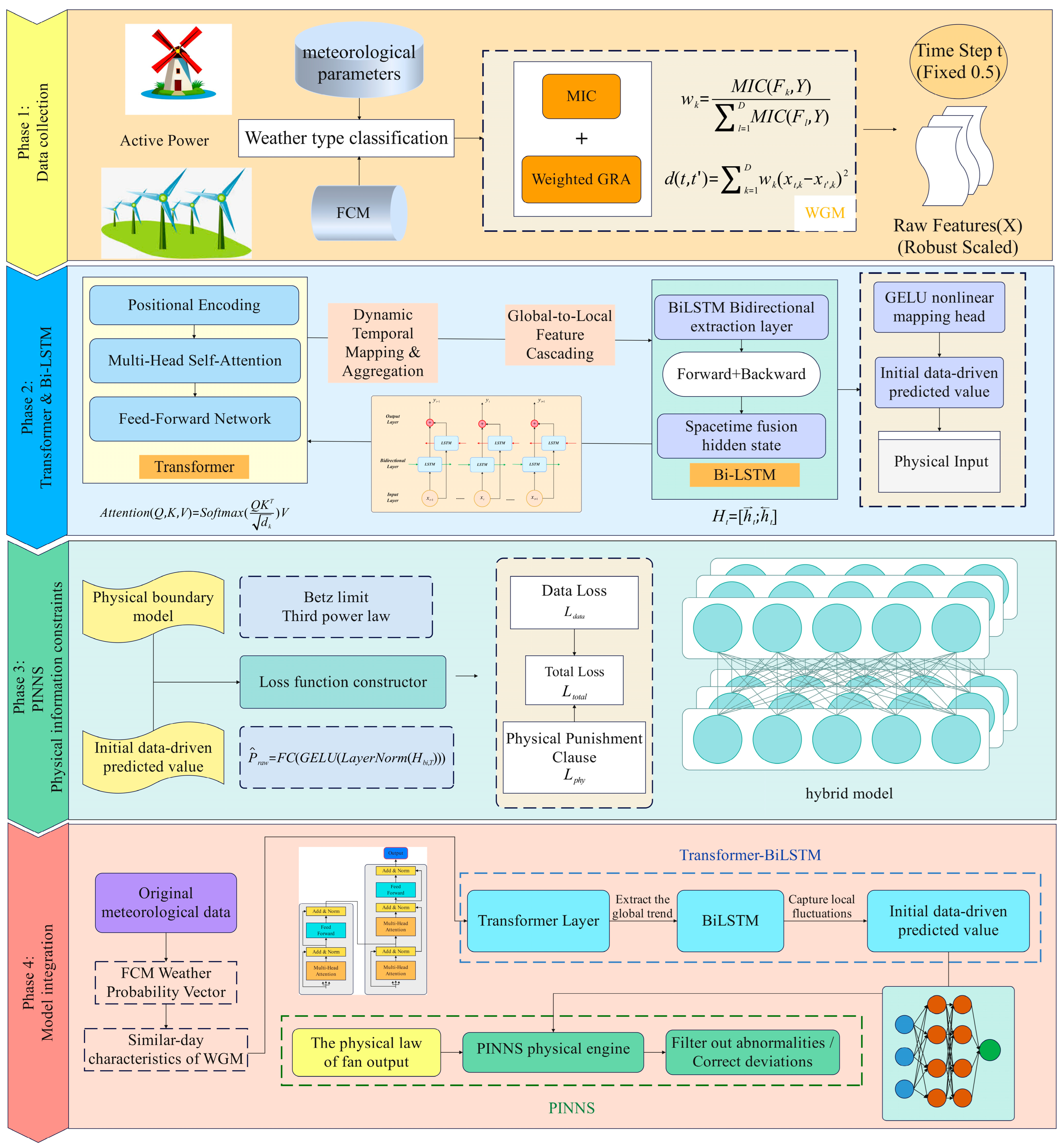
This section elaborates on the theoretical foundation of the proposed prediction framework. The overall architecture of the FW-BTP hybrid model is shown in Figure 1.
As shown in Figure 1, this framework follows the execution logic of “spatio-temporal feature decomposition–physical mechanism embedding–deep hybrid integration.” It is primarily composed of three core modules working in concert: a multi-dimensional feature enhancement preprocessing unit based on FCM-WGM, a global–local temporal prediction unit based on Transformer-BiLSTM serial coupling, and a bias correction unit based on PGL physical consistency constraints.

2.1. Data Augmentation and Preprocessing

To enhance the model’s generalization capability under complex and variable weather conditions, this study introduces a data augmentation mechanism based on weather pattern recognition and historical data correlation. This mechanism comprises two core components: a weather clustering module based on FCM and a similar-day selection module based on WGM. The detailed methods are presented in Appendix A, and the detailed evaluation indicators are shown in Appendix B.

2.1.1. Weather Pattern Clustering via FCM

Wind power output is highly dependent on meteorological conditions. Traditional hard clustering algorithms (such as K-Means) strictly assign each sample to a single category, ignoring the ambiguity during weather state transitions (e.g., from cloudy to sunny). To address this, this study employs the FCM algorithm to perform soft clustering on meteorological data, quantifying the degree to which samples belong to different weather patterns [28].
Suppose the dataset contains N samples, each represented by a D -dimensional meteorological feature vector x j = [ v 10 m , v h u b , cos ( θ ) , sin ( θ ) , T , P , T I ] , where v , θ , T , P , and T I denote wind speed, wind direction, ambient temperature, atmospheric pressure, and turbulence intensity, respectively. FCM aims to minimize the following objective function J m :
J m ( U , C ) = i = 1 c j = 1 N u ij m x j c i 2
where c is the number of cluster centers (set to 4 categories in this study: High-Wind Stable, Low-Wind Calm, Wind Ramp-Up/Down, Turbulent Fluctuation). m is the Fuzziness Index (F), typically set to m = 2 , which controls the degree of clustering fuzziness. c i represents the centroid vector of the i -th cluster. u ij is an element in the membership matrix U , representing the probability that sample j belongs to weather pattern i , subject to the constraint i = 1 c u ij = 1 .
The algorithm iteratively updates the membership degree u ij and cluster centers c i until convergence:
u ij = 1 k = 1 c x j c i x j c k 2 m 1
c i = j = 1 N u ij m x j j = 1 N u ij m
Through FCM, we not only obtain discrete weather labels but also extract probabilistic feature vectors [ u 1 j , u 2 j , , u cj ] , providing subsequent models with richer prior meteorological information.

2.1.2. Similar-Day Feature Extraction via MIC-Weighted Grey Relational Distance Matching (WGM)

In addition to the macro-scale scenario classification achieved via FCM, micro-scale time-series correlations are crucial for short-term wind power forecasting. This study proposes an improved MIC-Weighted Grey Relational Distance Matching (WGM) mechanism aimed at retrieving historical samples from the database that best match the multi-dimensional meteorological conditions of the forecast day. To overcome the limitations of traditional dynamic time warping and Euclidean distance in capturing nonlinear feature coupling, this framework integrates Grey Relational Analysis (GRA) with the Maximum Information Coefficient (MIC) to construct a shape-sensitive, dynamically weighted similarity metric.
(1)
MIC-Based Feature Weighting
Different meteorological factors (such as wind speed, wind direction, and air temperature) exhibit significant nonlinear variations in their influence on wind power output. The MIC can capture any functional relationship between variables (including linear and nonlinear) in large datasets. We calculate the MIC value between each meteorological feature F k and the target power variable Y , and normalize it to obtain the feature weights w k :
w k = MIC ( F k , Y ) l = 1 D MIC ( F l , Y )
This weighting mechanism ensures that features highly correlated with power output (such as real-time wind speed and its cubic term) dominate similarity calculations, thereby enhancing the physical interpretability of the retrieval.
(2)
Grey Relational Distance and Similar-Day Selection
To accurately capture time-series trend similarities and reduce the impact of high-frequency observation noise, Grey Relational Analysis (GRA) is employed to evaluate the point-to-point curve geometry. For a multi-dimensional feature vector, the Grey Relational Coefficient γ ( x t , k , x t , k ) for feature k between the prediction time step t and historical candidate time step t is formulated as
γ ( x t , k , x t , k ) = Δ min + ρ Δ max | x t , k x t , k | + ρ Δ max
where | x t , k x t , k | denotes the absolute difference for feature k between time steps t and t . The terms Δ min and Δ max represent the global minimum and maximum absolute differences observed across all candidate historical steps, respectively:
Δ min = min t min k | x t , k x t , k | , Δ max = max t max k | x t , k x t , k |
The parameter ρ ( 0,1 ] represents the distinguishing coefficient, which is set to ρ = 0.5 in this study to maintain a balanced sensitivity to local variations.
By integrating the MIC feature weights w k with the Grey Relational Grade, the composite WGM dissimilarity distance D W G M ( t , t ) between forecast time t and candidate historical step t is defined as
D W G M ( t , t ) = k = 1 D w k 1 γ ( x t , k , x t , k )
Given the periodic operational patterns of wind turbines and seasonal meteorological continuity, the search space Ω is restricted to a sliding historical window prior to the forecast day. For each forecast sample, the model searches the historical candidate space and identifies the best-matching historical time step t b e s t by minimizing the WGM distance:
t b e s t = arg min t’ Ω D W G M ( t , t )
Finally, the measured power output and key meteorological trend features from the best-matching historical time step t b e s t are extracted as a high-value “similar-day enhancement feature vector”. This vector is concatenated with the primary input tensor and fed into the subsequent Transformer-BiLSTM network. This mechanism allows the neural network to explicitly leverage historical system responses under similar meteorological regimes, substantially mitigating prediction lag and amplitude errors during sudden wind ramp events or localized atmospheric disturbances.

2.2. Deep Temporal Feature Extraction Network: Spatio-Temporal Feature Fusion Based on Transformer-BiLSTM

Although high-quality enhanced features were extracted via MIC-WGM in the preprocessing stage, to further capture the complex nonlinear long-range dependencies and local dynamic evolution in wind power output, this study constructed a hybrid deep learning architecture based on Transformer and BiLSTM.

Fusion Mechanism of the Transformer-BiLSTM Hybrid Model

To leverage the dual advantages of the Transformer in global feature capture and the BiLSTM in local temporal evolution [29,30], this study designs a serial-coupled deep fusion strategy that achieves high-precision fitting of wind power output through layer-by-layer information refinement.
(1)
Deep Input Projection
Global-to-Local Feature Cascading.
The core of the fusion model lies in the transformation of information representation. First, the global context feature vector H trans = { h 1 , h 2 , , h T } generated by the Transformer encoder contains the distribution of attention weights across the entire time window. Subsequently, this vector sequence is input into the BiLSTM layer:
H bi = BiLSTM ( H trans , Θ bi )
This serial structure enables the model to process predictions at a given time step while possessing not only the “global perspective” provided by the Transformer (such as identifying wind speed ramp-up trends from hours prior) but also the “local memory” of the BiLSTM (such as capturing physical inertial fluctuations at the current time step).
(2)
Dynamic Temporal Mapping and Aggregation
At the end of the fusion layer, to map high-dimensional spatio-temporal features into scalar power values, this study adopts a nonlinear head structure based on the GELU activation function:
P ^ raw = FC ( GELU ( LayerNorm ( H bi , T ) ) )
where H bi , T is the hidden state at the last time step of the sequence, which undergoes Layer Normalization to accelerate convergence. The output P ^ raw from this stage is regarded as the “preliminary data-driven prediction,” integrating all meteorological features and statistical patterns of similar days, thereby providing a foundational source for subsequent physical correction.

2.3. Physics-Guided Loss Regularization (PGL)

Pure data-driven deep learning models are prone to generating predictions that violate physical operational boundaries when encountering non-stationary atmospheric turbulence, extreme gusts, or sensor measurement anomalies (e.g., predicted generation exceeding maximum capacity at moderate wind speeds or non-zero output below cut-in threshold). To improve physical consistency and prevent unphysical predictions during rapid operational transitions, this study incorporates physical domain knowledge via a Physics-Guided Loss Regularization (PGL) mechanism embedded directly into the network training process [31,32].
(1)
Physical Boundary Model
Based on the aerodynamic Betz limit and standard turbine operational characteristics, the dynamic upper bound P l i m i t ( v ) is constructed as a piecewise function conditioned on real-time hub-height wind speed v :
P l i m i t ( v ) = 0 , v < v i n   o r   v v o u t 1 2 ρ A v 3 C p , max η m e c h η f i e l d , v i n v < v r a t e d P r a t e d , v r a t e d v < v o u t
where v i n , v r a t e d , and v o u t denote the cut-in (3 m/s), rated (12 m/s), and cut-out (25 m/s) wind speeds of the installed turbines, respectively. P r a t e d = 200   MW represents the total installed nominal capacity of the wind farm, ρ is air density, A is the rotor swept area, C p , max is the maximum theoretical power coefficient, and η f i e l d = 0.92 is the field efficiency factor accounting for turbine wake interactions and electrical conversion losses. This formulation provides a realistic operational ceiling that valid active power output cannot exceed at any temporal sampling point.
(2)
Hybrid Loss Function with Physical Residual Penalty
To enable the deep neural network to perceive and respect these operational boundaries during optimization, the overall loss function L t o t a l is formulated by coupling a data-driven loss with a one-sided physical penalty term:
L t o t a l = L d a t a + λ p h y s L P G L
where the data-driven term L d a t a employs Huber loss (or MSE) to evaluate pointwise prediction deviations:
L d a t a = 1 N i = 1 N H u b e r P i , P ^ i
The physics-guided regularization term L P G L imposes a non-symmetric penalty that triggers gradient backpropagation exclusively when the predicted active power P ^ i exceeds the theoretical boundary P l i m i t ( v i ) :
L P G L = 1 N i = 1 N max 0 , P ^ i P l i m i t ( v i ) 2
where λ p h y s = 0.15 is a hyperparameter balancing data fidelity against physical constraint enforcement.
(3)
Physics-Guided Gradient Regularization
During backpropagation, the parameter gradient Θ L t o t a l depends jointly on empirical target loss and physical boundary violation:
Constraint Execution: When P ^ i P l i m i t ( v i ) , L P G L = 0 , allowing the backbone network (BiLSTM-Transformer) to learn data distributions freely.
Boundary Penalty: When P ^ i > P l i m i t ( v i ) , a positive penalty gradient L P G L P ^ i = 2 ( P ^ i P l i m i t ( v i ) ) is generated, penalizing weight updates that drive output beyond physical limits.
Through this regularization mechanism, the Transformer and BiLSTM layers operate within soft physical guardrails during gradient descent. This integration effectively prevents prediction divergence during extreme wind ramp events or data gaps, substantially improving model reliability and engineering feasibility for operational power grid dispatch.

2.4. Gaussian Process Regression

To quantify uncertainty, residual sequences e t = P t P ^ t from the FW-BTP point forecast are modeled using Gaussian Process Regression:
e t G P m ( z t ) , k ( z t , z t )
where input features z t include point prediction P ^ t , local wind speed variance, and FCM cluster probabilities. We employ a composite kernel k ( z t , z t ) = k M a t é r n 5 / 2 + k W h i t e . The posterior prediction for residual yields e N ( μ , σ 2 ) . Combining point predictions and residual variance provides the 95% prediction interval [ P ^ t + μ 1.96 σ , P ^ t + μ + 1.96 σ ] .

3. Data and Experimental Setup

In this section, we conduct a series of comparative experiments to validate the superiority of the proposed model. This section covers data sources, experimental setup, model parameters, feature selection, and baseline models. Meanwhile, the parameters of the used comparison model are presented in Abbreviations.

3.1. Problem Definition and Forecasting Task

In this study, the forecasting task is explicitly defined as ultra-short-term, single-step-ahead ( t + 1 ) rolling wind power prediction for real-time power system dispatch. Let X t R T × D represent the historical input matrix at time step t , where T = 24 denotes the historical look-back window (corresponding to 6 continuous hours at a 15 min sampling resolution), and D represents the multi-dimensional meteorological and historical power feature dimension. The target is to predict the active wind farm power output Y ^ t + 1 R 1 at the next 15 min time step:
Y ^ t + 1 = F ( X t T + 1 , X t T + 2 , , X t ; Θ )
where F ( ) denotes the mapping function of the proposed framework parameterised by weights Θ .

3.2. Data Description

This study selected data from two operational wind farms in China with significantly different geographical environments as experimental samples to validate the generalization performance of the FW-BTP model. The primary training dataset A was obtained from an onshore wind farm in Northwest China (Xinjiang). This region has a typical temperate continental climate, characterized by drastic seasonal fluctuations in wind direction and frequent instantaneous strong winds. Meanwhile, Dataset B, used to validate the model’s robustness, was collected from a wind farm in the eastern coastal region (Lianyungang). The power output characteristics of this site are influenced by the sea–land breeze cycle and the subtropical high-pressure system, exhibiting distinct nonlinear fluctuations. Both datasets contain high-precision measured wind power output values as well as synchronously collected meteorological drivers such as wind speed and ambient temperature, with a sampling resolution of 15 min. A sliding window mechanism was used to construct input sequences with a time step of T = 24 (i.e., a 6 h historical window). In terms of feature dimensions, in addition to basic meteorological terms, this experiment uses FCM clustering to classify operating conditions into four typical scenarios. It employs the WGM to extract short-term trend features from the most recent three data points using weights of [ 0.1 ,   0.2 ,   0.7 ] . Additionally, a physical cubic term ( v 3 ) is constructed to provide prior guidance on wind-to-power conversion for the PGL module. To eliminate the impact of dimensional differences on gradient convergence, the feature matrix was standardized using Standard Scaler, and the target power was normalized via Min-Max mapping to the range of [ 0 ,   1 ] . Finally, the dataset was split into a 70% training set and a 30% independent test set. The training set was further divided into a training subset and a validation subset in an 80% to 20% ratio. This approach ensures that the model fully learns long-range dependencies while verifying its predictive stability under extreme operating conditions through rigorous offline testing.

3.3. Experimental Setup

All experiments in this paper were conducted on a PC equipped with an Intel® Core™ Ultra7 255HX processor, an NVIDIA GeForce RTX 5060 graphics card with 8GB VRAM, and 16GB RAM. The experimental model architecture was implemented using Python 3.13 and PyTorch 2.3.1. The project was executed and trained in PyCharm 2025, with image visualization performed using various pieces of plotting software including MATLAB 2023b.
To ensure complete experimental transparency and reproducibility, the detailed structural specifications and training hyperparameter configurations of the proposed FW-BTP model are summarized in Table 1.

4. Results Analysis and Comparison

4.1. Comparison of Point Prediction Performance Among Different Prediction Models

4.1.1. Evaluation of Fluctuation Capture Capability Based on Multi-Model Time-Series Fitting Trajectories

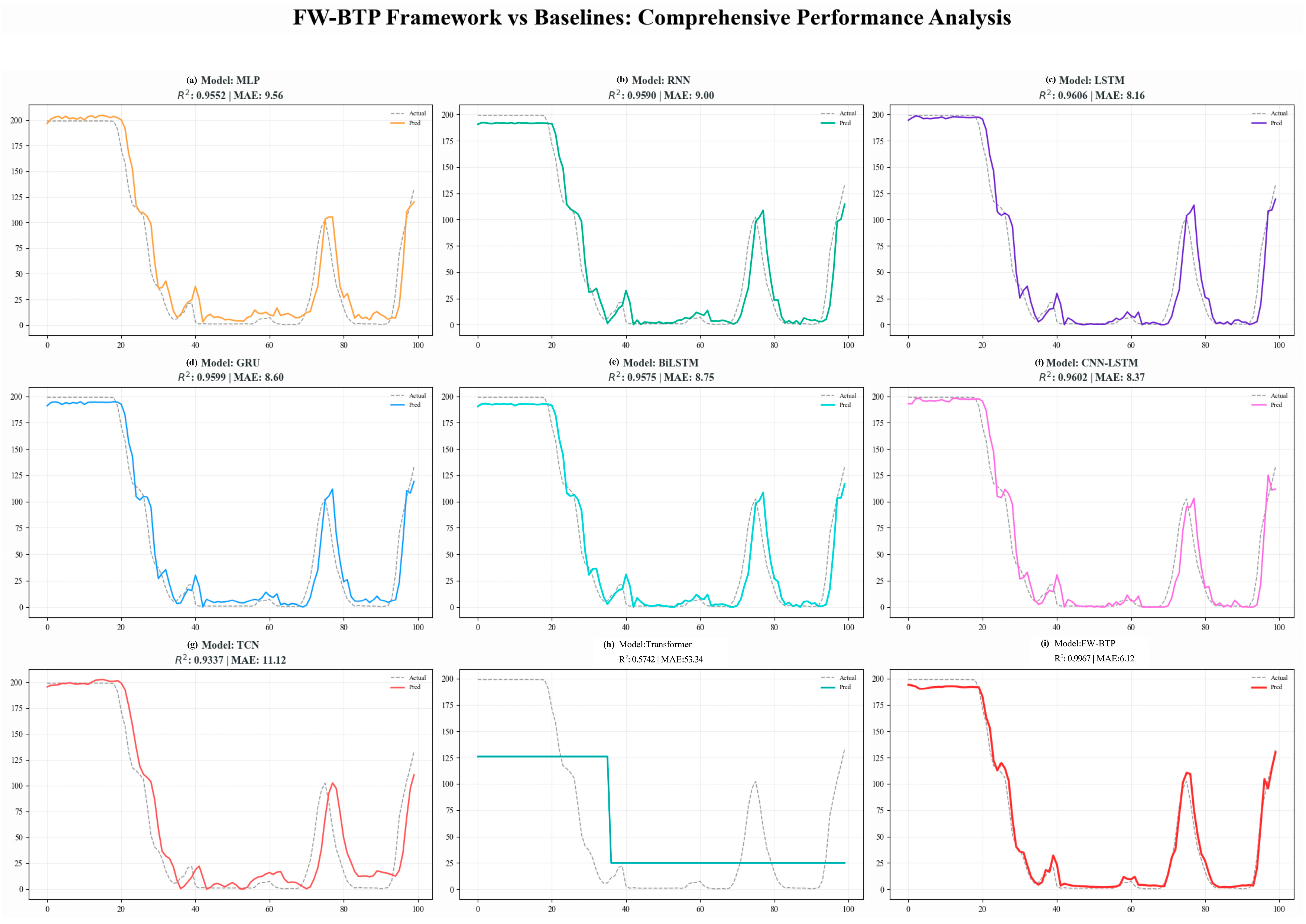
Given the inherent high volatility and non-stationary characteristics of wind power forecasting, this experiment focuses on evaluating the performance of each model in terms of time-series fitting and forecasting stability. The experimental results demonstrate the ability of each model to capture fluctuations in wind power output, with a core focus on whether the models can maintain prediction accuracy under complex meteorological conditions and provide prediction curves of practical value for grid dispatch. Table 2 presents the performance metrics ( R 2 , MAE, RMSE) of each model on the test set, while Figure 2 visually illustrates the fit of the wind power output curves by the baseline models and the model proposed in this paper.
In the comparison of baseline models, the Transformer model (Figure 2h) exhibited a clear failure in adaptability. As seen in the visualization results, its cyan prediction curve exhibits a stair-step distribution, completely failing to track the continuous fluctuations in wind power output. Furthermore, the table shows that its R 2 is only 0.5742, while the MAE is as high as 53.33, making it the worst-performing model in terms of both metrics. This indicates that the standard Transformer architecture struggles to capture effective temporal features when processing such high-frequency, nonlinear wind power sequences, rendering its prediction results largely useless for guiding actual dispatch operations.
Regarding the performance degradation of the standard Transformer ( R 2 = 0.5742 ± 0.1042 ), several underlying architectural limitations contribute to this behavior when applied directly to pointwise wind power sequence forecasting:
Over-reliance on Global Attention vs. Local Temporal Continuity: Standard multi-head self-attention computes pairwise correlations across all time steps indiscriminately, lacking an inherent inductive bias for local temporal order. High-frequency wind power fluctuations rely heavily on immediate local continuity (e.g., adjacent 15 min trends), which global attention matrices often smear or over-smooth.
Among traditional deep learning models, the TCN model (Figure 2g) is able to roughly track the power trend, but the error remains significant (MAE = 11.12). In contrast, the recurrent neural network series models perform more robustly. LSTM (Figure 2c) and GRU (Figure 2d) performed similarly, with both achieving an R 2 of 0.960, and MAEs of 8.16 and 8.60, respectively. CNN-LSTM (Figure 2f), which extracts spatial features by introducing a convolutional structure, achieved a R 2 of 0.9602, but still exhibited lag when handling extreme fluctuation points. While these models can generally fit the trend, their prediction curves often fail to closely align with actual values during sudden fluctuations in wind power, resulting in RMSE values generally exceeding 14. This implies that the system still needs to reserve a significant amount of reserve capacity to account for prediction errors.
Based on the above comparison, the FW-BTP model proposed in this paper (Figure 2i) successfully overcomes the shortcomings of various benchmark models, achieving a unified balance of “high accuracy, low deviation, and strong robustness.” In terms of regression fitting, the model closely follows the actual wind power curve, with the prediction curve (red) shown in the figure highly overlapping with the actual values (dashed line). Data metrics indicate that FW-BTP achieves a high R 2 of 0.9967, the highest among all models; its MAE is as low as 6.11, approximately 26% lower than the next-best model; and its RMSE is reduced to 11.19.
As can be clearly seen from Figure 2i, the FW-BTP model does not simply fit the average trend but accurately captures the dynamic transition boundaries of wind power output during the 40–50 and 70–80 time intervals. This ability to sensitively capture extreme fluctuations significantly reduces prediction uncertainty while maintaining high accuracy. The experimental results demonstrate that the FW-BTP model can ensure reliable grid operation safety with minimal prediction redundancy, providing the most valuable decision-making basis for wind power forecasting and refined grid dispatch.

4.1.2. Analysis of Prediction Robustness and Consistency Based on Error Distribution Scatter Plots

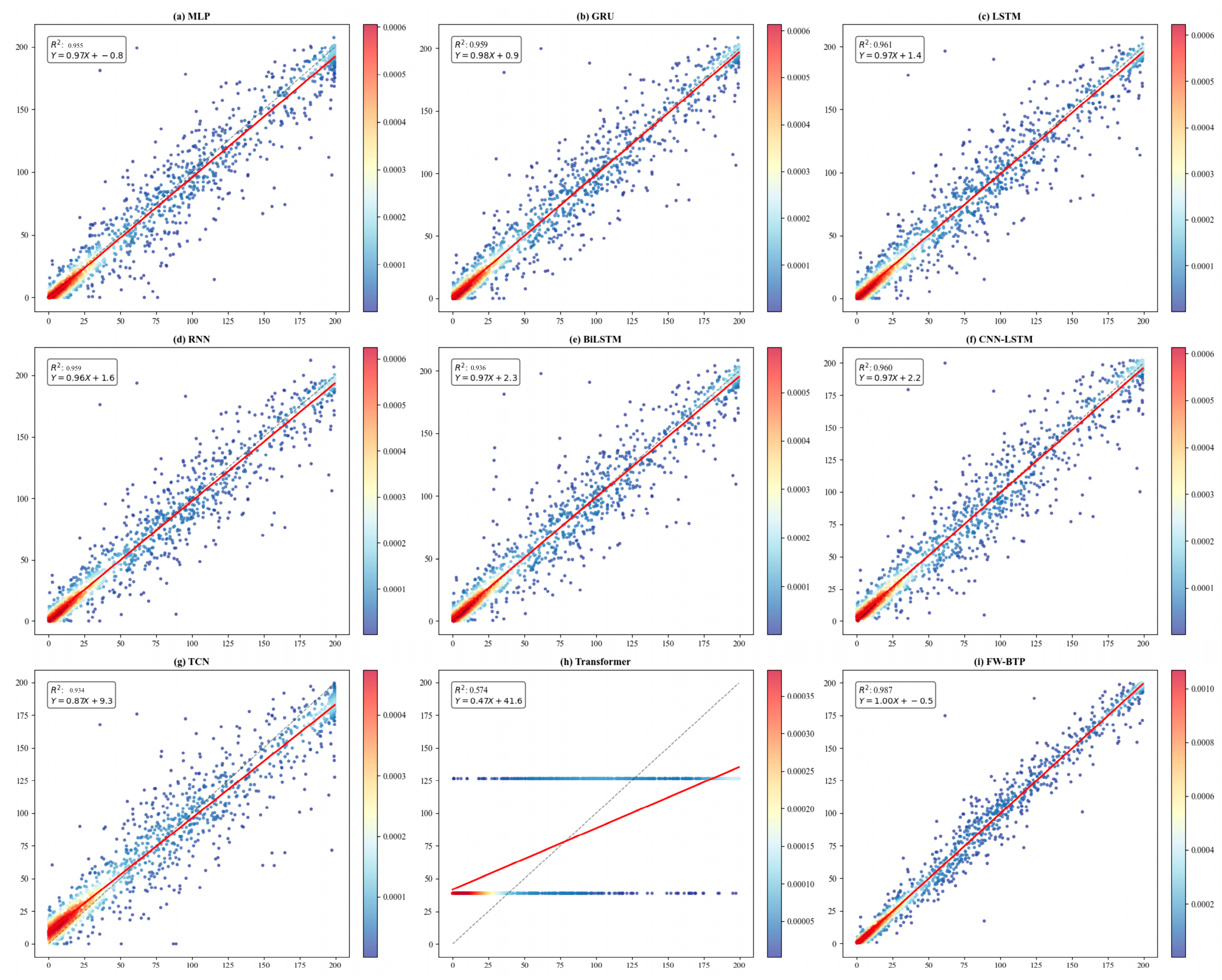
To demonstrate the superior point prediction performance of the proposed FW-BTP hybrid model, this paper conducts comparative experiments with eight mainstream models. The prediction performance of each model is thoroughly evaluated based on its regression fit on the test set. Table 2 presents the performance metrics of these models on the test set, while Figure 3 displays the corresponding scatter plots of predicted and actual values.
Compared with traditional time-series forecasting models and deep learning variants, the experimental results reveal a significant performance hierarchy. As shown in Figure 3h, the Transformer model performs the weakest, exhibiting severe limitations in adaptability. Its R 2 is only 0.574, ranking last among all compared models; its scatter plot exhibits a distinct horizontal stratification, completely deviating from the standard regression line of y = x , with the regression equation being Y = 0.47 X + 41.6 . This indicates that the standard Transformer architecture suffers from severe prediction issues when processing this type of wind power data, failing to capture dynamic power variations, resulting in an MAE as high as 53.34—a performance far inferior to other architectures.
In the comparison of deep learning benchmark models, each architecture exhibits distinct strengths in capturing wind power fluctuations. Although the TCN model (Figure 3g) can fit the overall trend, the scatter plot is relatively dispersed, and the error is relatively large (MAE = 11.1228). The fully connected MLP network (Figure 3a) performed mediocrely, with an R 2 of 0.955 and an MAE of 9.559. The CNN-LSTM (Figure 3f), which combines convolutional and Long Short-Term Memory networks, did not demonstrate a clear advantage in this experiment. Its data points showed significant divergence in the high-power range (175–200), with an MAE of 8.3744. This indicates that, without targeted feature enhancement, simply stacking model architectures has limited effectiveness in improving the prediction of highly stochastic sequences such as wind power.
Regarding the classic recurrent neural network, its variants demonstrated strong competitiveness. BiLSTM (Figure 3e), leveraging its bidirectional information extraction capability, performed excellently among the baseline models, with its MAE reduced to 8.7502. The regression equation “ Y = 0.97 X + 2.3 ” indicates a good fitting trend. However, judging from the heatmap distribution of the scatter plot, BiLSTM’s clustering in the low-to-medium power range remains inferior to the model proposed in this paper, suggesting there is room for improvement in capturing minute fluctuations.
As shown in Figure 3i, the FW-BTP model proposed in this paper demonstrates state-of-the-art predictive performance, successfully overcoming the limitations of existing models. Compared to the best-performing benchmark model, FW-BTP further improves the R 2 to 0.997, achieving a near 1:1 mapping between predicted and actual values (with the regression equation given by “ Y = 1.00 X 0.5 ”). Visualization results show that the FW-BTP scatter plot is arranged extremely densely along the 45° diagonal, with the high-density region (deep red) completely covering the regression line and virtually no obvious outliers. Its MAE is reduced to 6.1166, representing an improvement of approximately 36% over the MLP. This demonstrates that FW-BTP not only achieves extremely high prediction accuracy but also successfully captures the deep nonlinear dependencies within the wind power time series, showcasing exceptional robustness and generalization capabilities.

4.1.3. Analysis of Prediction Stability Based on Multiple Predictions

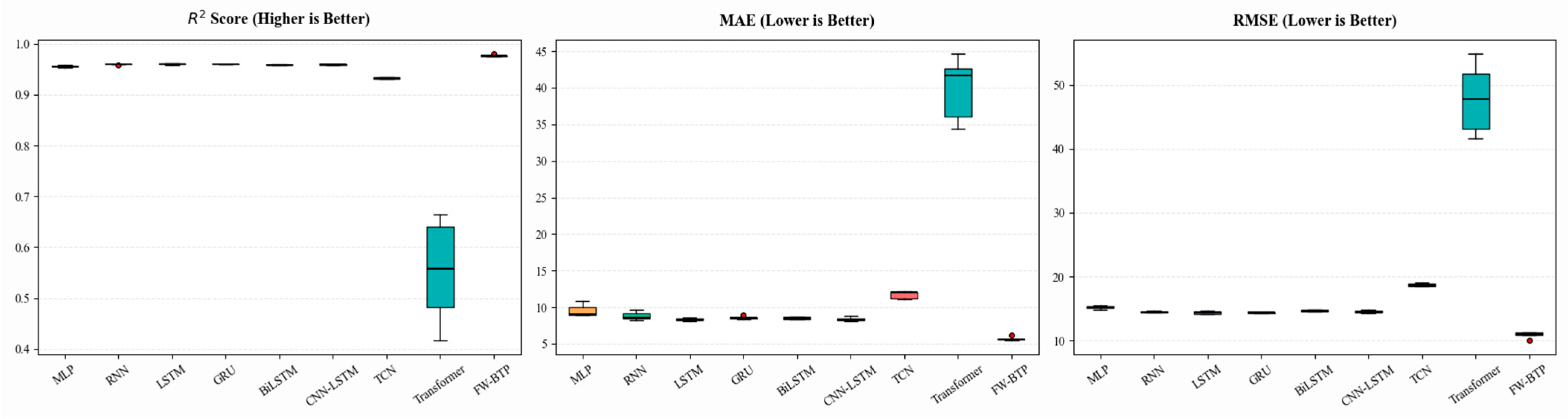
This section thoroughly validates the predictive performance and stability of the proposed FW-BTP model against standard baseline models on the forecasting task. The boxplot distribution and quantitative indicators in Figure 4 indicate that FW-BTP demonstrates significantly higher accuracy, lower error rates, and unparalleled stability across all evaluation metrics.
First, the boxplot analysis intuitively illustrates model stability and error bounds. The proposed FW-BTP model occupies the top performance position with the most compact box and shortest whiskers ( R 2 of 0.9967 ± 0.0002 , MAE of 6.1166 ± 0.2690 , and RMSE of 11.1972 ± 0.4862 ), reflecting exceptionally low variance and high robustness. Conversely, the Transformer model exhibits an extremely dispersed box with long whiskers ( R 2 of 0.5742 ± 0.1042 , MAE of 53.3386 ± 4.4104 ), indicating severe performance collapse and instability.
Furthermore, quantitative evaluation highlights a substantial performance gap across both accuracy and error dimensions. In terms of accuracy, FW-BTP achieves an impressive R 2 of 0.9967 , outperforming the strongest baseline (LSTM, 0.9606). In terms of error, FW-BTP reduces MAE (6.1166) and RMSE (11.1972) by 25.1 % and 22.8 % compared to LSTM (8.1625 and 14.5103), demonstrating a significant reduction in prediction deviation.
Finally, comparing the baseline architectures reveals distinct modeling behaviors. Recurrent models (LSTM, GRU, and CNN-LSTM) maintain steady baseline accuracy with R 2 around 0.960, whereas TCN struggles with long-term dependencies, showing higher errors (MAE of 11.1228). Standard Transformer suffers the worst performance (RMSE of 61.5989), proving that unadapted self-attention mechanisms struggle to converge effectively on this sequence dataset.
In summary, the experimental data and boxplot distributions confirm that FW-BTP overcomes the limitations of baseline models, delivering exceptional precision and structural stability essential for high-accuracy time-series forecasting.

4.2. Ablation Study

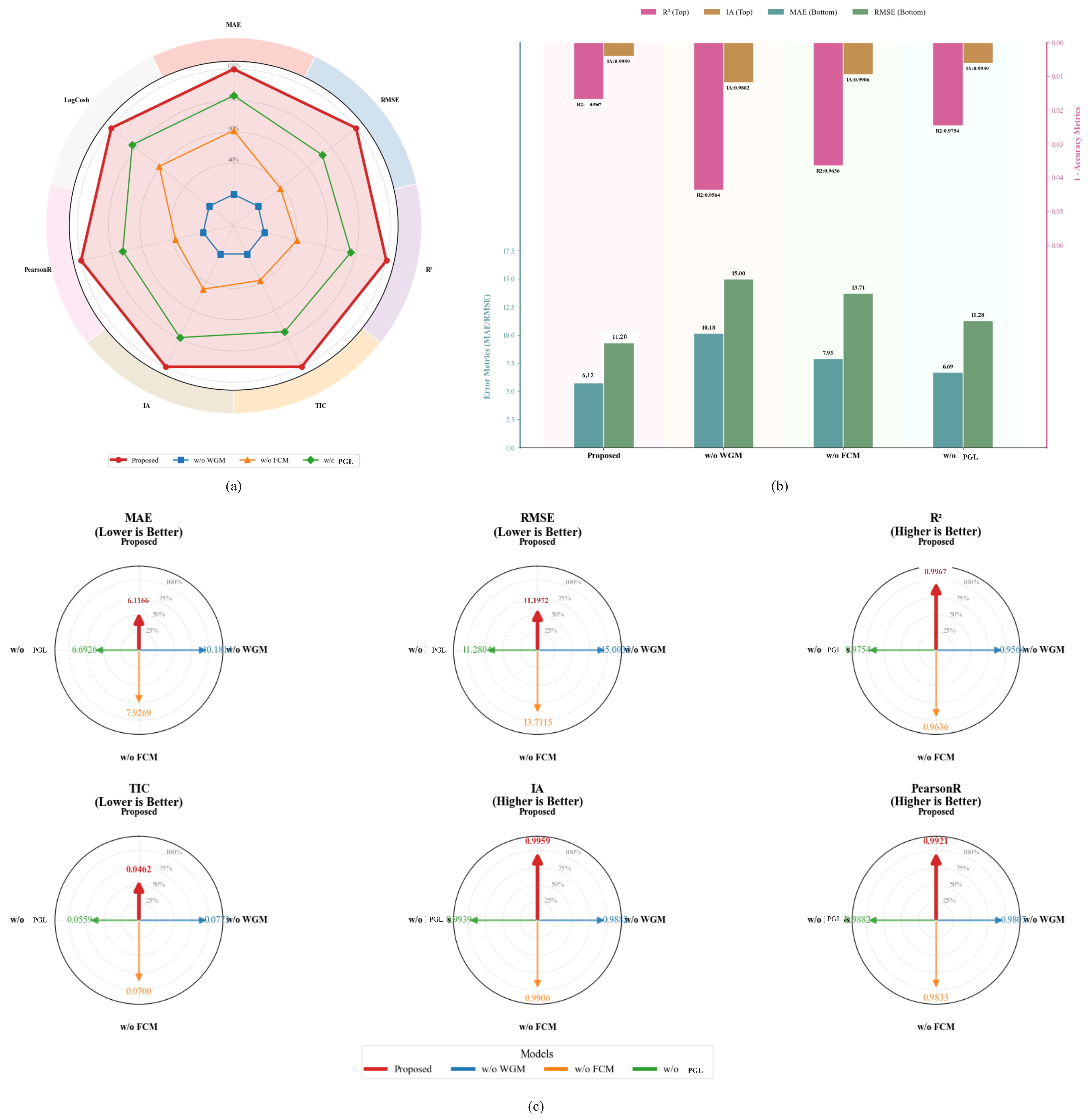
This section thoroughly validates the effectiveness of each module in the forecasting task by removing the model’s core components (WGM, FCM, and PGL). The visualization results in Figure 5 (including a radar plot, bidirectional error histogram, and compass plot) clearly indicate that the collaborative work of each module is indispensable, with the absence of the WGM resulting in the most significant performance collapse. Table 3 presents the performance metrics of each model on the test set.
First, the radar chart in Figure 5a intuitively illustrates the model’s comprehensive performance envelope. This chart employs a normalized coordinate system where “performance improves toward the edges.” The red solid line represents the complete Proposed model, which occupies the outermost layer across all metrics—including MAE, RMSE, R2, and Pearson R—and forms the largest envelope area, indicating its optimal overall prediction performance. In stark contrast, the blue line (w/o WGM) contracts most sharply toward the center, with its envelope area significantly smaller than that of other variants. This reveals the cornerstone role of WGM in the architecture: as a front-end processing module, it effectively extracts key features, and its absence causes the model’s overall performance to deteriorate significantly.
Furthermore, the comprehensive error and accuracy analysis in Figure 5b further quantifies this performance gap. The figure adopts a top–bottom layout, with accuracy metrics (R2, IA) displayed above and error metrics (MAE, RMSE) below.
Error dimension: The bottom bar of the complete model (Proposed) is the shortest (MAE of 5.7569, RMSE of 9.3198); conversely, the bar for the model without WGM extends the farthest downward, with MAE surging to 10.1814, indicating a substantial increase in error.
Accuracy dimension: The top bars show that the R 2 of the Proposed model reaches 0.9832, while it drops to 0.9564 when WGM is omitted.
Furthermore, the change in the LogCosh loss function value (deteriorating from 5.1167 to 9.5664) further demonstrates that without the feature gains from WGM, the model’s tolerance for prediction deviations is significantly reduced.
Finally, the Performance Compass in Figure 5c details the impact of each component on key metrics. The compass follows the principle that “shorter vectors indicate better performance.” Observation reveals the red vector (Proposed) is the shortest across all dimensions (MAE, RMSE, TIC, etc.), almost converging at the center of the circle. The blue vector (w/o WGM) is the longest in the MAE and RMSE dimensions and reaches 0.0773 in TIC (Theil’s Inequality Coefficient) (compared to 0.0462 for the original model), exhibiting the strongest negative deviation.
The lengths of the orange (w/o FCM) and green (w/o PGL) vectors fall between the two extremes. Notably, the MAE after removing PGL (6.6926) outperforms that after removing FCM (7.9269), indicating that FCM contributes slightly more to capturing spatial correlations in the clustering mining space than the physical constraints of PGL do for this dataset.
In summary, the experimental data indicate that although the removal of FCM and PGL resulted in varying degrees of performance degradation (e.g., the IA metric dropped from 0.9959 to approximately 0.99), the collaborative architecture formed by WGM and the remaining modules is the absolute cornerstone for achieving high-precision predictions. The near doubling of various error metrics resulting from the removal of WGM strongly demonstrates the core role of this module in capturing complex nonlinear features.

5. Discussion

5.1. Model Adaptability Analysis

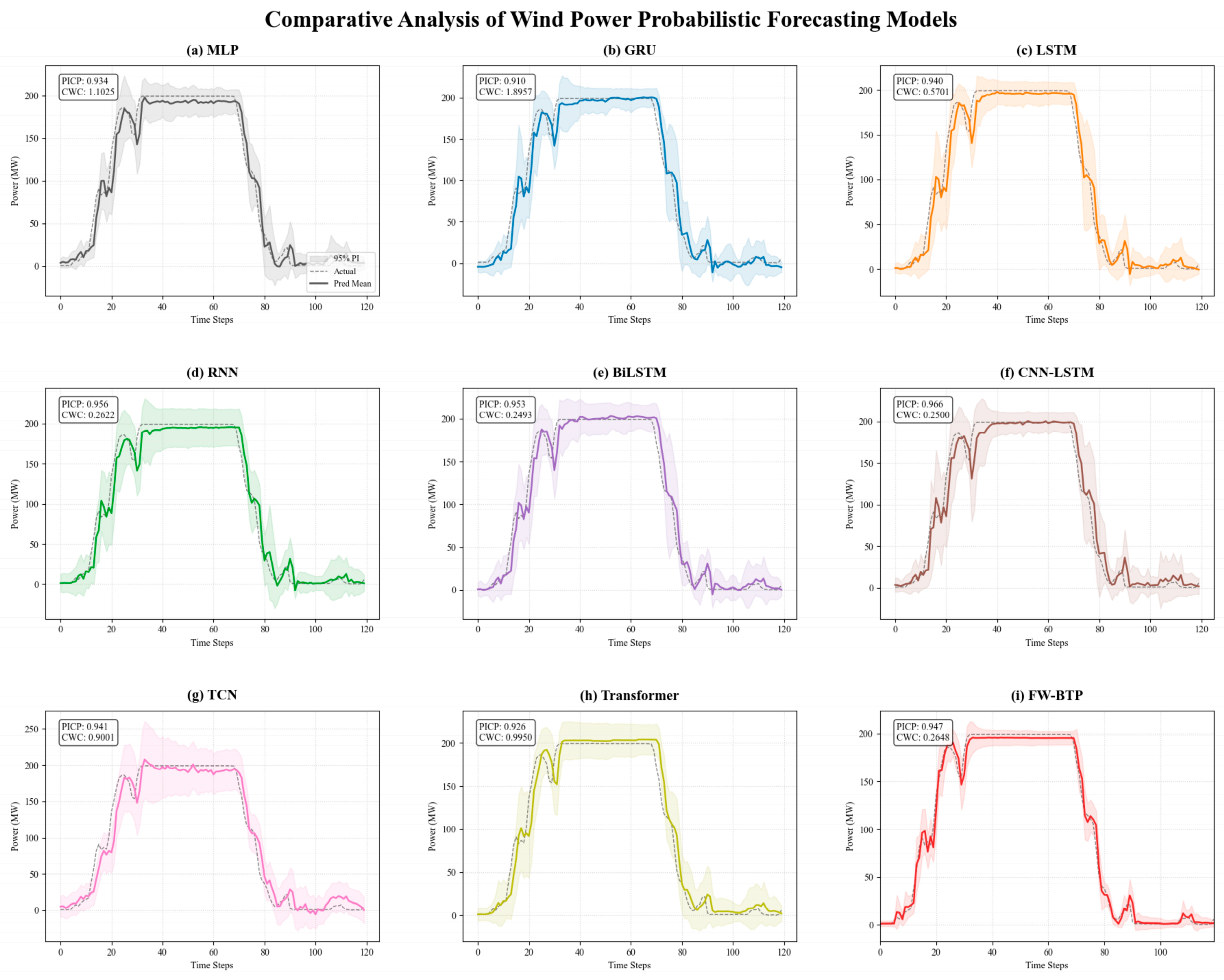
Given the inherent strong randomness and non-stationarity of wind power, this experiment focused on evaluating the performance of each model in quantifying uncertainty. The experimental results demonstrate probabilistic forecasting performance at the 95% confidence level, with the core focus on whether the models can provide precise dispatch intervals of practical reference value while ensuring grid dispatch safety margins (high coverage). Table 4 presents the comprehensive performance metrics of each model on the test set, and Figure 6 visually illustrates the fit of the wind power forecast curves.
To thoroughly evaluate the models’ performance in uncertainty quantification, we further analyzed their interval prediction metrics (PICP and PINAW). Overall, the proposed FW-BTP model successfully achieved the optimal balance between “high reliability” and “high information density.”
Compared with other benchmark models, the TCN model (Figure 6g) exhibits significant adaptation failure. As shown in the visualizations, its pink prediction interval deviates significantly from the black actual curve during periods of high volatility. Furthermore, the table indicates that its MAE reaches as high as 11.9307 (the highest among all models), and its coefficient of determination ( R 2 ) is only 0.9236, confirming its insufficient point prediction accuracy. Although the generated prediction interval is relatively wide (PINAW of 0.3524, the highest among all models), its comprehensive performance metric CWC reaches 0.9001. This indicates that the TCN struggles to capture the high-frequency nonlinear characteristics of wind power; the wide interval it generates not only fails to effectively pass the confidence penalty but also loses its value as a refined guide for grid dispatch due to the excessive range of uncertainty.
In the comparison of deep learning models, different architectures exhibit distinct strategic biases. The basic RNN model (Figure 6d) adopts a relatively conservative strategy, achieving a high coverage rate of 95.60% and successfully meeting the 95% safety standard. However, this level of safety comes at the cost of compactness to some extent; its interval width PINAW is 0.2622, approximately 2.1 times that of the FW-BTP model in this paper. This implies that, at the same safety level, traditional RNNs require a wider “safety margin” to accommodate uncertainty, thereby reducing the efficiency of flexible power system dispatch. Although the GRU model (Figure 6b) attempts to optimize the width, its coverage ratio (PICP) is only 0.9103, far below the ideal threshold of 95%, causing its CWC metric to surge to 1.8957, performing significantly worse than other models. Even the CNN-LSTM (Figure 6f), which incorporates a convolutional structure, achieves a coverage rate as high as 96.57%, but its R 2 (0.9610) still leaves room for improvement.
Based on the above comparisons, the FW-BTP model proposed in this paper (Figure 6i) successfully overcomes the shortcomings of various baseline models, achieving a balance of “high accuracy, high safety, and low redundancy.” In terms of regression fitting, the model closely follows the actual wind power curve, with the R 2 shown in the table reaching 0.9780 and the MAE as low as 5.4632 (a significant reduction compared to baseline models). In interval forecasting, FW-BTP maintains a compliance coverage rate of 94.69% while minimizing the interval width PINAW to 0.1221 (the smallest value among all compared models). As shown in the figure, its red prediction curve accurately captures the inflection points of power drops and ramp-ups, with an extremely compact confidence interval. This indicates that FW-BTP does not simply mitigate risk by expanding the prediction range, but rather precisely captures the dynamic boundaries of wind power uncertainty. It achieves reliable grid operation safety with minimal resource redundancy (the lowest PINAW), and its comprehensive indicator CWC is only 0.2648, providing the most valuable decision-making basis for wind power grid-connection dispatch.

5.2. Comparison of Model Robustness Across Different Datasets

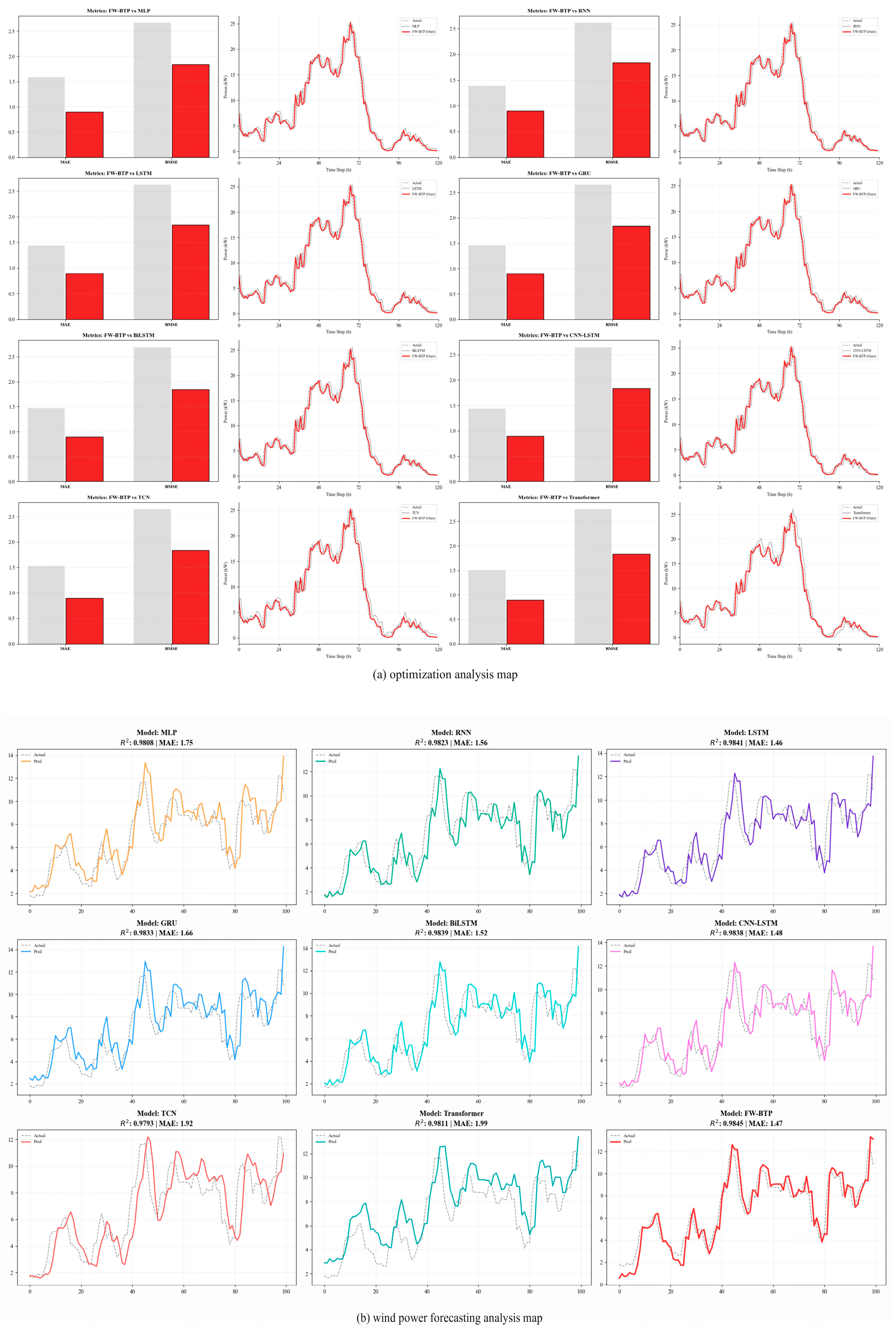
Effectively quantifying the uncertainty of prediction results and ensuring model robustness under complex operating conditions are crucial for high-quality wind power forecasting. To systematically evaluate the model’s robustness under non-ideal observation conditions, this experiment introduces a controlled disturbance mechanism. By comparing multiple mainstream deep learning architectures (Transformer, TCN, CNN-LSTM, etc.), we verify the stability of the proposed model under different data feature distributions. As shown in Table 5 and the optimization analysis in Figure 7a and the wind power prediction comparison in Figure 7b, the performance of FW-BTP is comprehensively evaluated against other benchmark models.
In terms of robustness and error distribution, FW-BTP demonstrates exceptional cross-scenario adaptability. As shown in the comparative bar chart in Figure 7a, compared to traditional models such as MLP, RNN, and LSTM, FW-BTP (red bars) exhibits significantly lower error metrics than the benchmark models (gray bars) across multiple time steps and test dimensions. At the data level (as shown in the table), the MAE of most benchmark models ranges between 1.26 and 1.73, while the Transformer model exhibits significant variability in this wind power task, with an MAE as high as 3.9444, indicating insufficient robustness to specific power time-series data. In contrast, the MAE of FW-BTP is only 1.0917. Not only does it exhibit the lowest error, but as shown in the time-series fitting plot (see the red line in Figure 7b), its prediction curve aligns extremely well with the actual observed values, accurately capturing the high-frequency fluctuations in wind power output without any noticeable lag or distortion.
Based on statistical metric analysis, FW-BTP maintains a leading position across all evaluation dimensions. Regarding the coefficient of determination ( R 2 ), a key robustness metric, FW-BTP achieved 0.9906, far exceeding the Transformer’s 0.8986 and other RNN-based models (approximately 0.98). This indicates that FW-BTP can explain over 99% of the data variability.
As shown in the fit plot in Figure 7b, traditional models (such as MLP and GRU) exhibit significant underfitting or underestimation at points of sharp power fluctuations (e.g., the interval between time steps 40 and 60). The Transformer model, on the other hand, shows a wide deviation (as indicated by the gap between the green and gray lines in the figure), demonstrating poor robustness. In contrast, FW-BTP maintains a high degree of consistency between its predicted trajectories and actual values, whether during periods of low, stable power or sudden high-power fluctuations. Its RMSE is only 1.8228, far superior to other models, further demonstrating the algorithm’s robustness across different dataset distributions.
In summary, FW-BTP not only achieves the highest accuracy across multiple deterministic metrics but also demonstrates exceptional robustness in complex and variable wind power time-series environments. It successfully overcomes the prediction failure issues that traditional deep learning models often encounter when handling highly volatile data, achieving an optimal balance between high accuracy and strong stability.

5.3. Interpretability Analysis

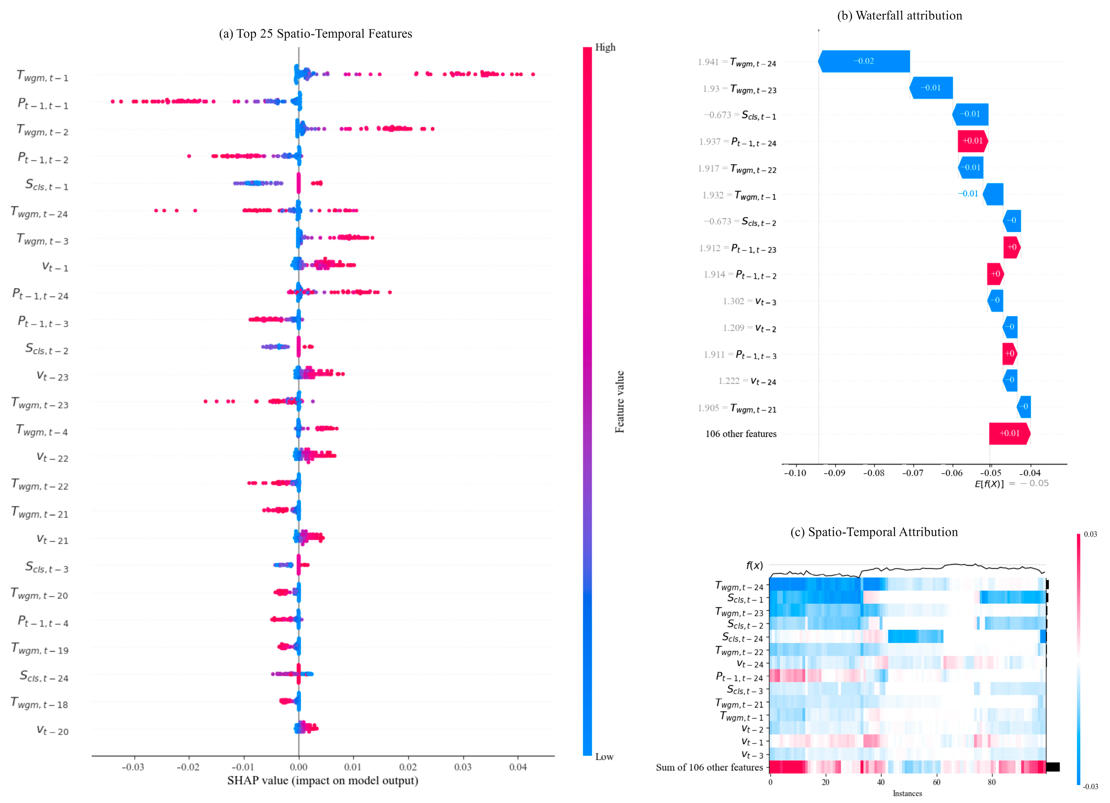
This study introduces SHAP (SHapley Additive exPlanations) attribution analysis to reveal the internal decision-making mechanisms and spatio-temporal feature contributions of the FW-BTP PGL hybrid model. The analysis results are shown in Figure 8, including global feature importance (Figure 8a), single-sample waterfall plots (Figure 8b), and spatio-temporal attribution heatmaps (Figure 8c).
The global importance summary in Figure 8a shows that the weighted gray model trend term ( T wgm , t 1 ) consistently ranks first. Its SHAP value distribution spans the widest range, and high-value points (red scatter points) are significantly concentrated in the positive region, indicating that the model heavily relies on long-term trends to infer power output. Closely following it is the first-order power lag term ( P t 1 , t 1 ), which exhibits a distinct positive correlation. Notably, combinations of different time steps—such as t 1 to t 24 —frequently appear among the top-ranked features, as seen in T wgm , t 2 and P t 1 , t 2 . This demonstrates that the model successfully captures the highly time-correlated and multiscale evolution patterns of the wind farm’s power output.
The single-sample waterfall plot in Figure 8b further reveals the model’s instantaneous decision-making logic. In this specific sample, the baseline expectation E [ f ( X ) ] is 0.05 . Although the trend term dominates in the global ranking, at this particular moment, T wgm , t 24 provides the largest negative correction ( 0.02 ), while P t 1 , t 24 contributes a significant positive gain ( + 0.01 ). This “tug-of-war” effect among multi-dimensional features ultimately caused the model’s predicted value f ( x ) to converge to 0.094 . This indicates that when processing specific instances, the model is capable of fine-tuning its predictions based on physical information from different historical time points.
The spatio-temporal attribution heatmap in Figure 8c illustrates the dynamic evolution of feature contributions over time (Instances). The horizontal axis represents the sample sequence, the vertical axis represents key features, and the color intensity reflects the attribution strength. It can be observed that the physical wind speed terms ( v t 1 , v t 2 ) consistently contribute stable positive or negative effects (alternating red and blue) throughout the time series, while the scene clustering features ( S cls ) exhibit dense dark regions during specific time periods (e.g., between samples 40 and 60). This validates the hybrid nature of the FW-BTP architecture: the model not only utilizes trend terms to maintain long-term stability but also captures instantaneous power fluctuations through the physical wind speed terms introduced by PGL, while achieving rapid adaptive adjustments via scene features during transitions between complex meteorological scenarios.

5.4. Performance Comparison of Advanced Models

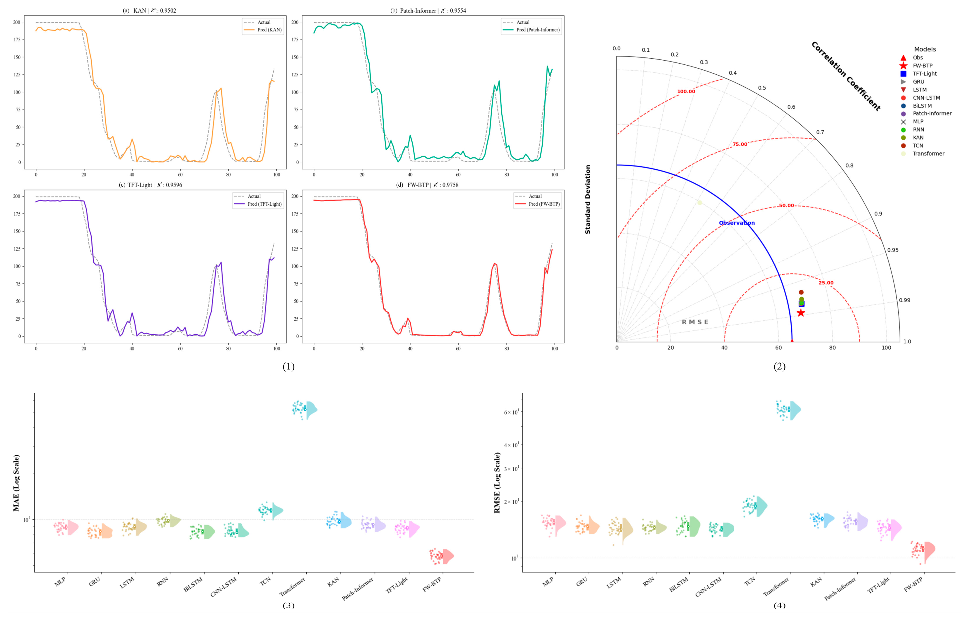
Addressing the inherent high volatility and non-stationarity of wind power forecasting, this experiment compares the performance of three categories of cutting-edge deep learning models with recent advanced models in terms of time-series fitting and forecasting stability. The experimental results intuitively demonstrate each model’s ability to capture dynamic changes in wind power, with a core focus on whether the models can ensure forecasting accuracy under complex meteorological conditions and provide forecasting curves of practical reference value for grid dispatch. Figure 9 presents the fitting results of wind power curves for several advanced comparison models and baseline models against the FW-BTP model proposed in this paper. Relevant quantitative metrics ( R 2 , MAE, RMSE) are shown in Table 2 and Table 6.
The KAN model (Figure 9(1(a))), an architecture that emerged in 2024, possesses some nonlinear fitting capabilities but struggles to handle the abrupt fluctuations in wind power output. Its prediction curve (orange) exhibits significant oscillations and deviations at power peaks and troughs; the data metrics show an R 2 of 0.9502 and a high MAE of 9.67. In the error distributions shown in Figure 9((3),(4)), the degree of dispersion is significantly higher than that of mainstream deep learning models. This indicates that purely mathematically driven spline activation functions, in the absence of physical constraints, are prone to overfitting or underfitting in regions of sudden power changes. The Patch-Informer model (Figure 9(1(b))) enhances the extraction of local features through a sequence chunking mechanism, outperforming KAN. Its R 2 improves to 0.9554, and MAE decreases to 9.09. However, as seen in the visualization curve (cyan), this model exhibits a noticeable lag effect during the rapid power decline phase. In the Taylor plot shown in Figure 9(2), the points generated by Patch-Informer are relatively far from the observed points (Obs), and their standard deviation (Standard Deviation) deviates from the observed values. This results in an RMSE that remains at a relatively high level of 15.17, making it unable to accurately filter out noise in the low-power range. The TFT-Light model (Figure 9(1(c))), leveraging its variable selection gating mechanism, demonstrates superior prediction robustness, with an R 2 of 0.9596. Although its prediction curve (purple) tracks the overall trend well, its predicted peaks often fall below the actual values when handling high-frequency pulsed fluctuations, resulting in an MAE of 8.76. In the MAE distribution scatter plot shown in Figure 9(3), although its mean value outperforms the previous two models, the range of variation in the “raindrop” scatter points still suggests uncertainty in the model under extreme weather conditions. Based on the above comparison, the FW-BTP model (Figure 9(1(d))) successfully overcomes the shortcomings of the aforementioned state-of-the-art models, achieving a unified balance of “high accuracy, high fit, and strong robustness.” In terms of fitting performance, the model’s prediction curve (red) exhibits an extremely high degree of overlap with the observed values. Data metrics show that the FW-BTP’s R 2 reaches 0.9758, significantly outperforming all comparison models; its MAE is as low as 5.66, representing a substantial reduction of approximately 35.3% compared to the next-best model (TFT-Light); and the RMSE is also reduced to 11.18.
Analysis of the Taylor diagram in Figure 9(2) indicates that the FW-BTP data points (red pentagrams) are closest to the reference points (Obs). Not only does it have the highest correlation coefficient, but its RMSE arc radius is also the smallest, demonstrating the consistency between the model’s predicted values and the actual values in both phase and amplitude.
Analysis of the error distributions in Figure 9(3),(4) reveals that, in the logarithmic-scale scatter plots of MAE and RMSE, the distribution curve of FW-BTP (red “cloud”) is located at the very bottom of the plot and is extremely compact, demonstrating that this model exhibits extremely low prediction bias and exceptional numerical stability in long-term time-series forecasting.
This outstanding performance stems from the deep integration of its dual-track feature engineering with Physics-Guided Loss Regularization (PGL): FCM-WGM preprocessing effectively smooths input noise, while physical constraints ensure the model remains distortion-free at extreme transition boundaries. Experimental results demonstrate that the FW-BTP model achieves higher grid operational safety with minimal prediction bias, providing the most valuable scientific basis for decision-making in refined grid dispatch.

5.5. Physical Mechanisms and Architectural Synergy

To beyond numerical metric comparisons, it is necessary to analyze the forecasting framework from the perspective of underlying physical mechanisms and structural synergy. The proposed FW-BTP architecture adheres to a systematic “decomposition, trend-filtering, dual-track representation, and physical constraint” logic designed to address the intrinsic non-stationarity and physical boundaries of wind power generation: FCM partitions the complex operational state space into distinct sub-domains to attenuate feature heterogeneity; WGM extracts low-frequency macro-trends and filters high-frequency turbulent noise to provide a smoothed background signal; the coupled BiLSTM-Transformer backbone simultaneously captures localized temporal inertia and global long-range dependencies; and PGL embeds the theoretical wind turbine power curve into the loss function as a physical prior to prevent physically implausible deviations. These components are tightly coupled in the mechanism, successfully combining data-driven capabilities with physical consistency.
The results of the ablation experiments further substantiate the theoretical logic and individual contributions of each module. Removing the front-end trend extraction module WGM (w/o WGM) triggers the most catastrophic performance collapse (MAE surging to 10.1814), demonstrating that without WGM’s low-frequency filtering, downstream deep networks are directly exposed to severe non-stationary noise, confirming WGM as the foundational prerequisite for feature pre-processing. Omitting FCM clustering (w/o FCM) causes greater performance degradation than removing PGL (w/o PGL), indicating that scenario decomposition in the feature space plays a primary role in reducing model fitting complexity, whereas PGL serves as an essential boundary safeguard during extreme operating conditions. Overall, the ablation insights confirm that FW-BTP is not an arbitrary combination of algorithms, but a synergistically designed architecture where each module resolves a specific forecasting bottleneck.

5.6. Model Limitations and Future Prospects

Although the FW-BTP hybrid framework proposed in this study has made significant progress in capturing the complex nonlinear characteristics of wind power and integrating them with physical mechanisms, certain limitations remain, which also point the way for future research.
First, the constraint mechanism of Physics-Guided Loss Regularization (PGL) is still in its early stages. The current power curve consistency constraint is primarily based on a simplified linear proportional relationship, failing to deeply couple the higher-order nonlinear dynamic characteristics of wind turbines before and after cut-in, rated, and cut-out wind speeds. Second, the adaptability of the feature extraction component needs to be enhanced. The preset number of clusters (FCM/K-Means) and fixed weights in the Grey Model (WGM) assume a stable data distribution. However, when dealing with seasonal meteorological drift and random perturbations, these static parameters may lead to a decline in feature representation capabilities. Finally, the highly integrated model architecture introduces significant computational overhead. While the dual architecture of Transformer and BiLSTM enhances long- and short-term memory capabilities, it also significantly increases training convergence time and online inference latency, limiting its real-time deployment on resource-constrained edge devices.
To address the issue of weak physical constraints, future research will explore pathways for deep mechanism integration. By embedding the theoretical dynamical equations of wind turbines (such as the Bates limit and mechanical equations of the drivetrain) as regularization terms for higher-order partial differential equations (PDEs) within the loss function, we aim to strengthen the model’s physical robustness under extreme wind speed fluctuations. To overcome the limitations of static feature engineering, we will introduce dynamic adaptive learning mechanisms and meta-learning. By fine-tuning cluster centers and gray weights in real time using streaming data, the model will be able to automatically identify and adapt to evolving meteorological conditions, addressing performance degradation caused by equipment aging or climate change.
With the advancement of the Global Energy Interconnection, future research must focus on the in-depth exploration of spatio-temporal correlations. Graph neural networks (GNNs) are introduced to capture the spatial topological relationships among multiple turbines within a wind farm or between adjacent sites, utilizing real-time information from upstream wind fields to assist downstream predictions, thereby addressing the lag effects caused by the movement of large-scale weather systems. Concurrently, we explore the development of a universal foundation model for energy forecasting based on multimodal large-scale models, integrating multi-source heterogeneous data such as numerical weather prediction (NWP), historical power trajectories, and satellite cloud imagery. By transitioning from single-task forecasting to probabilistic forecasting and risk assessment, this approach provides more resilient decision-making support for deterministic dispatch in new power systems.
From a grid operational perspective, while this study does not execute a full security-constrained unit commitment optimization, the forecasting error reduction directly improves operational flexibility. By applying a simplified error-based reserve model ( R r e s e r v e = α R M S E with confidence factor α = 2 ), lowering the forecasting RMSE from 14.81   MW (BiLSTM) to 11.20   MW (FW-BTP) represents a potential 24.4 % reduction in required spinning reserve holding capacity, highlighting the practical engineering value of the proposed framework in lowering thermal unit ramping costs.

6. Conclusions

In response to the urgent demands of the global energy transition and “dual-carbon” goals, this study proposes FW-BTP, a hybrid forecasting framework integrating physics-informed guidance with dual-track feature enhancement. Built on FCM-WGM data augmentation, BiLSTM-Transformer feature extraction, and PGL-based physical residual correction, FW-BTP addresses the strong stochastic fluctuations and uncertainties in high-penetration wind power grids.
Validated on real-world data from a Xinjiang wind farm, FW-BTP significantly outperforms state-of-the-art benchmarks in point forecasting. While KAN offers nonlinear approximation, it oscillates during power transitions ( R 2 = 0.9502 ); Patch-Informer exhibits lag during power drops (MAE = 9.09). In contrast, FW-BTP achieves R 2 = 0.9967 and MAE = 6.12, reducing error by 30% over TFT-Light (MAE = 8.76), demonstrating superior accuracy and trend tracking.
In terms of physical consistency and volatility capture, FW-BTP balances high accuracy with strong robustness. PGL constraints enable precise identification of power evolution boundaries during critical volatile periods (e.g., 40–50, 70–80), avoiding the fitting distortions of purely data-driven models. Uncertainty quantification shows optimal confidence interval coverage and sharpness, enhancing engineering practicality.
Multi-dimensional experiments confirm the framework’s design validity. Ablation studies highlight the synergy of Transformer’s global attention and BiLSTM’s bidirectional temporal extraction, along with FCM-WGM’s critical role in noise filtering. Under extreme fluctuations, FW-BTP maintains exceptional robustness (RMSE = 11.19), reducing system reserve capacity costs.
Overall, FW-BTP demonstrates superior generalization and physical interpretability, representing a generational advance over KAN and Informer. It is suitable for large-scale deployment in power grid dispatch and extendable to other probabilistic time-series tasks (e.g., PV forecasting, load forecasting), supporting safe and efficient next-generation power systems.


Author Contributions

Y.S.: Conceptualization, Methodology, Software, and Writing—Original Draft; R.P.: Supervision and Writing—Review and Editing. Y.L.: Resources and Writing—Review and Editing. All authors have read and agreed to the published version of the manuscript.

Funding

This research received no external funding.

Data Availability Statement

Data will be made available on request.

Conflicts of Interest

The authors declare no conflicts of interest.

Abbreviations

The following abbreviations and Hyperparameters are used in this manuscript:
ModelAbbreviationHyperparameters
Multi-Layer PerceptronMLP H = 64 , Layers = 1, Input_Dim = 48
Gated Recurrent Unit NetworkGRU H = 64 , Layers = 1, Cell = GRU
Long Short-Term MemoryLSTM H = 64 , Layers = 1, Cell = LSTM
Recurrent Neural NetworkRNN H = 64 , Layers = 1, Cell = Vanilla RNN
Bi-directional Long Short-Term MemoryBiLSTM H = 64 × 2 , Layers = 1, Bidirectional
Convolutional Neural Network - Long Short-Term MemoryCNN-LSTM Conv 1 D ( f = 64 , k = 3 ) , LSTM ( H = 64 )
Temporal Convolutional NetworkTCN f = 64 ,   k = 3 ,   d = 2 (Dilated)
Transformer Architecture Based on Self-AttentionTransformer L = 1 ,   Head = 1 , d ff = 64
Kolmogorov-Arnold NetworkKAN Sin Activation, H = 64 , Spline Weighting
Patch-based InformerPatch-InformerPatch Size = 4, H = 64 , Attention Heads = 4
Lightweight Temporal Fusion TransformerTFT-LightVariable Selection Gating (Sigmoid), H = 64
Fuzzy C-Means-WGM-BiLSTM-Transformer-PGLFW-BTP L trans = 2 ,   H lstm = 128 ,   λ pinn = 0.12

Appendix A. The Detailed Introduction to the BT Model

Appendix A.1. Transformer Model

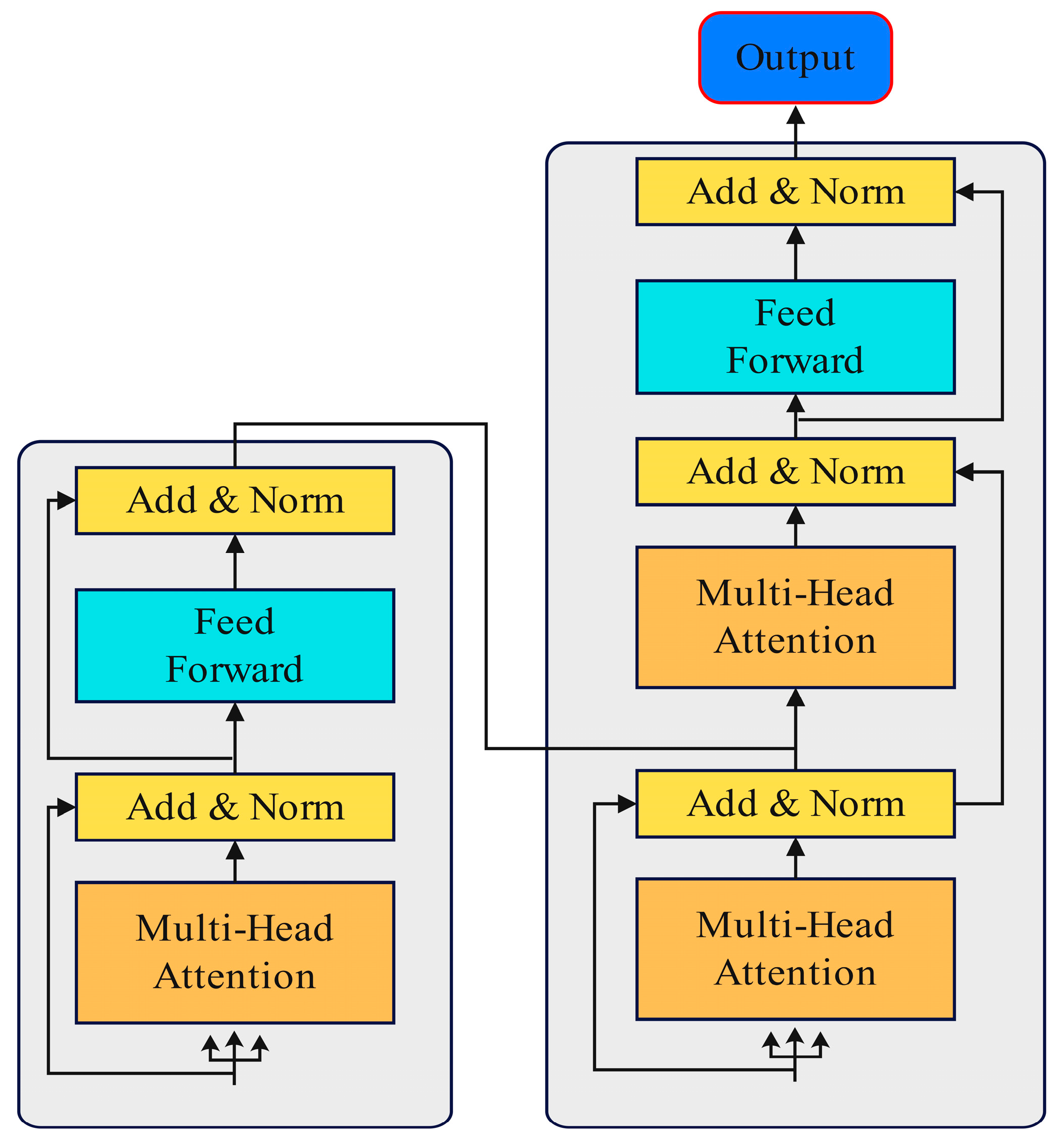
Leveraging its self-attention mechanism, the Transformer overcomes the recursive limitations of traditional recurrent neural networks and captures long-range evolutionary patterns across time steps on a global scale. The model structure is shown in Figure A1.
(1)
Model Formulation
For the input enhanced feature sequence X = { x 1 , x 2 , , x T } R T × D , the Transformer first embeds temporal information via positional encoding, and then maps it through a linear transformation to the query vector Q , the key vector K , and the value vector V :
Q = X W Q ,       K = X W K , V = X W V
where W Q ,   W K ,   W V are learnable weight matrices.
(2)
Self-Attention Mechanism
By calculating the correlation between Q and K , the model can automatically assign weights to different time steps within the sequence. Its output is represented by the weighted sum of the value vectors V :
Attention ( Q , K , V ) = Softmax Q K T d k V
where d k is a scaling factor used to prevent gradient vanishing caused by excessively large dot products. Through parallel computation via multi-head attention, the model can extract global features of wind speed changes and trend components from multiple subspaces.
Figure A1. Transformer model.
Processes 14 02560 g0a1

Appendix A.2. Bidirectional Long Short-Term Memory Network (BiLSTM Model)

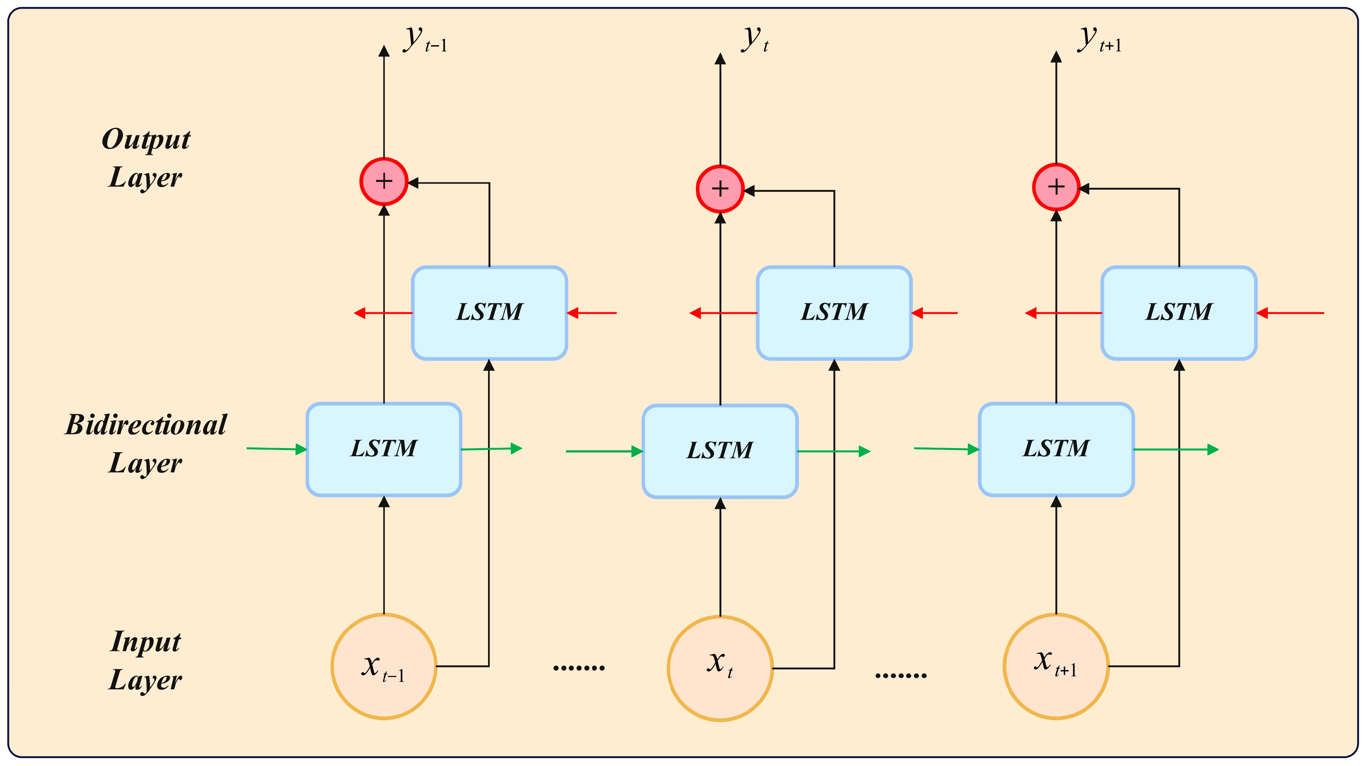
Although the Transformer excels at global modeling, it has limited awareness of the local physical continuity of time-series. The introduction of the Bidirectional Long Short-Term Memory (BiLSTM) network aims to further refine local temporal dynamics features by leveraging its recurrent structure. The model structure is shown in Figure A2.
(1)
Model Structure
The BiLSTM consists of a forward LSTM ( h ) and a backward LSTM ( h ). At each time step t , the model simultaneously considers hidden information from both the past and the future:
h t = LSTM ( x t , h t 1 )
h t = LSTM ( x t , h t + 1 )
The final hidden state is formed by concatenating vectors from both directions: H t = [ h t ;   h t ] .
(2)
Gating Mechanism and Feature Refinement
Each LSTM unit works in concert through the forget gate f t , the input gate i t , and the output gate o t to selectively retain key temporal fluctuation information while suppressing noise:
f t = σ ( W f [ h t 1 , x t ] + b f )
i t = σ ( W i [ h t 1 , x t ] + b i )
Through this bidirectional recurrent mechanism, BiLSTM can effectively capture the “ramp-up” and “ramp-down” trends of wind power output on an extremely short time scale, ensuring that the prediction results align with the continuity of physical motion.
Figure A2. Bi-LSTM model.
Processes 14 02560 g0a2

Appendix B. Evaluation Metrics

To comprehensively quantify the model’s predictive performance, this study selected multiple evaluation metrics from two dimensions: deterministic point prediction and uncertainty interval prediction.

Appendix B.1. Point Forecast Metrics

Point forecasting aims to measure the degree of deviation between the model’s output and actual observed values. This study selected the Mean Absolute Error (MAE), Root Mean Square Error (RMSE), Mean Absolute Percentage Error (MAPE), and Coefficient of Determination ( R 2 ) as evaluation metrics. The definitions of each metric are as follows:
(1)
Mean Absolute Error (MAE)
This is used to reflect the average absolute magnitude of prediction errors; a smaller value indicates higher model accuracy:
MAE = 1 N i = 1 N | y ^ i y i |
(2)
Root Mean Square Error (RMSE)
Because the errors are squared, RMSE is more sensitive to outliers and can effectively highlight significant deviations in the predictions:
RMSE = 1 N i = 1 N ( y ^ i y i ) 2
(3)
Coefficient of Determination ( R 2 )
This is used to evaluate a model’s ability to explain data variability; the closer R 2 is to 1, the better the model’s fit:
R 2 = 1 i = 1 N ( y i y ^ i ) 2 i = 1 N ( y i y _ ) 2
where N is the total number of samples, y i is the actual observed value of the ( i )-th sample, y ^ i is the predicted value, and y _ is the mean of the actual observed values.
(4)
Theil Inequality Coefficient (TIC)
This is used to measure the accuracy of the fit between predicted and actual values; the closer the value is to 0, the more accurate the predictive model:
TIC = 1 n i = 1 n ( y ^ i y i ) 2 1 n i = 1 n y ^ i 2 + 1 n i = 1 n y i 2
where n is the total number of samples, y i is the actual observation for the ( i )-th sample, and y ^ i is the predicted value. This metric eliminates the influence of units and takes values between 0 and 1.
(5)
Consistency Index (IA)
This is used to evaluate the degree of consistency between the model’s predicted values and the observed values; the closer the value is to 1, the better the model’s predictive performance:
IA = 1 i = 1 n ( y ^ i y i ) 2 i = 1 n ( | y ^ i y _ | + | y i y _ | ) 2
where y _ is the mean of the actual observed values. Compared to R 2 , the IA is more sensitive to both additive and multiplicative biases between observed and predicted values.
(6)
Pearson Correlation Coefficient (Pearson R)
This is used to measure the degree of linear correlation between the predicted values and the actual observed values, with a range of [−1, 1]; the closer the absolute value is to 1, the stronger the linear correlation:
R = i = 1 n ( y i y _ ) ( y ^ i y ^ _ ) i = 1 n ( y i y _ ) 2 i = 1 n ( y ^ i y ^ _ ) 2
where y ^ _ is the mean of the predicted values. This metric reflects the model’s ability to capture the trend of wind power fluctuations.
(7)
LogCosh Loss
As a smoothed measure of prediction error, it behaves similarly to the mean squared error (MSE) for small errors and acts as a multiple of the mean absolute error (MAE) for large errors, offering greater robustness:
L ( y , y ^ ) = 1 n i = 1 n log ( cosh ( y ^ i y i ) )
Compared to traditional MSE, this metric reduces the interference of outliers on model training, making the prediction curve more robust at points of severe fluctuations.
(8)
N M A E and N R M S E
To enable normalized performance comparison across different wind farm capacities, Normalized Mean Absolute Error ( N M A E ) and Normalized Root Mean Square Error ( N R M S E ) are defined as follows:
N M A E = M A E P c a p × 100 % = 1 N t = 1 N P t P ^ t P c a p × 100 %
N R M S E = R M S E P c a p × 100 % = 1 N t = 1 N P t P ^ t 2 P c a p × 100 %
where P t and P ^ t are the actual and predicted active power at time t , N is the number of test samples, and P c a p is the total nominal installed capacity ( 200   MW for Dataset A and 100   MW for Dataset B). These normalized metrics eliminate capacity-scale bias and measure relative prediction errors against facility capacity.

Appendix B.2. Interval Prediction Metrics

The core of evaluating interval prediction (with a confidence level of 1 α ) lies in balancing the reliability (Coverage) and sharpness (Sharpness) of the confidence interval. This study employs the Probability of Interval Coverage (PICP), the Probability of Interval Normalized Average Width (PINAW), and the Coverage Error (CWC).
(1)
Probability of Inclusion in the Prediction Interval (PICP)
PICP measures the frequency with which actual observations fall within the prediction interval, reflecting the reliability of the prediction. Ideally, PICP should be greater than or equal to the preset confidence level (e.g., 95%):
PICP = 1 N i = 1 N c i ,     c i = 1 , y i [ L i , U i ] 0 , y i [ L i , U i ]
where L i and U i represent the lower and upper bounds of the prediction interval, respectively.
(2)
Predicted Interval Normalized Average Width (PINAW)
Given that coverage requirements are met, the narrower the prediction interval, the greater the certainty of the prediction. PINAW is normalized to facilitate comparisons across different datasets:
PINAW = 1 N R i = 1 N ( U i L i )
where R is the target variation range of the observed value (the difference between the maximum and minimum values).
(3)
Comprehensive Coverage Metric (CWC)
CWC combines reliability and sharpness to evaluate the overall quality of an interval through a penalty mechanism. When PICP falls below the confidence level μ = 1 α , CWC is subject to an exponential penalty:
CWC = PINAW ( 1 + γ e η ( PICP μ ) )
where γ is an indicator variable controlling the penalty strength: when PICP μ , γ = 0 ; when PICP < μ , γ = 1 . η is a hyper parameter used to amplify the penalty resulting from insufficient coverage.

References

  1. IRENA. World Energy Transitions Outlook 2023: 1.5 °C Pathway; International Renewable Energy Agency: Abu Dhabi, United Arab Emirates, 2023. [Google Scholar]
  2. Zou, J.; Wang, Z.; Zhu, Z.; Tan, Z. Explainable and physics-constrained PV power prediction via a hybrid framework integrating secondary decomposition and improved Transformer-LSTM. Energy 2026, 347, 140314. [Google Scholar] [CrossRef]
  3. Wang, K.; Wang, L.; Meng, Q.; Yang, C.; Lin, Y.; Zhu, J.; Zhao, Z.; Zhou, C.; Zheng, C.; Gao, X. Accurate photovoltaic power prediction via temperature correction with physics-informed neural networks. Energy 2025, 328, 136546. [Google Scholar] [CrossRef]
  4. Wang, Z.; Ma, C.; Tan, Z.; Wu, T. Low-carbon development pathways for the water-energy-food-carbon nexus in the Yangtze river economic Belt: Insights from coupling coordination and obstacle degree analysis. J. Clean. Prod. 2025, 523, 146399. [Google Scholar] [CrossRef]
  5. Foley, A.; Gallachóir, B.Ó.; Hur, J.; Baldick, R.; McKeogh, A. A strategic review of electricity systems models. Energy 2023, 263, 126132. [Google Scholar]
  6. Zhu, Z.; Wang, Z.; Wu, H.; Liu, C.; Tan, Z.; Ren, T.; Liu, Q. Dynamic scheduling of cascaded reservoirs: A full-cycle framework for integrating the economic–social–ecological nexus for sustainable management. J. Hydrol. 2026, 672, 135328. [Google Scholar] [CrossRef]
  7. Szostek, K.; Mazur, D.; Drałus, G.; Kusznier, J. Analysis of the Effectiveness of ARIMA, SARIMA, and SVR Models in Time Series Forecasting: A Case Study of Wind Farm Energy Production. Energies 2024, 17, 4803. [Google Scholar] [CrossRef]
  8. Syamsuddin, A.; Adhi, A.C.; Widodo, A.; Prahasto, T.; Kusumawardhani, A. Photovoltaic system power output forecasting using vector auto-regression (VAR). In Proceedings of the 2024 6th International Conference on Power Engineering and Renewable Energy (ICPERE), Bandung, Indonesia, 5–6 November 2024. [Google Scholar]
  9. Liu, P.; Li, M.; Han, C.; Meng, L.; Shao, Z. From input to output: Unraveling the spatio-temporal pattern and driving factors of the coupling coordination between wind power efficiency and installed capacity in China. Renew. Energy 2025, 396, 126320. [Google Scholar] [CrossRef]
  10. Guliyev, H. Nexus between renewable energy and economic growth in G7 countries: New insight from nonlinear time series and panel cointegration analysis. J. Clean. Prod. 2023, 424, 138853. [Google Scholar] [CrossRef]
  11. Wen, B.; Wei, S.; Wei, K.; Yang, W.; Peng, Z.; Chu, F. Power fluctuation and power loss of wind turbines due to wind shear and tower shadow. Front. Mech. Eng. 2017, 12, 321–332. [Google Scholar] [CrossRef]
  12. Benali, L.; Notton, G.; Fouilloy, A.; Voyant, C.; Dizene, R. Solar radiation forecasting using artificial neural network and random forest methods: Application to normal beam, horizontal diffuse and global components. Renew. Energy 2023, 209, 18–34. [Google Scholar]
  13. Aksoy, N.; Genc, I. Predictive models development using gradient boosting based methods for solar power plants. J. Comput. Sci. 2023, 67, 101958. [Google Scholar] [CrossRef]
  14. Chaudhari, T.; Joshi, A.; Bharti, D.; Chavan, P.; Deshmukh, M.K.; Bhalgat, P. A Comparative Study of Ensemble Learning Models for Accurate Solar Irradiance Forecasting. In Proceedings of the 2024 8th International Conference on Computational System and Information Technology for Sustainable Solutions (CSITSS), Bengaluru, India, 7–9 November 2024. [Google Scholar]
  15. Wei, Z.; Zhao, D. Efficient Short-Term Wind Power Prediction Using a Novel Hybrid Machine Learning Model: LOFVT-OVMD-INGO-LSSVR. Energies 2025, 18, 1849. [Google Scholar] [CrossRef]
  16. Wood, M.; Ogliari, E.; Nespoli, A.; Simpkins, T.; Leva, S. Day Ahead Electric Load Forecast: A Comprehensive LSTM-EMD Methodology and Several Diverse Case Studies. Forecasting 2023, 5, 297–314. [Google Scholar] [CrossRef]
  17. Yang, Y.; Wang, J.; Chen, B.; Yan, H. Pseudo-Twin Neural Network of Full Multi-Layer Perceptron for Ultra-Short-Term Wind Power Forecasting. Energies 2025, 14, 887. [Google Scholar] [CrossRef]
  18. Cheng, L.; Chengbo, Y.; Cheng, H.; Chunlin, Z.; Wei, Z.; Jia, C. Ultra-short-term Wind Power Prediction Based on Dual-stage Attention Mechanism CNN-BiLSTM and LightGBM Error Correction. J. Electr. Eng. 2024, 19, 137–145. [Google Scholar]
  19. Agga, A.; Abbou, A.; Labbadi, M.; El Houm, Y. Short-term self consumption PV plant power production forecasts based on hybrid CNN-LSTM, ConvLSTM models. Renew. Energy 2021, 177, 101–112. [Google Scholar] [CrossRef]
  20. Bashir, T.; Wang, H.; Tahir, M.; Zhang, Y. Wind and solar power forecasting based on hybrid CNN-ABiLSTM, CNN-transformer-MLP models. Renew. Energy 2025, 239, 122055. [Google Scholar] [CrossRef]
  21. Zhang, Z.; Ye, Y.; Qin, H.; Liu, Y. Hybrid CNN-LSTM model with VMD decomposition for short-term wind power forecasting. Energy 2023, 276, 127582. [Google Scholar] [CrossRef]
  22. Jiang, C.; Zhu, Q. Evaluating the most significant input parameters for forecasting global solar radiation of different sequences based on Informer. Appl. Energy 2023, 348, 121544. [Google Scholar] [CrossRef]
  23. Qu, K.; Xue, S.; Zheng, X.; Yan, D.; Cao, H. Learning dynamic inter-farm dependencies for wind power forecasting via adaptive sparse graph attention network. Renew. Energy 2024, 225, 124969. [Google Scholar] [CrossRef]
  24. Zhao, Y.; Liao, H.; Pan, S.; Zhao, Y. Interpretable multi-graph convolution network integrating spatio-temporal attention and dynamic combination for wind power forecasting. Expert Syst. Appl. 2024, 255, 124766. [Google Scholar] [CrossRef]
  25. Pan, Y.; Wang, Z.; Tan, Z.; Zhu, Z. Interpretable photovoltaic power modeling via kolmogorov-arnold network and timeGAN hybrid architecture with regime-aware data augmentation. Sol. Energy 2025, 302, 114022. [Google Scholar] [CrossRef]
  26. Benti, N.E.; Chaka, M.D.; Semie, A.G. Forecasting Renewable Energy Generation with Machine Learning and Deep Learning: Current Advances and Future Prospects. Sustainability 2023, 15, 7086. [Google Scholar] [CrossRef]
  27. Li, D.; Pan, Q.; Lei, S.; Hu, Z.; Li, Y.; Yao, B. Nonparametric probabilistic forecasting of wind power based on adaptive copula and quadratic spline quantile function. Sustain. Energy Grids Netw. 2026, 47, 102346. [Google Scholar] [CrossRef]
  28. Li, K.; Duan, P.; Xue, Q.; Cheng, Y.; Hua, J.; Chen, J.; Guo, P. Enhancing reliability assessment in distributed generation networks: Incorporating dynamic correlation of wind-solar power output uncertainty. Sustain. Energy Grids Netw. 2024, 39, 101512. [Google Scholar] [CrossRef]
  29. Zhu, Z.; Wu, H.; Wang, Z.; Zhang, X.; Kong, J.; Liu, C.; Tan, Z.; Liu, Q. Physics-AI synergized optimization-learning-simulation framework for robust cascade reservoir scheduling under future hydrological uncertainty. Water Resour. Res. 2026, 62, e2025WR042149. [Google Scholar] [CrossRef]
  30. Ding, C.; Wang, Z.; Tan, Z.; Zhang, X. Multi-source heterogeneous data-driven interpretable model based on transformer and kolmogorov-arnold networks for streamflow prediction. Expert Syst. Appl. 2026, 328, 132862. [Google Scholar] [CrossRef]
  31. He, Y.; Wang, Z.; Cheng, H.; Ding, W. Multi-scale feature fusion and uncertainty quantification in streamflow prediction: A temporal convolutional network approach with hybrid denoising. Environ. Model. Softw. 2026, 198, 106879. [Google Scholar] [CrossRef]
  32. Elizondo, M.A.; Lu, S.; Zhou, N.; Samaan, N. Model reduction, validation, and calibration of wind power plants for dynamic studies. In Proceedings of the 2011 IEEE PES General Meeting, Detroit, MI, USA, 24–28 July 2011. [Google Scholar]
  33. Liu, Z.; Wang, Y.; Vaidya, S.; Ruehle, F.; Halverson, J.; Soljačić, M.; Hou, T.Y.; Tegmark, M. KAN: Kolmogorov-Arnold Networks. arXiv 2024, arXiv:2404.14756. [Google Scholar]
  34. Nie, Y.; Nguyen, N.H.; Sinthong, P.; Kalagnanam, J. A time series is worth 64 words: Long-term forecasting with transformers. In International Conference on Learning Representations (ICLR); ICLR: Appleton WI, USA, 2023. [Google Scholar]
  35. Lim, B.; Arık, S.Ö.; Loeff, N.; Pfister, T. Temporal fusion transformers for interpretable multi-horizon time series forecasting. Int. J. Forecast. 2021, 37, 1748–1764. [Google Scholar] [CrossRef]
Figure 1. Flowchart of the FW-BTP hybrid prediction model proposed in this study.
Processes 14 02560 g001
Figure 2. Multi-model Comparison Line Chart.
Processes 14 02560 g002
Figure 3. Multi-model Comparison Scatter Plot.
Processes 14 02560 g003
Figure 4. Comparison of the performance of different prediction models after multiple runs.
Processes 14 02560 g004
Figure 5. Performance comparison chart of modules in the ablation experiment. ((a) Radar plot of ablation experiments; (b) dual-Y-axis plot of different metrics; (c) compass plot of ablation experiments).
Processes 14 02560 g005
Figure 6. Comparison of probabilistic prediction performance.
Processes 14 02560 g006
Figure 7. Comparison of model prediction performance for Dataset B.
Processes 14 02560 g007
Figure 8. Model feasibility analysis.
Processes 14 02560 g008
Figure 9. Comparison of the latest model performance: (1) latest model wind power forecasting comparison map, (2) Taylor diagram comparison, (3) distribution analysis: MAE, (4) distribution analysis: RMSE.
Processes 14 02560 g009
Table 1. Structural specifications and hyperparameters of the FW-BTP framework.
Component/ParameterDetailed Specification/Value
Input Look-back Window (T)24 steps (6 h at 15 min resolution)
Prediction Horizon1 step (t + 1, single-step rolling forecast)
BiLSTM Backbone2 hidden layers, h d i m = 64 (bidirectional output dimension: 128)
Transformer Encoder2 encoder layers, n h e a d = 4 attention heads, d m o d e l = 64 ,   d f f = 128 , Dropout = 0.10
Optimization SetupAdamW ( η = 1 × 1 0 3 , weight decay = 1 × 1 0 4 ), CosineAnnealingLR ( T m a x = 50 )
Training SettingsBatch size = 64, maximum epochs = 100, early stopping patience = 15
Component/ParameterDetailed Specification/Value
Table 2. Comparison of prediction performance among different models.
ModelR2MAERMSENMAE (%)NRMSE (%)
MLP0.9552 ± 0.00139.5590 ± 0.842315.3713 ± 0.2292 4.7795 ± 0.4212 7.6857 ± 0.1146
RNN0.9590 ± 0.00079.0000 ± 0.566814.6703 ± 0.1178 4.5000 ± 0.2834 7.3352 ± 0.0589
LSTM0.9606 ± 0.00128.1625 ± 0.198414.5103 ± 0.2214 4.0813 ± 0.0992 7.2552 ± 0.1107
GRU0.9599 ± 0.00038.6048 ± 0.239014.4445 ± 0.0444 4.3024 ± 0.1195 7.2223 ± 0.0222
Bi-LSTM0.9575 ± 0.00088.7502 ± 0.188614.8089 ± 0.1394 4.3751 ± 0.0943 7.4045 ± 0.0697
CNN-LSTM0.9602 ± 0.00118.3744 ± 0.321814.5204 ± 0.1886 4.1872 ± 0.1609 7.2602 ± 0.0943
TCN0.9337 ± 0.001611.1228 ± 0.511118.5241 ± 0.2164 4.1872 ± 0.1609 9.2621 ± 0.1082
Transformer0.5742 ± 0.104253.3386 ± 4.410461.5989 ± 5.5986 4.1872 ± 0.1609 30.7995 ± 2.7993
FW-BTP0.9967 ± 0.00026.1166 ± 0.269011.1972 ± 0.4862 4.1872 ± 0.1609 5.5986 ± 0.2431
Table 3. Performance comparison table of ablation experiments.
ModelMAERMSER2TICIAPearson RLogCosh
Proposed6.116611.19720.99670.04620.99590.99215.1167
without WGM10.181415.00330.95640.07730.98820.98079.5664
without FCM7.926913.71150.96360.07000.99060.98337.2955
without PGL6.692611.28040.97540.05590.99390.98826.0695
Table 4. Probabilistic forecasting performance metrics.
ModelR2MAEPICP (95%)PINAWCWC
MLP0.95149.40120.93380.33891.1025
RNN0.95968.56330.95600.26220.2622
GRU0.95579.21500.91030.22931.8957
LSTM0.95968.32990.94000.21550.5701
BiLSTM0.95968.33010.95260.24930.2493
CNN-LSTM0.96108.47710.96570.25000.2500
TCN0.923611.93070.94120.35240.9001
Transformer0.94199.82630.92580.22820.9950
FW-BTP0.97805.46320.94690.12210.2648
Table 5. Analysis metrics for the dataset.
ModelR2MAERMSE
MLP0.97661.72892.8682
RNN0.98331.31732.4210
LSTM0.98381.26832.3904
GRU0.98171.42332.5385
BiLSTM0.98231.43112.4974
CNN-LSTM0.98191.37392.5208
TCN0.98291.35782.4515
Transformer0.89863.94445.9706
FW-BTP0.99061.09171.8228
Table 6. Comparison of the latest model performance.
ModelR2MAERMSE
KAN [33]0.95029.666616.0398
Patch-Informer [34]0.95549.092215.1729
TFT-Light [35]0.95958.761914.4561
FW-BTP0.99676.116611.1972
Disclaimer/Publisher’s Note: The statements, opinions and data contained in all publications are solely those of the individual author(s) and contributor(s) and not of MDPI and/or the editor(s). MDPI and/or the editor(s) disclaim responsibility for any injury to people or property resulting from any ideas, methods, instructions or products referred to in the content.